Singapore Management University
Institutional Knowledge at Singapore Management University
Research Collection School Of Economics
School of Economics
2-2015
Shrinkage estimation of dynamic panel data models
with interactive fixed effects
Xun LU
Hong Kong University of Science and Technology
Liangjun SU
Singapore Management University, [email protected]
Follow this and additional works at:
https://ink.library.smu.edu.sg/soe_research
Part of the
Econometrics Commons
This Working Paper is brought to you for free and open access by the School of Economics at Institutional Knowledge at Singapore Management University. It has been accepted for inclusion in Research Collection School Of Economics by an authorized administrator of Institutional Knowledge at Singapore Management University. For more information, please [email protected].
Citation
LU, Xun and SU, Liangjun. Shrinkage estimation of dynamic panel data models with interactive fixed effects. (2015). 1-94. Research Collection School Of Economics.
ANY OPINIONS EXPRESSED ARE THOSE OF THE AUTHOR(S) AND NOT NECESSARILY THOSE OF
Shrinkage Estimation of Dynamic Panel Data
Models with Interactive Fixed Effects
Xun Lu and Liangjun Su
February 2015
Shrinkage Estimation of Dynamic Panel Data Models with
Interactive Fixed E
ff
ects
∗
Xun Lu
and Liangjun Su
Department of Economics, HKUST
School of Economics, Singapore Management University
February 2, 2015
Abstract
We consider the problem of determining the number of factors and selecting the proper regressors in linear dynamic panel data models with interactivefixed effects. Based on the preliminary estimates of the slope parameters and factorsa laBai and Ng (2009) and Moon and Weidner (2014a), we propose a method for simultaneous selection of regressors and factors and estimation through the method of adaptive group Lasso (least absolute shrinkage and selection operator). We show that with probability approaching one, our method can correctly select all relevant regressors and factors and shrink the coefficients of irrelevant regressors and redundant factors to zero. Further, we demonstrate that our shrinkage estimators of the nonzero slope parameters exhibit some oracle property. We conduct Monte Carlo simulations to demonstrate the superbfinite-sample performance of the proposed method. We apply our method to study the determinants of economic growth andfind that in addition to three common unobserved factors selected by our method, government consumption share has negative effects, whereas investment share and lagged economic growth have positive effects on economic growth.
JEL Classification: C13, C23, C51
Key Words:Adaptive Lasso; Dynamic panel; Factor selection; Group Lasso; Interactivefixed effects; Oracle property; Selection consistency
∗The authors gratefully thank the Co-editor Cheng Hsiao, the Associate Editor, and three anonymous referees for their
many constructive comments on the previous version of the paper. They express their sincere appreciation to Jushan Bai, Songnian Chen, Xiaohong Chen, Han Hong, Lung-Fei Lee, Qi Li, Hyungsik Roger Moon, Peter C. B. Phillips, and Peng Wang for discussions on the subject matter and valuable comments on the paper. They also thank the conference and seminar participants at the 3rd Shanghai Econometrics Workshop, Tsinghua International Conference in Econometrics, 2013, and Peking University for their valuable comments. Su gratefully acknowledges the Singapore Ministry of Education for Academic Research Fund under grant number MOE2012-T2-2-021. Address Correspondence to: Liangjun Su, School of Economics, Singapore Management University, 90 Stamford Road, Singapore 178903; E-mail: [email protected], Phone: +65 6828 0386.
1
Introduction
We consider a panel data model with interactivefixed effects as proposed and studied in Pesaran (2006), Bai (2009), Moon and Weidner (2014a, 2014b), Pesaran and Tosetti (2011), Greenaway-McGrevy et al. (2012), Su and Jin (2012), Su et al. (2015), among others. This model has been widely applied in empirical research, as it allows more flexible modeling of heterogeneity than traditional fixed effects models and provides an effective way to model cross section dependence that is widely present in macro and financial data. To use this model, we need to determine the number of factors in the multi-factor error component and select the proper regressors to be included in the model. This paper provides a novel automated estimation method that combines both estimation of parameters of interest and selection of the number of factors and regressors.
Specifically, we consider the following interactivefixed-effects panel data model
=00+000+ = 1 = 1 (1.1) where is a 0×1vector of regressors,0 is the corresponding vector of slope coefficients, 0 is an
0×1vector of unknown factor loadings,0 is an 0×1vector of unknown common factors, and is the idiosyncratic error term. Here the factor structure 000 is referred to as interactive fixed effects in Bai (2009) and Moon and Weidner (2014a, 2014b) as one allows both 0 and 0
to be correlated with elements of and000+ is called the multi-factor error structure in Pesaran (2006). We are interested in estimating 0 0 and 0 It has been argued that the factor structure can capture more
flexible heterogeneity across individuals and over time than the traditionalfixed-effects model. The latter takes the form = 00+0 +0 + and can be thought of as a special case of the interactive
fixed-effects panel data model by letting0= (1 0)0 and0 = (01)0where 0 and
0
are individual-specific and time-specificfixed effects, respectively. When is absent in (1.1), the model becomes the pure factor model studied in Bai and Ng (2002) and Bai (2003), among others.
Given the correct number0of factors and the proper regressorsseveral estimation methods have been proposed in the literature. For example, Pesaran (2006) proposes common correlated effects (CCE) estimators; Bai (2009) and Moon and Weidner (2014a, 2014b) provide estimators based on Gaussian quasi-maximum likelihood estimation (QMLE) and the principal component analysis (PCA). To apply the latter methods, we must first determine the number of factors and appropriate regressors to be included in the model. Nevertheless, in practice, we do not have a priori knowledge about the true number of factors in almost all cases. Also there may be a large number of potential regressors, some of which may be irrelevant. Thus it is desirable to use a parsimonious model by choosing a subset of regressors. The common procedure is to perform some model selection in thefirst step and then conduct estimation based on the selected regressors and the chosen number of factors. To select regressors, a wide range of methods can be adopted. For example, one can apply the Bayesian information criterion (BIC) or some cross-validation methods. To determine the number of factors, one can apply the information criteria proposed in Bai and Ng (2002) or the testing procedure introduced in Onatski (2009, 2010), Kapetanios (2010), or Ahn and Horenstein (2013). Bai and Ng (2006, 2007) provide some empirical examples of the determination of number of factors in economic applications. Hallin and Li´ska (2007) study the determination of the number of factors in general dynamic factor models.
In this paper, we explore a different approach. We use shrinkage techniques to combine the estimation with the selection of the number of factors and regressors in a single step. Following Bai (2009) or Moon and Weidner (2014a, 2014b), we can set a maximum number of factors (say) and obtain the preliminary estimates of the slope parameters and factors. Then we consider a penalized least squares (PLS) regression of on and the estimated factors via the adaptive (group) Lasso. We include two penalty terms in the PLS, one for the selection of regressors in via adaptive Lasso and the other for the selection of the exact number of factors via adaptive group Lasso. Despite the use of estimated factors that have slow convergence rates, we show that our new method can consistently determine the number of factors,consistently select all relevant regressors, and shrink the estimates of the coefficients of irrelevant regressors and redundant factors to zerowith probability approaching 1 (w.p.a.1). We also demonstrate the oracle property of our method. That is, our estimator of the non-zero regression coefficients is asymptotically equivalent to the least squares estimator based on the factor-augmented regression where both the true number of factors and the set of relevant regressors areknown. The bias-corrected version of our shrinkage estimator of the non-zero regression coefficients is asymptotically equivalent to Moon and Weidner’s (2014b) bias-corrected QML estimator in the case where all regressors arerelevant (i.e., there is no selection of regressors). In the presence ofirrelevantregressors, the variance-covariance matrix for our shrinkage estimator of the non-zero coefficients is smaller than that of Moon and Weidner’s QML estimator. In addition, we emphasize that even though Moon and Weidner (2014a) show that the limiting distribution of the QML estimator is independent of the number of factors used in the estimation as long as the number of factors does not fall below the true number of factors, wefind that infinite samples the inclusion of redundant factors can result in significant loss of efficiency (see Section 4.3 for detail). For this reason, it is very important to include the correct number of factors in the model especially when the cross section or time dimension is not very large. Our shrinkage method effectively selects allrelevant
regressors and factor estimates and get rid of irrelevant regressors or redundant factor estimates. There is a large statistics literature on the shrinkage type of estimation methods. See, for example, Tibshirani (1996) for the origin of Lasso, Knight and Fu (2000) for the first systematic study of the asymptotic properties of Lasso-type estimators, and Fan and Li (2001) for SCAD (smoothly clipped absolute deviation) estimators. Zou (2006) establishes the oracle property of adaptive Lasso; Yuan and Lin (2006) propose the method of group Lasso; Wang and Leng (2008) and Wei and Huang (2010) study the properties of adaptive group Lasso; Huang et al. (2008) study Bridge estimators in sparse high dimensional regression models. Recently there have been an increasing number of applications of the shrinkage techniques in the econometrics literature. For example, Caner (2009) and Fan and Liao (2014) consider covariate selection in GMM estimation. Belloni et al. (2013) and García (2011) consider selection of instruments in the GMM framework. Liao (2013) provides a shrinkage GMM method for moment selection and Cheng and Liao (2015) consider the selection of valid and relevant moments via penalized GMM. Liao and Phillips (2015) apply adaptive shrinkage techniques to cointegrated systems. Kock (2013) considers Bridge estimators of static linear panel data models with random or fixed effects. Caner and Knight (2013) apply Bridge estimators to differentiate a unit root from a stationary alternative. Caner and Han (2014) propose a Bridge estimator for pure factor models and shows the selection consistency. Cheng et al. (2014) provide an adaptive group Lasso estimator for pure factor structures with possible
structural breaks. This paper adds to the literature by applying the shrinkage idea to panel data models with factor structures and considering generated regressors.
The method proposed in this paper has a wide range of applications. For example, it can be used to estimate a structural panel model that allows a more flexible form of heterogeneity. A specific example is to study cross-country economic growth. Let be the economic growth for country in period and be a large number of potential observable causes of economic growth, such as physical capital investment, consumption, population growth, government consumption, and lagged economic growth, among others. Economic growth may also be caused by many unobservable common factors 0
. It is of great interest to know which observable causes are important to determine economic growth and the number of common unobserved factors that affect all countries’ economic growth. Our new method is directly applicable to this important economic question. Another example of application is to forecast asset returns, as factor models are often used to model asset returns. Specifically, let be the excess returns on asset in period and be observable factors such as Fama-French factors (small market capitalization and book-to-market ratio), divided yields, dividend payout ratio and consumption gap, among others. The asset returns may also be affected by an unknown number of common unobserved factors. Our method automatically selects the important observable factors and unobservable common factors. Thus it provides a powerful tool to predict future asset returns.
The paper is organized as follows. Section 2 introduces our adaptive group Lasso estimators. Section 3 analyzes their asymptotic properties. In Section 4, we report the Monte Carlo simulation results for our method and compare it with the methods of Bai and Ng (2002), Onatski (2009, 2010), and Ahn and Horenstein (2013). In Section 5, we apply our method to study the determinants of economic growth in the framework of dynamic panel data models with interactivefixed effects, andfind that in addition to three common unobserved factors selected by our method, government consumption share has negative effects, whereas investment share and lagged economic growth have positive effects on economic growth. Final remarks are contained in Section 6. The proofs of all theorems are delegated to Appendix B. Additional materials are provided in the online supplementary Appendices C-F.
NOTATION. For an ×real matrix we denote its transpose as0 its Frobenius norm askk
(≡[tr(0)]12) its spectral norm askk
sp (≡
p
1(0)) and its Moore-Penrose generalized inverse
as +where ≡means “is defined as” and
(·)denotes the th largest eigenvalue of a real symmetric matrix by counting eigenvalues of multiplicity multiple times. Note that the two norms are equal when
is a vector. We will frequently use the submultiplicative property of these norms and the fact that
kksp≤kk≤kksprank()12We also usemax()andmin()to denote the largest and smallest eigenvalues of a symmetric matrix, respectively. We use 0to denote that is positive definite. Let≡(0)+0 and≡− wheredenotes an×identity matrix. The operator
→denotes convergence in probability,→ convergence in distribution, and plim probability limit. We use
2
Penalized Estimation of Panel Data Models with Interactive
Fixed E
ff
ects
In this section, we consider penalized least squares (PLS) estimation of panel data models with interactive
fixed effects where the number of unobservable factors is unknown and some observable regressors may be irrelevant.
2.1
Panel Data Models with Interactive Fixed E
ff
ects
We assume that the true model (1.1) is unknown, in particular, 0 and0 are unknown. With a little
bit abuse of notation, we consider their empirical model
=00+000+ = 1 = 1 (2.1) whereis a×1vector of regressors that may contain lagged dependent variables,0≡
¡
01 0¢0
is a×1vector of unknown slope coefficients,0and0 are×1vectors of factors and factor loadings, respectively, andis the idiosyncratic error term. Here©0
ª
and©0
ª
may be correlated with{} We consider estimation and inference on0 when the true number of factors0 (≤)is unknown and
some variables inmay be irrelevant, i.e., 0≤In the sequel, we allow both and0to pass to
infinity as( )→ ∞but assume that isfixed to facilitate the asymptotic analysis. To proceed, letdenote theth element of for= 1 Define
≡ (1 )0 ≡(1 )0 ≡(1 )0
0 ≡ ¡10 0¢0 0≡¡01 0¢0 ·≡(1 )0 Y ≡ (1 )0 X ≡(1· ·)0 andε≡(1 )0
ApparentlyYX andεare all× matrices. Then we can write the model (2.1) in matrix form
Y=
X
=1
0X+000+ε (2.2)
Without loss of generality (Wlog), we assume that only thefirst0 elements of have nonzero slope coefficients, and write= (0(1) 0(2))0where(1)and(2)are0×1and(−0)×1vectors,
respectively, and the true coefficients of(1) are nonzero while those of (2) are zero. Accordingly,
we decompose0 as0= ((1)00 0(2)0 )0= (00 (1)00)0
2.2
QMLE of
¡
0
0
0¢
Givenand all regressors, following Bai (2009) and Moon and Weidner (2014a, 2014b), we consider the Gaussian QMLE(˜˜˜)of¡0 0 0¢which is given by
³ ˜ ˜ ˜´= arg min () L 0 ( ) (2.3)
where L0 ( )≡ 1 tr ⎡ ⎣ Ã Y− X =1 X−0 !0Ã Y− X =1 X−0 !⎤ ⎦ (2.4)
≡(1 )0 is a×1vector,≡(1 )0 is a×matrix, and≡(1 )0 is an× matrix. One canfirst obtain the profile-likelihood estimate˜and then the estimate (˜ ˜) via the PCA method under the identification restrictions: 0 = and 0is a diagonal matrix. Namely, (˜ ˜)
solves " 1 X =1 ³ −˜ ´ ³ −˜ ´0# ˜ = ˜ and˜=−1 Ã Y− X =1 ˜ X ! ˜ (2.5)
where is a diagonal matrix consisting of thelargest eigenvalues of the above matrix in the square bracket, arranged in descending order. Moon and Weidner (2014a) show that as long as ≥0 the
limiting distribution of the QMLE for is independent of , the number of unobserved factors used in the estimation. Throughout the paper, we assume that≥0 and use˜
= (˜1 ˜)0 to denote the
bias-corrected version of ˜ based on the formula in Moon and Weidner (2014b) or our supplementary Appendix F. After obtaining˜we obtain thefinal estimate (˜ ˜) via (2.5) with˜ replaced by˜
2.3
Penalized Least Squares Estimation of
¡
0
∗¢
We first present our PLS estimators and then provide some motivations for them. Our PLS estimator
(ˆˆ)are obtained as follows.
• Estimate model (2.1) with factors and all regressors and obtain (˜˜) and˜ as discussed in Section 2.2.
• LetYˆ =Y−P=1˜
Xˆ= ( )−1Yˆ0Yˆ ˜ andΣˆˆ =−1ˆ0 ˆ Compute theeigenvalues of
ˆ
Σˆ arranged in descending order and denote them as1 .
• Minimize the following PLS criterion function
( ) =L ( ) +1 X =1 1 ¯ ¯ ¯˜¯¯¯1 | |+√2 X =1 1 2 k ·k (2.6)
where L ( ) = L0 ( ˆ) · denotes the th column of = = (1 2 ) is a vector of tuning parameters, and 1 2 0 are usually taken as either 1 or 2. Let (ˆˆ) =
(ˆ()ˆ())denote the solution to the above minimization problem.
Note that (2.6) contains two penalty terms, 1 for the regression coefficients ’s and 2 for the loading vectors ·’s. Noting that −12k·k =(1) under our Assumption A.1(iii) in Section 3.1 which apparently rules out the case of weak factors studied by Onatski (2012), we divide the second penalty term 2 by √. Note that the objective function in (2.6) is convex in ( ) so that the global minimizer of can be found easily for any given tuning parameterWe frequently suppress the dependence of(ˆˆ)onas long as no confusion arises. Below we will propose a data-driven method to chooseAlso, note that we have used estimated factorsˆ in (2.6).
As a referee points out, the idea to use group Lasso for selection of the number of factors has been around for some time. For example, Hirose and Konishi (2012) derive a model selection criterion for selecting factors in a pure factor model but they do not provide asymptotic analysis. In contrast, we consider both variable and factor selections in dynamic panel data models and offer systematic asymptotic analysis.
Our procedure is motivated by the literature on adaptive group Lasso (see, Yuan and Lin (2006), Zou (2006), Huang et al. (2008)). Now we provide some details. is usually different from 0 and
one cannot expect ˜ to be a consistent estimator of 0 or a rotational version of 0. Define =
=
¡
−1000¢(−100˜)We can follow Bai and Ng (2002) and show that under certain regularity
conditions, 1 ° ° °ˆ−0°° °2= ¡ −2¢and°°°ˆ−00 ° ° °2= ¡
− 2¢for eachwhereˆ0
denotes the
th row of ˆ and = min( √
√)In addition, we show in Appendix A that = converges in probability to a sparse matrix
0= [(1)0 00×(−0)]
where 0
(1) is an 0×0 full rank matrix and 0× denotes an × matrix of zeros. As a result,
∗ =+0
also exhibits a sparse structure asymptotically, i.e., the last(−0)elements of∗ converge in probability to zero. Using the above definitions of and ∗we can rewrite (2.1) as1
=00+00+000+=00+∗000+ (2.7) The sparse nature of ∗ (and 0) suggests that we can apply an adaptive group Lasso procedure as introduced above. Further, we show in Appendix A that1 0 converge in probability to somefinite positive numbers whereas0+1 converge to zero at
√
-rate. This means thatΣˆˆ provides the
information on the sparsity nature of∗This motivates us to use 12
as a weight in the second penalty
term in (2.6).
3
Asymptotic Properties
In this section we study the asymptotic properties of the proposed adaptive group Lasso estimator(ˆˆ)
3.1
Estimation Consistency
Let¯ = 1 P=10and = 1 P=1˜00˜where˜≡−1 P =1 00 ¡ −1000¢−10 Let denote a generic finite positive constant that may vary across lines. We make the following assumptions.
Assumption A.1(i)p °°°˜−0°°°=(1)and √ ¯¯¯˜−0¯¯¯=(1)for each= 1 (ii)°°0 ° °8 ≤ and−1000−→ Σ
00for some0×0 matrixΣ0 as → ∞ (iii)°°0°°8≤ and−1000
−→Σ0 0for some 0×0 matrixΣ0 as → ∞ (iv) For= 1 ( )−1kXk2≤
1Noting that the
0×matrixis right invertible, by Proposition 6.1.5 in Bernstein (2005, p.225) we have+=
0(0)−1which further implies that+=
(v)kεksp=(max( √
√))
(vi) For= 1 ( )−1[tr(Xε0)]2≤ (vii)( )−1°°00ε0°°2≤
(viii) There are two nonstochastic × matrices¯0 and 0 such that
°
°¯ −¯0°°
sp = (1) andk −0ksp=(1)wheremax
¡¯
0¢andmin(0)are bounded away from infinity and zero,
respectively.
Assumption A.2(i)() = 0and¡8
¢
≤
(ii) Let = () max1≤≤−1P=1 ≤ −1P=1P=1max1≤≤|| ≤
−1P =1 P =1max1≤≤||≤and( )−1P=1 P =1 P =1 P =1||≤ (iii) For every ( ) ¯¯¯−12P
=1[−()]
¯ ¯ ¯4≤
Assumption A.3(i) As( )→ ∞ 2→0 2→0and2min( )→0
(ii) As( )→ ∞ ( 0)121 →0 and122 →0
A.1(i) is a high-level assumption. Primitive conditions can be found in Moon and Weidner (2014a, 2014b) which ensure the√ -consistency of a bias-corrected preliminary estimate whenisfixed and
=0. In the supplementary Appendix F, we extend the analysis to allow divergingand 0As a
referee points out, one can relax this assumption to allow for a non-bias-corrected estimator of, in which case A1(i) would become
° ° °˜−0 ° ° °= ¡ 12− 2¢and ° ° °˜−0 ° ° °= ¡ − 2¢for each= 12
and more bias terms need to be corrected for the shrinkage estimator ˆ than here. A.1(ii)-(iv) impose standard moment conditions on 0
0 and ; see, e.g., Bai and Ng (2002) and Bai (2003, 2009). Note that Bai and Ng (2002) assume only the fourth moment for 0
but require that
0
be uniformly bounded. Moon and Weidner (2014a) demonstrate that A.1(v) can be satisfied for various error processes. A.1(vi) requires weak exogeneity of the regressor X A.1(vii) can be satisfied under various primitive conditions and it implies that°°00ε0°°=(1212)by Chebyshev inequality, which further implies that °°00ε°°=(1212)and
°
°ε0°°=
(1212)under Assumptions A.1(ii)-(iii) by standard matrix operations. A.1(viii) requires that the large dimensional matrices¯ and be well behaved asymptotically.
A.2 is adopted from Bai and Ng (2002) and Bai (2009). It allows for weak forms of both cross sectional dependence and serial dependence in the error processes. Thefirst two parts of A.3(i) require that should not grow too fast in comparison with and vice versa; the last part of A.3(i), namely,
2min( ) → 0 is needed to ensure that the estimation of the ×1 vector plays asymptotic
negligible role on the estimation of the factors and factor loadings. A.3(ii) is a condition that ensures a preliminary√-rate of consistency of our shrinkage estimatorˆ(see Theorem 3.1 below) and it essentially says that the two penalty terms cannot be too large.
The following theorem establishes the consistency of the shrinkage estimator(ˆˆ).
Theorem 3.1 Suppose Assumptions A.1, A.2, and A.3(i)-(ii) hold. Then
° ° °ˆ−0°°°= ³ −12´ and −1°°°ˆ 0−0°°°2= 1 X =1 ° ° °ˆ−0 ° ° °2=¡−1¢
Remark 1. Theorem 3.1 establishes thepreliminary √-rate of consistency forˆ (in Euclidean norm) and the usual -rate of consistency for the cross sectional average of the squared deviations between the estimated factor loadings (with rotation) and the true factor loadings. The former is a preliminary rate and will be improved later on. The latter is the best rate of consistency one can obtain. It is worth mentioning that the second part of the result in the above theorem in general does not imply
1 ° ° °ˆ−0+0°°°2= ¡ −1¢unless=
0To see why, notice that
1 ° ° °ˆ−0+0°°°2 = 1 ° ° °ˆ¡−0+0 ¢ +³ˆ 0−0´+0°°°2 ≥ 1 °°°ˆ¡−0+0¢°°° 2 −1 °°°³ˆ 0−0´+0°°° 2
Even though Theorem 3.1 implies that the second term is ¡−1¢ the first term does not vanish asymptotically as0+06= for any 0Nevertheless, by the triangle inequality, the fact that
has full row rank asymptotically, and Assumption A.1(iii), we can readily show that−1||ˆ||2=
(1)
3.2
Selection Consistency
To study the selection consistency, we writeˆ= (ˆ0(1)ˆ0(2))0andˆ= (ˆ
(1)ˆ(2))whereˆ(1)andˆ(2)are
column vectors of dimensions0and−0respectively, andˆ(1)andˆ(2)are×0and×(−0)
matrices, respectively.
To state the next result, we augment Assumption A.3 with one further condition.
Assumption A.3(iii) As( )→ ∞( )1212
1 → ∞and22122 → ∞
Clearly, A.3(iii) requires that the two penalty terms should not be too small. The next theorem establishes the selection consistency of our adaptive group Lasso procedure.
Theorem 3.2 Suppose Assumptions A.1, A.2, and A.3(i)-(iii) hold. Then
³°°°ˆ(2)°°°= 0 and °°°ˆ(2)
° °
°= 0´→1as ( )→ ∞
Remark 2. Theorem 3.2 says that with w.p.a.1 all the zero elements in0and all the factor loadings of the redundant factor estimates must be estimated to be exactly zero. On the other hand, by Theorem 3.1, we know that the estimates of the nonzero elements in 0 and the factor loadings of the non-redundant factor estimates must be consistent. This implies that w.p.a.1, all the relevant regressors and estimated factors must be identified by nonzero coefficients and nonzero factor loadings, respectively. Put together, Theorems 3.1 and 3.2 imply that the adaptive group Lasso has the ability to identify the true regression model with the correct number of factors consistently.
3.3
Oracle Property
Decompose˜= ( ˜(1)˜(2))where˜(1)and˜(2) are×0 and×(−0)submatrices, respectively.
Analogously, let ˆ = ( ˆ(1) ˆ(2)) and = ((1) (2)) where ˆ() = ( )− 1ˆ Y0Yˆ˜() and () = () = ¡ −1000¢ (−100˜
())for= 12Let(1)∗ ≡0(1)and∗(1)≡ 0
(1)+0Let∗0
(1) and∗0(1)
denote theth andth rows of∗
= ((1) (2))where(1) and(2)are×0and×(−0)submatrices ofrespectively. Let ˆ0 ≡ ( )−1P =10(1)0(1) and 0 ≡ ( )−2P =1 P =1 00 00˜(1)∗(1)0(1)0 LetD≡¡0 0¢the sigma-field generated by¡0 0¢and
D()≡(|D)Define B1 ≡ ( )−52 X =1 0(1)(1)∗ ³(1)∗0(1)∗ ´−1˜(1)0 000εε0000˜(1)∗(1) B2 ≡ ( )−32 X =1 0(1)0ε0ε˜(1)∗(1) B3 ≡ ( )−32 X =1 0(1)(1)∗ ³(1)∗0(1)∗ ´−1˜(1)0 00ε0 and B4 ≡ ( )−12 X =1 £ (1)−D¡(1) ¢¤0 0
To study the oracle property of ˆ(1) andˆ(1)we add the following assumptions. Assumption A.4(i) There exists a0×0 matrix0 0such that
° ° °ˆ0−0 ° ° ° sp =(1) (ii) There exists a×0 matrix0 such thatk −0ksp=(1)
(iii)max1≤≤ ° °00ε0Xε00°°2 =¡22(+)¢ (iv)max1≤≤ ° °00ε ° °2 =((+))
Assumption A.5(i) Let¯≡(1)−0D((1))−0X¯1 +£−D()−0X¯2 ¤−1
0 0
whereX¯1 =1 P=100(−100˜(1))∗(1)D((1))andX¯2 =1 P=100
¡
−1000¢−1
0D() There existsΘ such that √ 1 C0P=1¯0→ ¡0lim()→∞C0Θ C00
¢
for any×0
non-random matrix C0 such that C0C00 → C where ∈ [1 0] is a fixed finite integer and Θ has eigenvalues that are bounded away from zero and infinity for sufficiently large( )
(ii) There exists Θ∗
(1) 0such that 1 √ P =1∗(1) →(0Θ∗ (1)) Assumption A.6(i) As( )→ ∞ 012(12−1+12−1)→0
(ii) As( )→ ∞ ( 0)121 →0and( )
12
2 →0
Assumptions A.4(i)-(ii) are weak as one can readily show that both ˆ0 and are(1)in the case offixedThe positive definiteness of0 is ensured by Assumption A.1(viii) 0is generally not zero in A.4(ii), but it can be zero under fairly restrictive conditions on the data generating processes for
©
0
0
ª
See Greenaway-McGrevy et al. (2012, GHS hereafter) and the discussion in Remark 4 below. A.4(iii)-(iv) are high level assumptions. A.5 parallels Assumption E in Bai (2009) which is also a high level assumption. Note that both cross sectional and serial dependence and heteroskedasticity are allowed in the error terms. We verify these assumptions in the supplementary appendix by allowing lagged dependent variables in. A.6 is needed to obtain the oracle property for our adaptive group Lasso estimator.
The following theorem establishes the asymptotic distributions of both ˆ(1) andˆ(1)
Theorem 3.3 Suppose Assumptions A.1-A.6 hold. Let V =−01Θ −10 andC0 be as defined in
(i) C0 h√ ³ˆ(1)−0(1)´−B i →¡0lim()→∞C0V C00 ¢ (ii) √³ˆ(1)−(1)+ 0 ´ →³0Σ−1∗ (1)Θ ∗ (1)Σ −1 ∗ (1) ´ where B =−(1)ˆ1 (B1 −B2 −B3 −B4 ) Σ∗ (1) = 00 (1)Σ00
(1) and (1)0 is the probability
limit of(1)
Remark 3. Note that we specify a selection matrix C0 in Theorem 3.3(i) (and Assumption A.5(i)) that is not needed if0 is fixed. When the dimension of (1)0 namely, 0is diverging to infinity, we
cannot derive the asymptotic normality ofˆ(1) directly. Instead, we follow the literature on inferences with a diverging number of parameters (see, e.g., Fan and Peng (2004), Lam and Fan (2008), Lu and Su (2015)) and prove the asymptotic normality for any arbitrary linear combinations of elements ofˆ(1)To understand the results in Theorem 3.3, we consider anoracle who knows the exact number of factors and exact regressors that should be included in the panel regression model. In this case, one can consider the estimation of both the slope coefficients and the factors and factor loadings via the Gaussian QMLE method of Bai (2009). This one-step oracle estimator is asymptotically efficient under Gaussian errors and some other conditions. Ideally, one can consider a one-step SCAD or Bridge-type PLS regression where the penalty terms on both and (or ) are added to L0
( ) defined in (2.4) instead ofL0 ( ˆ) We conjecture that such a one-step PLS estimator is as efficient as the one-step oracle estimator. Nevertheless, because we observe neither nor and some identification restrictions on
and are required, it is very challenging to study the asymptotic properties of such a one-step PLS estimator.2 For this reason, we compare our estimator with an alternative two-step estimator that is obtained by a second step augmented regression with estimated factors obtained using Bai’s (2009) PCA-based QMLE method from a first-step estimation; see, e.g., Kapetanios and Pesaran (2007) and GHS. This two-step augmented estimator is only as efficient as the one-step QMLE under some restrictive assumptions and has more bias terms to be corrected otherwise. But after the bias correction, it is asymptotically equivalent to the bias-corrected one-step QMLE estimator. See also Remark 7 below.
Specifically, let ¯(1) and¯(1) denote the least squares (LS) estimates of 0(1) and ∗(1) =(1)+ 0
in the following augmented panel regression
=0(1)0 (1)+∗0(1)ˆ(1)+ (3.1) whereis the new error term that takes into account the estimation error from thefirst stage estimation. Then we can readily show that
¯ (1)= ˆ−ˆ1 (1) 1 X =1 0(1)(1)ˆ (1) ¯(1) = ˆΣ−ˆ(1)1 1 X =1 ˆ (1)(−0(1)¯(1))
where ˆ(1)ˆ ≡ ( )−1P=10(1)(1)ˆ (1) and Σˆ(1)ˆ ≡ 1P=1ˆ(1)ˆ0(1) As demonstrated in the
proof of Theorem 3.3, Assumption A.6 is essential to ensure that(ˆ(1)ˆ(1))is asymptotically equivalent
to (¯(1),¯(1)) in the sense that they share the samefirst order asymptotic distribution. For this reason, 2Bai and Liao (2013) propose a one-step shrinkage estimator for a pure factor model where the error terms are
het-eroskedastic and cross-sectionally correlated but exhibit a conditionally sparse covariance matrix. Under the assumption that the true number of factors is known, they establish the consistency of their estimator but state that deriving the limiting distribution is technically difficult.
we say that our estimator(ˆ(1)ˆ(1))is as oracle efficient as a two-step augmented estimator by knowing
the exact number of factors and regressors.
Remark 4. Despite the oracle property of ˆ(1) it possesses four bias terms that have to be corrected in practice in order to ensure its √ -consistency and zero-mean asymptotic normality. Interestingly, under a different set of assumptions, GHS establish formal asymptotics for the factor-augmented panel regressions in the case of fixed 0. They show that the replacement of the unobservable factor 0 by the PCA estimateˆ(1) in (3.1) does not affect the limiting distribution of the LS estimates of0(1) under
four key conditions: (i) → 0and 3 → 0 (ii) there is no dynamic lagged dependent variable
in the regression, (iii) also possesses a factor structure: = + and the estimated factors associated with are also included into the augmented regression, and (iv) the exact number of factors and the exact regressors that should be included in the model are known.3 Note that we relax all the four assumptions in this paper. We relax condition (iv) by considering the shrinkage estimation. Under condition (i), both B1 and B3 are (1) Under condition (iii), is a submatrix of0 so that
0
0 = 0and the factor component of(1) does not contribute toB2 ;under GHS’s conditions on
0 and 0 (see their Assumptions A(v)-(viii))the error component of(1) does not contribute
to B2 either. That is, B2 is asymptotically negligible under their conditions. To understand the sources of asymptotic bias and variance of our estimator, we consider the following expansion used in the proof of Theorem 3.3: √ C0 ³ ˆ (1)−0(1)´ = C0ˆ−(1)ˆ1 1 √ X =1 0(1)0 +C0ˆ−ˆ(1)1 1 √ X =1 0(1)(1)ˆ ((1)∗ −ˆ(1))∗(1) +C0ˆ(1)−ˆ1 1 √ X =1 0(1)³(1)ˆ −∗ (1) ´ +(1) ≡ 1 +2 +3 +(1) say. (3.2)
1 is present even if one observes0 (in which caseˆ(1)ˆ is replaced byˆ0). We show that2 contributes to both the asymptotic bias and variance whereas3 only contributes to the asymptotic bias: 2 =C0ˆ(1)−ˆ1 (B1 −B2 −V1 +V2 ) +(1) and 3 =−C0ˆ−(1)ˆ1 B3 +(1) whereV1 ≡( )−12P=1X01 0V2 ≡ 0 √ (˜−0)andX0 1 = 1 P =1 00 [−100 ˜
(1)]∗(1)0(1). In general, the parameter estimation error plays an important role. Nevertheless, under
GHS’s key condition (ii) in conjunction with some other regularity conditions specified in their Assump-tion A, one can show thatkV1 k=(1)andk ksp =(1)(and hence0= 0in our Assumption 3Condition()is explicitly mentioned in GHS. Lagged dependent variables are ruled out by the second part of Assumption
B in their paper. Thefirst part of()is explicitly assumed in their equation (3) and the second part is implicitly assumed because the factors in their equation (6) include the maximal common factor set of the observable variables( )()
A.4(ii) and kV2 k = (1) under our Assumption A.1(i)). In this case, only 1 contributes to the asymptotic variance of their augmented estimator of 0(1) and both 2 and 3 are asymptoti-cally negligible under GHS’s key conditions (i), (iii) and (iv)If their key condition (ii) is also satisfied, one can show that 1 converges to a zero-mean normal distribution; otherwise, one has to consider bias-correction as in Moon and Weidner (2014a).
Remark 5. The presence ofB4 and the complicated structure of¯ in Assumption A.5(i) are mainly due to the allowance of lagged dependent variables becausecan be correlated with for 4 In this case, 1 is not centered around zero asymptotically, whereas bothV1 and V2 are centered around 0 asymptotically.5 We have to decompose1 into an asymptotic bias term (which is associated withB4 )and an asymptotic variance term (which enters¯ via(1)−0D((1))):
1 √ X =1 0(1)0= 1 √ X =1 h 0(1)−D(0(1))0 i −B4
We can find primitive conditions to ensure that thefirst term in the last expression converges to a zero mean normal distribution, the conditional expectationB¯4 of the second term givenDcontributes to the asymptotic bias which can be corrected, and B4 −B¯4 is asymptotically negligible. For further details, see the proofs of Theorem 3.3 and Corollary 3.4 in the appendix and the supplementary appendix, respectively.
Remark 6. Now we consider some special cases where the formulae for the asymptotic bias and variance terms can be simplified.
1. If all regressors are strictly exogenous as in Pesaran (2006), Bai (2009), and GHS, then one can set
B4 = 0and¯≡0[(1)−X1 +(−X2 )0−10]in Assumption A.5(i), whereX1 =
1 P =1 00 [−100˜(1)]∗(1)(1) andX2 = 1 P=1 00 ¡ −1000¢−10 In short, there is no need to consider conditioning on the “exogenous” set of factors and factor loadings.
2. If in addition, also follows a factor structure as in GHS, then there is no need to correctB2 andB4 under the conditions specified in GHS, and one can reset¯≡0(1) in Assumption A.5(i).
3. If in addition, →0there is no need to correct any bias term.
Note that we present Theorem 3.3 under a set of fairly general and high level assumptions. To estimate the asymptotic bias and variance, one generally needs to add more specific assumptions as in Bai (2009). In the supplementary appendix, we specify a set of assumptions (Assumptions B.1-B.2) that ensure all the high level conditions specified in Assumptions A.1(vi)-(vii), A.2(ii)-(iii), A.4(iii)-(iv) and A.5(i)-(ii) to be satisfied. Note that Assumption B.1(i) relies on the key notion of conditional strong mixing that
4In the absense of lagged dependent variables, one can simply combine
1 with−ˆ(1)1 (−V1 +V2 )to obtain the
asymptotic distribution without GHS’s key conditions (i), (iii) and (iv).
5V
1 is centered around 0 asymptotically becauseX1 is defined as a weighted average of(1)which asymptotically
smooths out the endogenous component of;V2 is also asymptotically centered around 0 because of the adoption of
has recently been introduced by Prakasa Rao (2009) and Roussas (2008) and applied to the econometrics literature by Su and Chen (2013) and Moon and Weidner (2014b). Assumptions B.1-B.2 are also used to establish the consistency of the asymptotic bias and variance estimates.
In particular, under the martingale difference sequence (m.d.s.) condition in Assumption B.2, we have
Θ = ( )−1 X =1 X =1 2¯¯0 Θ∗ (1) =(lim) →∞Θ ∗ (1) Θ (1)∗ ≡ 1 X =1 h∗(1)∗0(1)2i where¯0
denotes theth row of¯One can consistently estimateΘ∗ (1)by ˆ Θ∗ (1)= 1 P =1ˆ(1)ˆ0(1)ˆ 2 whereˆ=−0(1)ˆ(1)−ˆ 0
(1)ˆ(1)Below we focus on inferential theory for0(1)
Let Ψˆ ≡diag(ˆ1 ˆ ) and Φˆ ≡diag(ˆ1 ˆ ) where ˆ ≡−1
P =1ˆ 2 and ˆ ≡ −1P =1ˆ 2 Let ˆ ≡ (1) −(1)ˆ (1) −(1)ˆ Xˆ1 + [ −(1)ˆ −(1)ˆ Xˆ2 ] ˆ −1ˆ whereXˆ1 ≡1 P=1ˆ 0 (1)[−1ˆ(1)0 ˜(1)]ˆ(1)(1)andXˆ2 ≡1 P=1ˆ 0 (1)[−1ˆ 0 (1)ˆ(1)]−1ˆ(1) ˆ 0 ≡ ( )− 2P =1 P =1ˆ 0 (1)ˆ(1)0 ˜(1)ˆ(1)0(1)(1)ˆ ˆ ≡ 1 P =1b˜ 0 (1)ˆ b˜ and b˜ ≡
−Xˆ2 Note that we can write theth elements ofB3 andB¯4 ≡D(B4 )respectively as
B3 ≡( )−32tr
h
((1)∗0(1)∗ )−1˜(1)0 000εε0X(1)∗
i
andB¯4 ≡( )−12tr[0D(ε0X)] We propose to estimate the bias and variance terms as follows:
ˆ B1 ≡ −52−32 X =1 0(1)ˆ(1)( ˆ(1)0 ˆ(1))−1˜(1)0 ˆ(1)ˆ 0 (1)Ψˆ ˆ(1)ˆ(1)0 ˜(1)ˆ(1) ˆ B2 ≡ −12−32 X =1 0(1)(1)ˆ Φˆ ˜(1)ˆ(1) ˆ B3 ≡ −32−12tr h ( ˆ(1)0 ˆ(1))−1˜(1)0 ˆ(1)ˆ 0 (1)Ψˆ Xˆ(1) i for= 1 0 ˆ B4 ≡ 1 √ tr h (1)ˆ ¡ ˆε0X ¢trunci for= 1 0 ˆ Θ ≡ 1 X =1 X =1 ˆ 2ˆˆ0 where trunc ≡ P− =1 P+
=+1∗ for any × matrix = () and ∗ is a × matrix with
( )th element given by and zeros elsewhere, and ˆ0 denotes the th row of ˆ Let Bˆ3 ≡
(ˆB3 1 Bˆ3 0)0 and Bˆ4 ≡(ˆB4 1 Bˆ4 0)0 We define the bias-corrected adaptive group Lasso estimator of0(1) as
ˆ
(1)= ˆ(1)−( )−12ˆ−ˆ1
(1)(ˆB1 −Bˆ2 −Bˆ3 −Bˆ4 ) The following corollary establishes the asymptotic distribution ofˆ(1)
Corollary 3.4 Suppose Assumptions A.1(i), (v), (viii), A.3, A.4(i)-(ii), A.6, and B.1-B.2 hold. Let ˆ V = ˆ(1)−ˆ1 Θˆ ˆ(1)−ˆ1 ThenC0 √ (ˆ(1)−0(1))→ ¡0lim()→∞C0V C00 ¢ andC0( ˆV − V )C00 =(1)
Remark 7. The proof of the above corollary is quite involved and we delegate it to the supplementary appendix. If only strictly exogenous regressors are present in the model, following Remark 6, we can set
ˆ
B4 = 0and redefineˆ ≡(1)ˆ [(1)−Xˆ1 + (−Xˆ2 ) ˆ −1ˆ ]to be used in the variance estimation. When other conditions are also satisfied, both the bias and variance estimates can be further simplified with obvious modifications according to Remark 6. It is worth mentioning that our bias-corrected estimator is asymptotically equivalent to Moon and Weidner’s (2014b) bias-bias-corrected estimator in the case where all regressors arerelevant (i.e., there is no selection of regressors) and 0 is fixed. In
the presence of irrelevant regressors, the variance-covariance matrix for our shrinkage estimator of the non-zero coefficients is smaller than that of Moon and Weidner’s estimator.
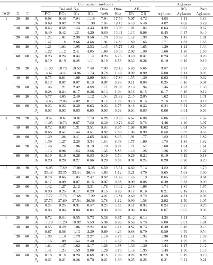
Remark 8. Belloni and Chernozhukov (2013) study post-model selection estimators which apply ordi-nary least squares to the model selected byfirst-step penalized estimators and show that the post Lasso estimators perform at least as well as Lasso in terms of the rate of convergence and have the advantage of having a smaller bias. After we apply our adaptive group Lasso procedure, we can re-estimate the panel data model based on the selected regressors and number of factors and the QMLE method of Bai (2009) or Moon and Weidner (2014a, 2014b). We will compare the performance of these post-Lasso estimators with the Lasso estimators through simulations.
Remark 9. Note that our asymptotic results are “pointwise” in the sense that the unknown parameters are treated asfixed. The implication is that infinite samples, the distributions of our estimators can be quite different from the normal, as discussed in Leeb and Pöscher (2005, 2008, 2009) and Schneider and Pöscher (2009). This is a well-known challenge in the literature of model selection no matter whether the selection is based on a information criterion or Lasso-type technique. Despite its importance, developing a thorough theory on uniform inference is beyond the scope of this paper.
Remark 10. As a referee kindly points out, our procedure does not take into account the possible correlation in and it may not work well in the case of strong serial correlation like Bai and Ng’s (2002) information criterion. Suppose that the error term has an AR(1) structure: =0−1+ where{ ≥1}is a white noise for each. Then one can transform the original model in (2.1) via the Cochrane and Orcutt’s (1949) procedure to obtain
−0−1=00¡−0−1¢+00˘0+ (3.3) where˘0 = ¡ 0 −00−1 ¢
We propose the following two-stage estimator:
Stage 1: Obtain the residuals ˆ using the largest model (i.e., = and including all regressors) and letˆbe the OLS estimator ofby regressingˆonˆ−1
Stage 2: Apply our Lasso method to the following transformed model:
(−ˆ−1) =00(−ˆ −1) +00˘0+ (3.4) whereis a new error term that incorporates both the original error term and the estimation error due to the replacement of0 byˆSimulations demonstrate such a method works fairly well in the case
3.4
Choosing the Tuning Parameter
LetS() and S() denote the index set of nonzero elements in ˆ()and nonzero columns in ˆ() respectively. LetS() =S()× S()Let|S|denote the cardinality of the index setSWe propose to select the tuning parameter= (1 2)by minimizing the following information criterion:
() = ˆ2() +1 |S()|+2 |S()| (3.5) where ˆ2() = L (ˆ()ˆ()) Similar information criteria are proposed by Wang et al. (2007) and Liao (2013) for shrinkage estimation in different contexts.
LetS ={1 }andS ={1 0}denote the index sets for the full set of covariates and the
(true) set of relevant covariates in respectively. Similarly, S={1 } andS ={1 0}
denote the index sets for the full set of factors and the (true) set of relevant factors in, respectively. LetS= (SS)be an arbitrary index set withS ={1 ∗}⊂S andS ={1 ∗}⊂S
where 0≤∗ ≤ and 0≤∗ ≤ Consider a candidate model with regressor index S and factor
indexS. Then any candidate model with eitherS+S orS+Sis referred to as anunder-fitted model in the sense that it misses at least one important covariate or factor. Similarly, any candidate model withS ⊃SS⊃Sand eitherS6=S orS6=S(i.e.,|S|+|S||S|+|S |)is referred as anover-fitted model in the sense that it contains not only all relevant covariates and factors but also at least one irrelevant covariate or factor.
DenoteΩ1= [0 1 max]andΩ2= [0 2 max]two bounded intervals inR+where the potential tuning
parameters1 and2 take values, respectively. Here we suppress the dependence ofΩ1Ω2 1 max
and2 maxon( )We divideΩ=Ω1×Ω2 into three subsetsΩ0Ω− andΩ+ as follows
Ω0 = {∈Ω:S() =S andS() =S}
Ω− = {∈Ω:S()+S orS()+S}
Ω+ = {∈Ω:S()⊃S,S()⊃S and |S|+|S||S |+|S |}
Clearly,Ω0Ω− and Ω+ denote the three subsets ofΩ in which the true, under- and over-fitted models
can be produced.
For any S = S × S with S = {1 |S|} ⊂ S and S = {1 |S|} ⊂ S we use
S = (1
|S|
)0 to denote an |S
| ×1 subvector of and S = (1 |S
|) to denote an
× |S|submatrix of . Similarly, S and ˆS denote the|S| ×1subvector of and |S| ×1
subvector of ˆ according toS LetˆS and ˆ
S denote the ordinary least squares (OLS) estimators of
S andS, respectively, by regressing onS andˆSDefine
ˆ 2S = 1 X =1 X =1 ³ −ˆ0SS−ˆ 0 S ˆ S ´2 (3.6)
whereˆ0S denotes the th row of ˆSLetS =S×S One can readily show thatˆ 2 S →2S ≡ lim()→∞ 1 P =1 P =1 ¡ 2 ¢
under Assumptions A.1-A.2. To proceed, we add the following two assumptions.
Assumption A.7For any S =S× S with eitherS +S or S+S there exists2S such that
ˆ
2S → 2
S 2S
Assumption A.8As( )→ ∞ 1 0→0 2 →0 1 2 → ∞and2 2 → ∞ Assumption A.7 is intuitively clear. It requires that all under-fitted models yield asymptotic mean square errors that are larger than 2
S, which is delivered by the true model. A.8 reflects the usual
conditions for the consistency of model selection. The penalty coefficients1 and2 cannot shrink to zero either too fast or too slowly.
Let0 = ¡ 0 1 02 ¢0where0
1 and02 satisfy the conditions on1 and2 , respectively in Assumptions A.3(ii)-(iii).
Theorem 3.5 Suppose that Assumptions A.1, A.2, A.3(i), A.6(i), A.7 and A.8 hold. Then
µ inf ∈Ω−∪Ω+ () ¡0 ¢ ¶ →1as ( )→ ∞
Remark 11. Note that we do not impose Assumptions A.3(ii)-(iii), A.4, A.5 and A.6(ii) in the above theorem. Theorem 3.5 implies that the ’s that yield the over- or under-selected sets of regressors or number of factors fail to minimize the information criterion w.p.a.1. Consequently, the minimizer of
() can only be the one that meets Assumptions A.3(ii)-(iii) so that both estimation and selection consistency can be achieved.
4
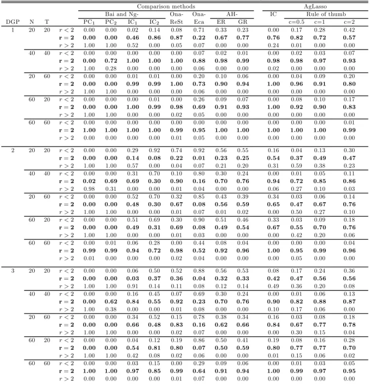
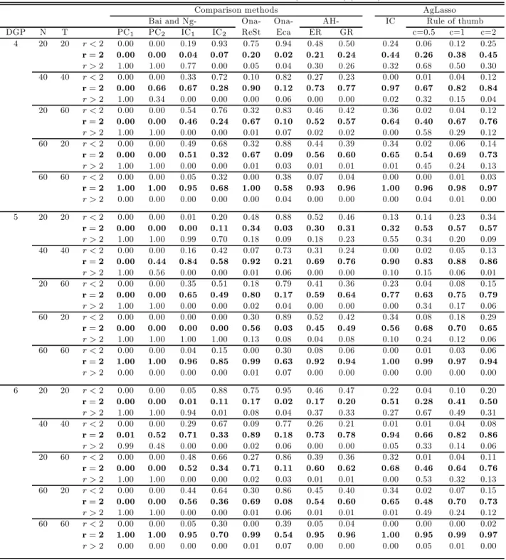
Monte Carlo Simulations
In this section, we conduct Monte Carlo simulations to evaluate the finite sample performance of our proposed adaptive group Lasso (agLasso) method.
4.1
Data Generating Processes
We consider the following data generating processes (DGPs): DGP 1: =0101+0202+ DGP 2: =011+022+0101+ 0 202+ where¡01 0 2 ¢ = (11) DGP 3: =011+02−1+0101+0202+ where ¡ 01 02¢= (1025) DGP 4: = 011+022+033+044 +055+0101 +0202 + where ¡ 01 02 03 04 05¢= (11000) DGP 5: = 011 +02−1 +032 +043 +05−2 +0101 +0202 + where ¡ 01 02 03 04 50¢= (1025000) DGP 6: =P=1 0 +0101+ 0 202+where ¡01 0 2 ¢ = (11),= 0 for= 3 and=b5( )15c
In all the six DGPs, 01 02 and are independent (01) random variables. In DGPs 1, 2, 4 and 6, 01 and 02 are independently and standard normally distributed. In DGPs 3 and 5, we
consider an AR(1) structure for the factors: 0
1 = 050−11+1 and 02 = 050−12+2, where
are IID (01) across both and for = 1 10 and the rest ’s are independent (01) for
= 11 (in DGP 6). We use to control for the signal-to-noise (SN) ratio, which is defined as Var¡00+000
¢
Var()For each DGP, we choose’s such that the SN ratio equals 1.6
DGP 1 is a pure factor structure without any regressor DGPs 2 and 3 are static and dynamic panel structures with interactivefixed effects, respectively. DGP 4 is identical to DGP 2 except that in DGP 4 we include three more irrelevant regressors: 3 4 and5. Hence, in DGP 4, we consider
both the selection of the regressors and determination of the number of factors, while in DGP 2 we only consider the latter. DGP 5 is identical to DGP 3, except that DGP 5 includes three irrelevant regressors:
2 3 and −2 Thus, we select both the regressors and number of factors in DGP 5. DGP 6 is
identical to DGPs 2 and 4 except that we consider a model with a growing number of regressors (), where =b5( )15c andb·c denotes the integer part of· Note that in this model, can be quite
large, e.g.,= 25when = 60and = 60
The true number of factors is 2 in all the above six DGPs. In our simulations, we assume that we do not know the true number of factors. We consider different combinations of( ) : (2020)(4040)
(2060),(6020)and(6060)The number of replications is 250.
4.2
Implementation
One of the important steps in our method is to choose the tuning parameters1 and2 . Following our theoretical arguments above, we use the information criterion in (3.5). Let 2
denote the sample variance of. For DGPs 1-3 where we only choose the number of factors, we set1 = 0and2 =
2
ln ( )(min ( )) For DGPs 4-6, we set 1 = 0052 ln ( )min ( ) and 2 =
2
ln ( )(min ( ))7 In DGPs 1-3, we only select factors, hence we let 1 = 0 and choose
2 from the set:©2 2
1 ( )−12(ln ( ))−1
ª
, where are50constants that increase geometri-cally from001to25i.e., = 0010014 18045and25For DGPs 4-5, we let the candidate set of
(1 2 )be the Cartesian product:{2( )−12(ln ( ))−1} ×{2 2
1 ( )−12(ln ( ))−1}
where are25constants that increase geometrically from001to258 We set1=2= 2 in all cases.
We also consider choices of (1 2 )based on a “rule of thumb” for DGPs 2-6:
(1 2 ) =·³2( )−12(ln ( ))−1 221 ( )−12(ln ( ))−1´
whereis a constant and we use the fact that and pass to infinity at the same rate and0 = 2is
fixed in DGPs 2-6. Of course, we reset1 = 0 for DGP 1. We consider three values for: 05 1and
2.
6The results for SN being 2 are reported in an early version of this paper and available upon request. 7A natural BIC-type choices of
1 and1 that satisfy Assumption A.8 would be1 =
2ln( ) 2 and2 = 2 ln( ) 2 Neverthess, in practice ln ( )− 2 = ln
min(12 12)max−1 −1is quite big in magnitude in
comparison with the usual BIC tuning coefficient ln ( )( )as denotes the total number of observations in our panel data model. Wefind that through simulations that a downward adjustment of the above1 by a scale of 1/10
would enhance thefinite sample performance of the proposed IC. That is why we choose to use1 = 005
2ln()
2
in our simulations and applications.
8To control the scale effect of the eigenvalues, we include2
1 in the2 Here we implicitly assume that there is at