Point triangulation through polyhedron collapse using the l∞ norm

(1)

Point triangulation through polyhedron collapse using the

`

∞

norm

Simon Donn´e, Bart Goossens, Wilfried Philips

Ghent University

iMinds-IPI-UGent

[email protected], [email protected], [email protected]

Abstract

Multi-camera triangulation of feature points based on a minimisation of the overall`2 reprojection error can get

stuck in suboptimal local minima or require slow global timisation. For this reason, researchers have proposed op-timising the`∞norm of the`2single view reprojection

er-rors, which avoids the problem of local minima entirely. In this paper we present a novel method for`∞triangulation that minimizes the`∞norm of the`∞reprojection errors: this apparently small difference leads to a much faster but equally accurate solution which is related to the MLE un-der the assumption of uniform noise. The proposed method adopts a new optimisation strategy based on solving sim-ple quadratic equations. This stands in contrast with the fastest existing methods, which solve a sequence of more complex auxiliary Linear Programming or Second Order Cone Problems. The proposed algorithm performs well: for triangulation, it achieves the same accuracy as existing techniques while executing faster and being straightforward to implement.

1. Introduction

Multiview triangulation is the problem of estimating the 3D location of a physical point from observations in multi-ple camera views. In low-commulti-plexity peomulti-ple tracking meth-ods for example, these feature points are the centroids of foreground blobs in a foreground/background segmented video sequence. In more complex methods, the features are computed using SURF [14] or similar detectors.

In realistic applications, confusion is possible between feature points corresponding to different points. This cor-respondence problem can be handled by grouped features according to their similarity and for each group triangulated the corresponding physical point. If the error of this tri-angulated point is too large, features are re-assigned after which the process is repeated until a satisfactory solution is reached. Clearly the performance of these methods depends crucially on that of the triangulation of separate points.

We propose a method based on minimizing the`∞norm of the`∞reprojection error, based on geometric insights of the 3D space. Each camerak∈ {1, . . . , K}has a camera-specific coordinate system defined by a rotation matrixRk

and a translationck. The relationship between the global

coordinatesr= (X, Y, Z)Tof a physical point and its coor-dinates in camerak’s reference systemrk= (Xk, Yk, Zk)

T

is given by the linear relationship rk(r) = Rkr +ck.

Assuming a pinhole camera model [10], the unknown r would – under ideal circumstances – be observed by cam-erakas a feature point with homogeneous pixel coordinates uk(r) = (xk(r), yk(r),1) = _X k(r) Zk(r), Yk(r) Zk(r),1 .

In reality – due to noisy observations – camerakwill ob-serve a feature at coordinatesu˜k = (˜xk,y˜k,1)rather than

the ideal coordinatesuk(r). The corresponding single view

reprojection errorγk(r)for camerakis

γk(r) 4

=ku˜k−uk(r)k, (1)

wherek.kis a suitably chosen norm.

Many methods in literature quantify the single view re-projection error in terms of the`2 norm, i.e. the euclidean

distance between the measurement and the reprojection of a hypothesized location. In this paper, we will however adopt the`∞norm:

γk(r) 4

= max(|˜xk−xk(r)|,|y˜k−yk(r)|). (2)

In any case, triangulation methods minimize the aggre-gatedreprojection error

γ(r) =k(γ1(r), . . . , γK(r))k. (3)

Traditionally, the`2norm is used to aggregate reprojection

errors. However,`∞methods use the `∞ norm instead – accordingly, so does our proposed method. Due to the non-linearity of the camera projection,γ(r)can have multiple local minima when defined in terms of the`2norm [2,6,9].

In contrast, aggregating the reprojection errors with the`∞ norm always results in a convex set of stationary points be-cause of its pseudo-convex character [1,3,5,12,16,17].

(2)

This absence of local minima ensures that local optimisa-tion methods converge to the global minimum ofγ(r).

Some existing methods use a mixed-norm: the`∞norm for aggregation but the `2 norm for the reprojection

er-ror [1,3,12,17]. Minimizing this aggregated error leads to a series of auxiliary second-order cone problems which are complex and time consuming to solve. More recent methods have evaluated the use of the `∞ norm for both the aggregated and the reprojection error (we will refer to this group as the full-`∞norm methods). This change al-lows expressing γ(r) as the point-wise maximum of lin-ear functions. Our proposed method will perform the op-timization by a series of line searches, and we show that our proposed method performs slightly faster than the exist-ing full-`∞norm methods, while arriving at the same opti-mum. Notably, our proposed method does not require any-thing more complex than the solution of one-dimensional quadratic equations and some basic matrix algebra.

Section2discusses existing triangulation methods, fol-lowed by a more detailed problem outline in section3after which we present the proposed method in section4. The re-sults in section5show that the proposed method is slightly faster than the state of the art methods while still achieving similar accuracy. Finally section6reaches the conclusion and we discuss possible future work in section7.

2. Existing work

Traditionally, triangulation methods employ the`2norm

for both the single view and aggregated reprojection er-ror. Minimizing this error corresponds to computing the maximum-likelihood estimate (MLE) under the assumption that the observed locations u˜k are perturbed by additive

white Gaussian noise (AWGN). Early methods [7,9,18] can get stuck in local minima caused by the non-linearity of the camera projection. Resolving this issue can be done through a (complex) branch-and-bound approach [11] or by solving for the entire set of stationary points [2].

But the problem of local minima can also be resolved by using the`∞norm in eq. (1): the so-called`∞methods which result in minimax problems. Olsson et al. [17] show that the resulting cost function – the point-wise maximum – is aquasi-convexfunction. This quasi-convexity implies that the set of stationary points is convex: no local optima exist. Yet even for many existing`∞methods, single view reprojection errors are expressed in terms of the `2 norm;

we will call themhybrid`∞methods [1,3,12,17]. We note that the criterion optimized by the hybrid approaches cannot easily be related to the maximum-likelihood estimation of a noise model.

In contrast to hybrid methods, we will express single view reprojection errors in terms of the`∞norm in this pa-per. As shown in the supplementary material, this full-`∞ norm method results in the maximum-likelihood estimation

under the assumption of uniform noise on the observations ˜

uk, lending a statistical foundation to the proposed method.

This norm was already studied in [5,16], with applications to large-dimensional multi-view geometry problems.

The hybrid methods result in the solution of a series of SOCP problems, which is time-consuming. In the semi-nal work of Kahl and Hartley [12] the bisection algorithm was introduced for optimizing the hybrid cost function. In the bisection algorithm a binary search narrows an inter-val containing the optimalγ? _{= arg min}

rγ(r). Olsson et al. [17] also propose an approach based on a series of auxil-iary problems, but not based on bisection: for their method, the auxiliary problems are local approximations to the origi-nal problem such that the KKT criteria are a simple approx-imation to the KKT criteria of the original problem. In [1], Agarwal et al. present a survey of the`∞ norm for aggre-gating reprojection errors. They present the Gugat method which outperforms the techniques of Olsson et al. [17] and Kahl [12] et al. while still being based on a series of SOCP problems. They also show the use of the`∞norm for ag-gregating and the`1 norm for the reprojection results in a

series of LP problems. Their method is still based on a se-ries of SOCP problems and is therefore only slightly faster than the methods by Olsson and Kahl. Finally, the authors of [3] show how the solution to the previous SOCP problem can be used as initialization to the next iteration’s problem in order to speed up the solver.

Recently, full-`∞ norm has garnered some attention. In [5], the authors propose a split-Bregman approach to the optimisation problem which results in an elegant modifica-tion of existing bundle adjustment (BA) packages. In each iteration of the algorithm, a single bundle adjustment it-eration is performed, as well as one evaluation of a prox-imal operator (which requires finding the root of a one-dimensional function). The authors show that it is faster than the Gugat method from [1], but it still requires the use of existing software packages such as SBA [13].

The authors of [16] use the full-`∞ norm as a way to detect outliers: handling the entire dataset as a single entity, outliers are removed based on their reprojection errors. We mention their approach here because it is an existing use of the full-`∞ norm, but the optimization is not continued beyond the removal of outliers.

In the proposed algorithm, we do not require a bisection algorithm, nor do we solve time-consuming auxiliary SOCP or BA problems. Rather, the proposed algorithm directly minimizes γ(r)through a sequence of line searches. The direction of the line search is computed in a straight forward manner conform the KKT conditions, and the line searches boil down to solving quadratic equations.

(3)

3. Background theory

We will adopt the common convention that only points in front of cameras are of interest, i.e.Zk(r)≥0for allk:

this is the so-called cheirality constraint from [8]. Taking into account thatrk =Zk(r)uk(r), it follows that

γk(r) =kZk(r) ˜uk−rk(r)k_∞/Zk(r). (4)

The objective of the proposed algorithm is to minimise γ(r): min r maxk γk(r). (5) Or equivalently to min r,γ γsubject toγ≥γk(r) ∀k. (6)

In order to remove the non-linearity of the constraints from the `∞ norm, we introduce the constant vectors i1 = (1,0,0)T,i2 = (−1,0,0)T,i3 = (0,1,0)T,i4 =

(0,−1,0)T_{. Using these notations, with}_k_{indexing the}_K

cameras andlindexing the vectorsil, the constraints can be

expressed as a set of linear inequalities: min r,γ γsubject to γ≥γk,l(r) 4 =i`·(rk(r)−Zk(r) ˜uk)/Zk(r) ∀k, l. ≡(γ+il·u˜k)Zk(r)≥il·rk(r),∀k, l. (7) AsZk(r)andrk(r)are linear functions ofrandu˜k is a

known constant vector, we can write that γk,l(r) =

a·r+b

c·r+d. (8) As shown by the authors of [17], such functions are all pseudo-convex. As a result the aggregated error – a point-wise maximum of these functions – is also pseudo-convex, implying that there are no local optima.

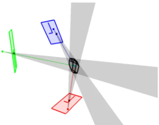
For a given value ofγ, the four constraints for a given camera define a pyramid in space, containing all points whose reprojection error for that camera is smaller thanγ. The feasible set for the constraints (7) is the intersection of the pyramids for all of the cameras, as shown in Fig-ure1this is a convex polyhedron. Our optimization algo-rithm iteratively reduces the value ofγuntil it approaches the optimal value γ?. This will cause this polyhedron to collapse onto itself: due to the quasi-convexity, each poly-hedron will be contained in the previous iteration’s polyhe-dron, and each of them will in turn contain the next step’s polyhedron and, eventually, the optimal pointr?_.

Figure 1. Example set-up. The cameras and their viewing planes are shown, as well as the pyramids they project in space for a given value ofγand the resulting polyhedron.

Over the course of the algorithm we compute improving directions in a sequence of pointsr(t)_{. In each subsequent}

point, one of the constraints is active (fulfilled with equal-ity), otherwise problem (7) would not be in its optimum. This also means that at each point of the iteration, the cur-rent location estimate lies on the hull of the polyhedron cor-responding to its`∞norm error. Because the optimum lies in the interior of the polyhedron, we select the improving direction in terms of the gradients of the active constraints, i.e. theinward-pointingnormal of the polyhedron faces in which the current estimate lies. In global coordinates these gradients are given by

gk,l(γ) = RTk −il+ (0,0, γ+il·u˜k)T

. (9)

4. Proposed approach

The algorithm starts with an arbitrary initial estimate r(0) _{of the sought position. We then iteratively select an}

improving direction and perform a line search. The only re-quirement for the initial point is that it must lie in front of all of the cameras (i.e. it satisfies the cheirality constraint).

In step(t)we define a polygon by usingγ =γ(r(t−1)₎

in equation (7). r(t−1) lies on the hull of this polygon, and due to pseudo-convexity the optimal pointr?_{must lie}

within the polyhedron. We select an improving direction d(t)(a direction pointing towards the interior of the polyhe-dron) and perform a line search along this direction. This process is repeated until the KKT constraints are fulfilled.

In practice, for example due to machine precision, some inequalities may only fulfil

γ(r)≈γk,l(r). (10)

We therefore evaluate whether constraints areactiveusing a threshold, i.e. by checking whether

(1−)γ(r)≤γk,l(r). (11)

(4)

4.1. Choice of improving direction

An improving direction points is computed in a point r(t−1). At least one constraint is active, i.e. r(t−1) lies on the surface of the polyhedron. Assuming that there are J active constraints, we will denote their normals byn1

throughnJ, in favour of brevity: which constraints

corre-spond to the various gradients is irrelevant for the following discussion.

In the case of a single active equality we simply select the normal of this active inequality as the improving direction: d(t)₌_n

1, which is simply the gradient descent approach.

Multiple active constraints complicate the direction choice, though. For two active constraints, r(t−1) _{lies on}

the edge of two faces of the polyhedron. The chosen direc-tion

d(t)=n1+n2 (12)

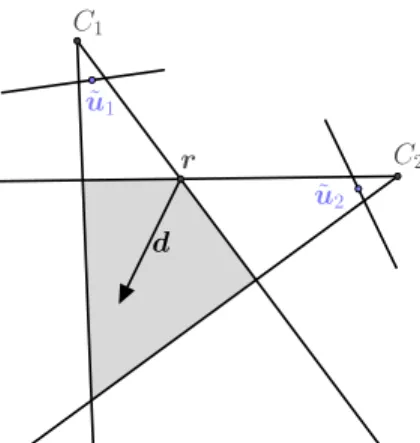
points along the interior angle bisector of the two faces and is orthogonal to the edge as shown for the two-dimensional case in figure2.

In case of three active constraints active,r(t−1)_{is a}

ver-tex of the polyhedron. The improving directiond(t)_is

con-structed as

d0 =n1×n2+n2×n3+n3×n1

s=n1·d/|n1·d|

d(t)=sd0 (13)

This is the vector with the same scalar product to all of the active constraint normals: the intersection of the pairwise face angle bisectors, where the signsis used to ensure that it points to the interior. In case the three normals are coplanar (the scalar product to any normal is zero), we test for each pair of normals whether their combination according to the previous paragraph violates the third normal, i.e. whether it has a negative dot product with this third normal. If and only if none of the pairs work, the algorithm terminates.

To handle cases of four or more active constraints, we investigate each of the possible triplets of active constraints and compute a candidate improving directiond(t)_{as before.}

If this candidate direction violates any of the constraints not included in the triplet, we select the next triplet and the pro-cess is repeated. If one of the triplets leads to termination of the algorithm or if none of the triplets lead to an improv-ing direction conform all of the constraints, it can be shown thatr(t−1)_{is optimal (see the supplementary material) and}

the algorithm terminates. The drawback is that all possi-ble triplets need to be examined. However, in the result section we show that the number of simultaneously active constraints is only very rarely higher than 3 or 4, such that this possibility only has a major influence.

C1 C2 ˜ u1 ˜ u2 r1= 0.23 r d

Figure 2. Illustration of the direction choice. The current estimate rand the improving directiondwhich is the sum of the gradients of each of the active constraints: the bisector for the corner.

In the supplementary material we show that the algo-rithm finishes (cannot find an improving direction) if and only if the KKT conditions are fulfilled. The current es-timate is then a stationary point and due to the pseudo-convexity of the cost function, this stationary point is a global optimum. Hence, the algorithm has indeed reached its goal.

4.2. Line search

After selecting the improving direction for iteration(t), we step to the pointr(t)₌_r(t−1)₊_α(t)_d(t)_{. For notational}

brevity, let fk,l(α) 4 =γk,l r(t−1)+αd(t). (14) For all active(k, l), _∂α∂ fk,l(α)

_α₌₀is negative. We choose

the master active constraint as the one with the least nega-tive value: the constraint which changes the least (and hence will remain active) for small steps along this line.

Now, let(k0, l0)be the master constraint and(k, l)any other (active or inactive) constraint. As (k0, l0) is active, fk0_,l0(α)is a decreasing function of αfor all α. On the

other hand, fk,l(α) may be increasing or decreasing and

may not even be monotonic. For α = 0, the activity of (k0, l0)implies thatfk,l(0) ≥ fk0_,l0(0). Locally, the error

for(k0, l0)is higher than the errors for all other constraints (k, l), but it decreases along the improving direction. At some value ofαthe graph may intersect with the graph of another constraint. Letαk,lbe the lowest strictly positive

value of alpha for whichfk0_,l0(α) =f_k,l(α), for any(k, l),

i.e. the point where another constraint mightbecome the new master constraint. As we know thatfk0_,l0(α)decreases

with increasing α, the pointr(t) ₌ _r(t−1)₊_α(t)_d(t) _is

guaranteed to have a lower reprojection error than r(t−1)_.

Finally, such an intersection is sure to exist if the direction points towards the interior of the polyhedron.

(5)

C

1

C

u

12

u

2

r

1

= 0

.

23

r(t−1)

r

2

= 0

.

09 r

3

= 0

.

02 t

e

1

g

1

h

1 r(t)

Figure 3. Example of the line search. Starting inr(t−1)_{, we step}

towardsr(t)so that it again lies on an edge of the polyhedron (the polygon in this 2D example). The unlabeled intermediate point lies only on an edge of the polyhedron and is rejected: we can still take a step along the improving direction without an increase in the cost function.

Evaluating the complementary constraint (the constraint corresponding to the same camera and the same coordinate as the master constraint, but the different sign) shows that it will always intersect forfk0_,l0(α) = 0, as that is where the

master constraint’s value equals that of its complementary constraint.

Now letα(t)_{= min}

k,lαk.l. This is the first point along

the line search after which the master constraintmight be-come inactive, and equivalently the first stationary point of the aggregated error along the search direction.

Equivalently, the selected value ofα(t)is the lowest pos-itive value for whichr(t)once again lies on an edge of the polyhedron as shown for two dimensions in Figure3(where an edge of the polyhedron in 3D becomes a vertex of the polyhedron in 2D). This edge is defined by the master con-straint and the concon-straint corresponding to the chosen value ofα. This implies that, except for the first iteration, the im-proving direction will always be chosen based on at least two active constraints.

As a final note, we discuss the computation ofαk,l by

solving the equation fk0_,l0(α) = f_k,l(α) for α, retaining

only the smallest positive solution. As either side is a frac-tion of linear funcfrac-tions ofα(see equation (8)), this equation is a quadratic equation in a single variable.

5. Results

5.1. Comparison of reprojection norms

The proposed cost function uses the `∞ norm in both the single view reprojection error and the aggregated error. Existing techniques for `∞ norm triangulation, however, sometimes use a mixed-norm: here we give a comparison between the optima of methods using`∞norm aggregation and either`1,`2or`∞norm reprojection errors.

0 0.01 0.02 0.03 0.04 0.05 0.06 0.07 0.08 0.09 Occurences Euclidean error (`∞,`∞) (`∞,`2) (`∞,`1) (`2,`2)

Figure 4. Accuracy for the various `∞-aggregation methods on synthetic data with Gaussian noise. The graph shows euclidean distances between the estimate and the ground truth.

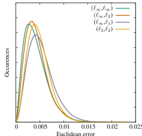
0 0.005 0.01 0.015 0.02 0.025 Occurences Euclidean error (`∞,`∞) (`∞,`2) (`∞,`1) (`2,`2)

Figure 5. Accuracy for the various `∞-aggregation methods on synthetic data with Gaussian noise. The graph shows euclidean distances between the estimate and the ground truth.

The test set-up consists of5random cameras observing a sequence of random points. We perturb the ideal obser-vations by the cameras either by additive white Gaussian noise or by additive white uniform noise. Figures4and5

show bezier-curves fitted to the histograms for the euclidean error between the triangulated points and the ground truth. Roughly, a heavier tail can be said to correspond to less robustness: large errors occur more often. We see a pre-dictable trend for the set with AWGN: the `∞ norm opti-mization is less robust than the`2norm. When adding

uni-form noise, the graph implies that the`∞norm aggregation and reprojection is the better choice: it is after all the MLE in that case (as shown in the supplementary material).

(6)

Occurences

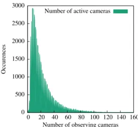
Number of observing cameras Number of active cameras

0 500 1000 1500 2000 2500 3000 0 20 40 60 80 100 120 140 160

Figure 6. Histogram of the number of cameras observing a single point for the ¨Orebro dataset.

5.2. Active inequalities and iterations

In order to illustrate the typically active number of con-straints, we will use the measurements of ¨Orebro Castle from [4]. This dataset is a collection of 761 views with a total of 58951 points visible in total, each visible in a sub-set of the views. In order to convey a sense of the number of views per point, we show a histogram of the number of cameras observing a point in figure6.

In figure7we illustrate the number of active inequalities in subsequent iterations of the algorithm. The first itera-tion only ever has a single active inequality (the initial point is very unlikely to lie on an edge of the polyhedron). Af-ter that, two or three active inequalities occur more or less equally often; four is much less likely (one to two orders of magnitude), while on the entire dataset only a single point (in a single iteration) had five active inequalities.

Finally, figure8illustrates the distribution of the number of iterations required for a point to reach convergence.

1 2 3 4 5 0 10 20 30 40 50 60 70 80 90 Acti v e inequalities Iteration log(Number)

Figure 7. Heatmap (in log-scale) for the number of active con-straints in a given iteration, normalized over the entire sequence.

Frequenc

y

Iterations until convergence

0 10 20 30 40 50 60 70 80 90

Figure 8. Distribution of the number of iterations required to reach convergence (over all points in the ¨Orebro dataset).

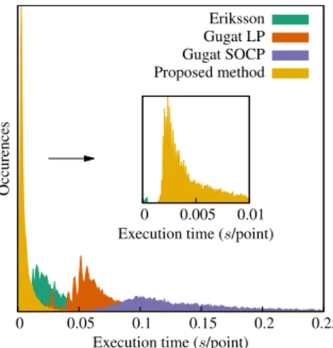
Occurences

Execution time (s/point) Execution time (s/point)

Eriksson Gugat LP Gugat SOCP Proposed method 0 0.05 0.1 0.15 0.2 0.25 0 0.005 0.01

Figure 9. Run times for discussed methods on synthetic data: 10000 points each visible in exactly 10 views.

5.3. Comparison of execution speed

In order to show that our technique is faster than ex-isting state-of-the-art methods for point triangulation, we compare with the Gugat algorithm from Agarwal [1] (both using the SOCP approach for the (`∞,`2) approach and the

LP approach resulting from the (`∞,`1)-mixed norm), and

the approach from Eriksson et al. [5] corresponding with the full-`∞approach. As a first evaluation, figure9shows the timing results on synthetic data with a fixed 10 viewpoints per point. In realistic datasets, the number of viewpoints per point is bound to change as not all cameras observe all points (see section5.2and in particular figure6).

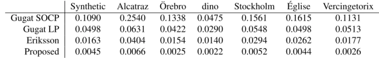
The first real dataset we compare with isdino.1 _{We also}

present results for the datasets of Alcatraz, ´Eglise du Dˆome, ¨

Orebro castle, Stockholm town hall and the Vercingetorix statue from [4] and [15]: the results for the datasets as shown in Figures10through15illustrate that our proposed method executes faster than the existing methods (sum-marised in Table 1). All of the techniques were evaluated in MATLAB using SeDuMi as the solver for the LP and SOCP problems [19], and SBA for bundle adjustment [13].

1

(7)

Occurences

Figure 10. Run times for discussed methods on the Alcatraz dataset with 65072 points over 419 views.

Occurences

Figure 11. Run times for discussed methods on thedinodataset with 4983 points over 36 views.

Occurences

Figure 12. Run times for discussed methods on the ´Eglise du Dˆome dataset with 84792 points over 85 views.

Occurences

Eriksson Gugat LP Gugat SOCP Proposed method 0 0.05 0.1 0.15 0.2 0 0.0025 0.005

Figure 13. Run times for discussed methods on the ¨Orebro Castle dataset with 59856 points over 761 views.

Occurences

Figure 14. Run times for discussed methods on the Stockholm Town Hall dataset with 28096 points over 43 views.

Occurences

Figure 15. Run times for discussed methods on the Vercingetorix statue dataset with 10789 points over 68 views.

(8)

Synthetic Alcatraz Orebro¨ dino Stockholm Eglise´ Vercingetorix Gugat SOCP 0.1090 0.2540 0.1338 0.0475 0.1561 0.1615 0.1131

Gugat LP 0.0498 0.0631 0.0422 0.0290 0.0548 0.0498 0.0513 Eriksson 0.0163 0.0404 0.0154 0.0140 0.0294 0.0262 0.0177 Proposed 0.0045 0.0066 0.0025 0.0022 0.0052 0.0044 0.0026

Table 1. Summary of the average execution times in seconds, over all datasets.

6. Conclusion

In this paper, we have proposed a novel technique of ap-proaching triangulation by using the`∞norm both for sin-gle view errors and the camera aggregation, resulting in a pseudo-convex problem without local minima.

The proposed method is based on geometrical interpre-tations of the cost function and its quasi-convexity of the objective function: the optimization can be seen as a series of polyhedrons representing a polyhedron collapsing onto itself until it has zero volume.

Our approach iteratively selects an improving direction and performs a line search along it. This is in contrast with the existing methods, which solve a sequence of complex problems. The less complex nature of the proposed ap-proach results in an easier-to-implement method, while per-forming faster (in contrast, existing methods use advanced solvers for their auxiliary problems). This leads us to be-lieve that a more efficient implementation would result in a larger speed benefit for the proposed method: the ex-isting methods are implemented largely with optimized li-braries while the proposed method was implemented solely in MATLAB.

7. Future Work

The presented work can be interpreted as the collapse of a polyhedron in 3D space. A promising avenue of future research is the use of this approach for the triangulation of volumes rather than points. We plan to expand this method such that general objects (which can be modelled by convex polyhedra) can be reconstructed efficiently: cameras often observe not a single point per object but rather a silhouette. We aim to generalise the proposed method in such a way as to enable an efficient polyhedral reconstruction of 3D ob-jects using the`∞norm.

References

[1] S. Agarwal, N. Snavely, and S. Seitz. Fast algorithms for l-infinity problems in multiview geometry. InComputer Vi-sion and Pattern Recognition, 2008. CVPR 2008. IEEE

Con-ference on, pages 1–8, June 2008.1,2,6

[2] M. Byrd, K. Josephson, and K. strm. Fast optimal three view triangulation. In Y. Yagi, S. Kang, I. Kweon, and H. Zha, ed-itors,Computer Vision ACCV 2007, volume 4844 ofLecture

Notes in Computer Science, pages 549–559. Springer Berlin

Heidelberg, 2007.1,2

[3] Z. Dai, Y. Wu, F. Zhang, and H. Wang. A novel fast method for l-infinity problems in multiview geometry. In A. Fitzgib-bon, S. Lazebnik, P. Perona, Y. Sato, and C. Schmid, edi-tors,Computer Vision ECCV 2012, volume 7576 ofLecture

Notes in Computer Science, pages 116–129. Springer Berlin

Heidelberg, 2012.1,2

[4] O. Enqvist, C. Olsson, and F. Kahl. Stable structure from motion using rotational consistency. Technical report, 2010. 6

[5] A. Eriksson and M. Isaksson. Pseudoconvex proximal split-ting for l-infinity problems in multiview geometry. In Com-puter Vision and Pattern Recognition (CVPR), 2014 IEEE

Conference on, pages 4066–4073, June 2014. 1,2,6

[6] R. Hartley, F. Kahl, C. Olsson, and Y. Seo. Verifying global minima for l2 minimization problems in multiple view geometry. International Journal of Computer Vision, 101(2):288–304, 2013.1

[7] R. Hartley and P. Sturm. Triangulation. pages 146–157, 1997.2

[8] R. I. Hartley. Cheirality invariants. InProceedings of DARPA

Image Understanding Workshop, pages 745–753, 1993.3

[9] R. I. Hartley and P. Sturm. Triangulation. Computer Vision

and Image Understanding, 68(2):146 – 157, 1997.1,2

[10] R. I. Hartley and A. Zisserman. Multiple View Geometry

in Computer Vision. Cambridge University Press, ISBN:

0521540518, second edition, 2004.1

[11] F. Kahl, S. Agarwal, M. Chandraker, D. Kriegman, and S. Belongie. Practical global optimization for multi-view geometry. International Journal of Computer Vision, 79(3):271–284, 2008.2

[12] F. Kahl and R. Hartley. Multiple-view geometry under the l-infinity norm. IEEE Trans. Pattern Anal. Mach. Intell., 30(9):1603–1617, Sept. 2008.1,2

[13] M. A. Lourakis and A. Argyros. SBA: A Software Package for Generic Sparse Bundle Adjustment. ACM Trans. Math.

Software, 36(1):1–30, 2009. 2,6

[14] D. H. Nga and K. Yanai. A spatio-temporal feature based on triangulation of dense surf. InComputer Vision Workshops

(ICCVW), 2013 IEEE International Conference on, pages

420–427, Dec 2013.1

[15] C. Olsson and O. Enqvist. Stable structure from motion for unordered image collections. In A. Heyden and F. Kahl, edi-tors,Image Analysis, volume 6688 ofLecture Notes in

Com-puter Science, pages 524–535. Springer Berlin Heidelberg,

2011.6

[16] C. Olsson, A. Eriksson, and R. Hartley. Outlier removal us-ing duality. In Computer Vision and Pattern Recognition

(CVPR), 2010 IEEE Conference on, pages 1450–1457, June

2010.1,2

[17] C. Olsson, A. Eriksson, and F. Kahl. Efficient optimization for l-problems using pseudoconvexity. InComputer Vision,

(9)

2007. ICCV 2007. IEEE 11th International Conference on, pages 1–8, Oct 2007.1,2,3

[18] H. Stewenius, F. Schaffalitzky, and D. Nister. How hard is 3-view triangulation really? InComputer Vision, 2005. ICCV

2005. Tenth IEEE International Conference on, volume 1,

pages 686–693 Vol. 1, Oct 2005.2

[19] J. Sturm. Using SeDuMi 1.02, a MATLAB toolbox for opti-mization over symmetric cones. Optimization Methods and

Software, 11–12:625–653, 1999. Version 1.05 available from