2
Fundamentals of Probability
and Statistics for Reliability
Analysis
∗
Assessment of the reliability of a hydrosystems infrastructural system or its components involves the use of probability and statistics. This chapter reviews and summarizes some fundamental principles and theories essential to relia-bility analysis.
2.1 Terminology
In probability theory, anexperiment represents the process of making obser-vations of random phenomena. The outcome of an observation from a random phenomenon cannot be predicted with absolute accuracy. The entirety of all possible outcomes of an experiment constitutes thesample space. Aneventis any subset of outcomes contained in the sample space, and hence an event could be an empty (or null) set, a subset of the sample space, or the sample space itself. Appropriate operators for events areunion, intersection, and com-plement. The occurrence of events AandB is denoted asA∪B(the union of A andB), whereas the joint occurrence of events Aand Bis denoted as A∩B or simply (A,B) (the intersection of AandB). Throughout the book, the comple-ment of eventAis denoted asA. When two eventsAandBcontain no common elements, then the two events aremutually exclusiveordisjoint events, which is expressed as (A,B)= ∅, where∅denotes the null set. Venn diagrams illustrat-ing the union and intersection of two events are shown in Fig. 2.1. When the oc-currence of eventAdepends on that of eventB, then they areconditional events,
∗Most of this chapter, except Secs. 2.5 and 2.7, is adopted from Tung and Yen (2005).
Figure 2.1 Venn diagrams for basic set operations.
which is denoted byA|B. Some useful set operation rules are 1. Commutative rule: A∪B =B∪A;A∩B=B∩A.
2. Associative rule: (A∪B)∪C= A∪(B∪C);(A∩B)∩C=A∩(B∩C). 3. Distributive rule: A∩(B∪C) = (A∩B)∪(A∩C);A∪(B∩C) = (A∪B)∩
(A∪C).
4. de Morgan’s rule: (A∪B)=A∩B;(A∩B)=A∪B.
Probabilityis a numeric measure of the likelihood of the occurrence of an event. Therefore, probability is a real-valued number that can be manipulated by ordinary algebraic operators, such as+,−,×, and/. The probability of the occurrence of an event Acan be assessed in two ways. In the case where an experiment can be repeated, the probability of having eventAoccurring can be estimated as the ratio of the number of replications in which event Aoccurs nAversus the total number of replicationsn, that is,nA/n. This ratio is called therelative frequencyof occurrence of eventAin the sequence ofnreplications. In principle, as the number of replications gets larger, the value of the relative
frequency becomes more stable, and the true probability of event Aoccurring could be obtained as
P(A)=limn→∞nAn (2.1)
The probabilities so obtained are calledobjectiveorposterior probabilities be-cause they depend completely on observations of the occurrence of the event.
In some situations, the physical performance of an experiment is prohibited or impractical. The probability of the occurrence of an event can only be estimated subjectively on the basis of experience and judgment. Such probabilities are calledsubjectiveorprior probabilities.
2.2 Fundamental Rules of Probability Computations 2.2.1 Basic axioms of probability
The three basic axioms of probability computation are (1)nonnegativity:P(A)≥ 0, (2)totality: P(S)=1, withSbeing the sample space, and (3)additivity: For two mutually exclusive events Aand B,P(A∪B)=P(A)+P(B).
As indicated from axioms (1) and (2), the value of probability of an event occurring must lie between 0 and 1. Axiom (3) can be generalized to consider K mutually exclusive events as
P(A1∪A2∪ · · · ∪AK)=P K ∪ k=1Ak = K k=1 P(Ak) (2.2)
Animpossible eventis an empty set, and the corresponding probability is zero, that is,P(∅)=0. Therefore, two mutually exclusive events AandB have zero probability of joint occurrence, that is,P(A,B)=P(∅)=0. Although the prob-ability of an impossible event is zero, the reverse may not necessarily be true. For example, the probability of observing a flow rate of exactly 2000 m3/s is zero, yet having a discharge of 2000 m3/s is not an impossible event.
Relaxing the requirement of mutual exclusiveness in axiom (3), the probabil-ity of the union of two events can be evaluated as
P(A∪B)=P(A)+P(B)−P(A,B) (2.3) which can be further generalized as
P K ∪ k=1 Ak = K k=1 P(Ak)− i< j P(Ai,Aj) + i< j <k P(Ai,Aj,Ak)− · · · +(−1)KP(A1,A2,. . .,AK) (2.4)
If all are mutually exclusive, all but the first summation term on the right-hand side of Eq. (2.3) vanish, and it reduces to Eq. (2.2).
Example 2.1 There are two tributaries in a watershed. From past experience, the probability that water in tributary 1 will overflow during a major storm event is 0.5, whereas the probability that tributary 2 will overflow is 0.4. Furthermore, the probability that both tributaries will overflow is 0.3. What is the probability that at least one tributary will overflow during a major storm event?
Solution Define Ei= event that tributary i overflows for i=1, 2. From the
prob-lem statements, the following probabilities are known:P(E1)=0.5,P(E2)=0.4, and
P(E1,E2)=0.3.
The probability having at least one tributary overflowing is the probability of event
E1orE2occurring, that is,P(E1∪E2). Since the overflow of one tributary does not
preclude the overflow of the other tributary,E1and E2are not mutually exclusive.
Therefore, the probability that at least one tributary will overflow during a major storm event can be computed, according to Eq. (2.3), as
P(E1∪E2)=P(E1)+P(E2)−P(E1,E2)=0.5+0.4−0.3=0.6
2.2.2 Statistical independence
If two events arestatistically independentof each other, the occurrence of one event has no influence on the occurrence of the other. Therefore, eventsAandB are independent if and only if P(A,B) = P(A)P(B). The probability of joint occurrence ofK independent events can be generalized as
P K ∩ k=1Ak =P(A1)×P(A2)× · · · ×P(AK)= K k=1 P(Ak) (2.5)
It should be noted that the mutual exclusiveness of two events does not, in general, imply independence, and vice versa, unless one of the events is an impossible event. If the two events Aand B are independent, then A,A,B, andBall are independent, but not necessarily mutually exclusive, events.
Example 2.2 Referring to Example 2.1, the probabilities that tributaries 1 and 2 overflow during a major storm event are 0.5 and 0.4, respectively. For simplicity, assume that the occurrences of overflowing in the two tributaries are independent of each other. Determine the probability of at least one tributary overflowing in a major storm event.
Solution Use the same definitions for eventsE1andE2. The problem is to determine
P(E1∪E2) by
P(E1∪E2)=P(E1)+P(E2)−P(E1,E2)
Note that in this example the probability of joint occurrences of both tributaries
over-flowing, that is, P(E1,E2), is not given directly by the problem statement, as in
overflows in the tributaries are independent events, according to Eq. (2.5), as
P(E1,E2)= P(E1)P(E2)=(0.5)(0.4)=0.2
Then the probability that at least one tributary would overflow during a major storm event is
P(E1∪E2)=P(E1)+P(E2)−P(E1,E2)=0.5+0.4−0.2=0.7
2.2.3 Conditional probability
Theconditional probabilityis the probability that a conditional event would occur. The conditional probability P(A|B) can be computed as
P(A|B)= P(A,B)
P(B) (2.6)
in which P(A|B) is the occurrence probability of event Agiven that eventB has occurred. It represents a reevaluation of the occurrence probability of event Ain the light of the information that eventB has occurred. Intuitively, Aand Bare two independent events if and only if P(A|B)=P(A). In many cases it is convenient to compute the joint probabilityP(A,B) by
P(A,B)=P(B)P(A|B) or P(A,B)=P(A)P(B|A)
The probability of the joint occurrence ofK dependent events can be general-ized as P K ∩ k=1Ak =P(A1)×P(A2|A1)×P(A3|A2,A1)×· · ·×P(AK|AK−1,. . .,A2,A1) (2.7) Example 2.3 Referring to Example 2.2, the probabilities that tributaries 1 and 2 would overflow during a major storm event are 0.5 and 0.4, respectively. After exam-ining closely the assumption about the independence of overflow events in the two tributaries, its validity is questionable. Through an analysis of historical overflow events, it is found that the probability of tributary 2 overflowing is 0.6 if tributary 1 overflows. Determine the probability that at least one tributary would overflow in a major storm event.
Solution Let E1and E2be the events that tributary 1 and 2 overflow, respectively. From the problem statement, the following probabilities can be identified:
P(E1)=0.5 P(E2)=0.4 P(E2|E1)=0.6
in which P(E2|E1) is the conditional probability representing the likelihood that
tributary 2 would overflow given that tributary 1 has overflowed. The probability of at least one tributary overflowing during a major storm event can be computed by
in which the probability of joint occurrence of both tributaries overflowing, that
is, P(E1,E2), can be obtained from the given conditional probability, according to
Eq. (2.7), as
P(E1,E2)= P(E2|E1)P(E1)=(0.6)(0.5)=0.3
The probability that at least one tributary would overflow during a major storm event can be obtained as
P(E1∪E2)=P(E1)+P(E2)−P(E1,E2)=0.5+0.4−0.3=0.6
2.2.4 Total probability theorem and Bayes’ theorem
The probability of the occurrence of an event E, in general, cannot be deter-mined directly or easily. However, the event E may occur along with other attribute events Ak. Referring to Fig. 2.2, event Ecould occur jointly with K mutually exclusive (Aj ∩Ak= ∅for j=k) andcollectively exhaustive(A1∪A2 ∪ · · · ∪AK)=SattributesAk,k=1, 2,. . .,K. Then the probability of the occur-rence of an eventE, regardless of the attributes, can be computed as
P(E)= K k=1 P(E,Ak)= K k=1 P(E|Ak)P(Ak) (2.8)
Equation (2.8) is called thetotal probability theorem.
Example 2.4 Referring to Fig. 2.3, two upstream storm sewer branches (I1and I2)
merge to a sewer main (I3). Assume that the flow-carrying capacities of the two
up-stream sewer branchesI1 and I2 are equal. However, hydrologic characteristics of
the contributing drainage basins corresponding to I1 and I2 are somewhat
differ-ent. Therefore, during a major storm event, the probabilities that sewersI1and I2
will exceed their capacities (surcharge) are 0.5 and 0.4, respectively. For simplicity, assume that the occurrences of surcharge events in the two upstream sewer branches
are independent of each other. If the flow capacity of the downstream sewer mainI3is
A1
S
A2 A3 A4
E
Figure 2.2 Schematic diagram of total probability theorem.
1 2
3
Figure 2.3 A system with three sewer sections.
the same as its two upstream branches, what is the probability that the flow capacity
of the sewer mainI3will be exceeded? Assume that when both upstream sewers are
carrying less than their full capacities, the probability of downstream sewer mainI3
exceeding its capacity is 0.2.
Solution LetE1,E2, and E3, respectively, be events that sewer I1,I2, andI3exceed their respective flow capacity. From the problem statements, the following
probabili-ties can be identified:P(E1)=0.50,P(E2)=0.40, andP(E3|E1,E2)=0.2.
To determineP(E3), one first considers the basic events occurring in the two
up-stream sewer branches that would result in surcharge in the downup-stream sewer main
E3. There are four possible attribute events that can be defined from the flow
con-ditions of the two upstream sewers leading to surcharge in the downstream sewer
main. They are A1=(E1,E2),A2=(E1,E2), A3=(E1,E2), andA4=(E1,E2).
Fur-thermore, the four eventsA1,A2,A3, andA4are mutually exclusive.
Since the four attribute events A1, A2, A3, and A4 contribute to the occurrence
of eventE3, the probability of the occurrence of E3can be calculated, according to
Eq. (2.8), as
P(E3) = P(E3,A1)+P(E3,A2)+P(E3,A3)+P(E3,A4)
= P(E3|A1)P(A1)+P(E3|A2)P(A2)+P(E3|A3)P(A3)+P(E3|A4)P(A4)
To solve this equation, each of the probability terms on the right-hand side must
be identified. First, the probability of the occurrence of A1, A2, A3, and A4 can be
determined as the following:
P(A1)=P(E1,E2)= P(E1)×P(E2)=(0.5)(0.4)=0.2
The reason thatP(E1,E2)=P(E1)×P(E2) is due to the independence of eventsE1
independent events. Therefore,
P(A2)= P(E1,E2)=P(E1)×P(E2)=(1−0.5)(0.4)=0.2
P(A3)= P(E1,E2)=P(E1)×P(E2)=(0.5)(1−0.4)=0.3
P(A4)= P(E1,E2)=P(E1)×P(E2)=(1−0.5)(1−0.4)=0.3
The next step is to determine the values of the conditional probabilities, that is, P(E3|A1),P(E3|A2),P(E3|A3), andP(E3|A4). The value ofP(E3|A4)=P(E3|E1,
E2) =0.2 is given by the problem statement. On the other hand, the values of the
remaining three conditional probabilities can be determined from an understanding of the physical process. Note that from the problem statement the downstream sewer main has the same conveyance capacity as the two upstream sewers. Hence any up-stream sewer exceeding its flow-carrying capacity would result in surcharge in the downstream sewer main. Thus the remaining three conditional probabilities can be easily determined as
P(E3|A1) = P(E3|E1,E2)=1.0
P(E3|A2) = P(E3|E1,E2)=1.0
P(E3|A3) = P(E3|E1,E2)=1.0
Putting all relevant information into the total probability formula given earlier, the
probability that the downstream sewer main I3 would be surcharged in a major
storm is
P(E3)= P(E3|A1)P(A1)+P(E3|A2)P(A2)+P(E3|A3)P(A3)+P(E3|A4)P(A4)
=(1.0)(0.2)+(1.0)(0.2)+(1.0)(0.3)+(0.2)(0.3)
=0.76
The total probability theorem describes the occurrence of an event E that may be affected by a number of attribute events Ak,k=1, 2,. . .,K. In some situations, one knows P(E|Ak) and would like to determine the probability that a particular event Ak contributes to the occurrence of event E. In other words, one likes to find P(Ak|E). Based on the definition of the conditional probability (Eq. 2.6) and the total probability theorem (Eq. 2.8),P(Ak|E) can be computed as P(Ak|E)= P(Ak,E) P(E) = P(E|Ak)P(Ak) K k=1P(E|Ak)P(Ak) fork=1, 2,. . .,K (2.9)
Equation (2.9) is calledBayes’ theorem, andP(Ak) is theprior probability, rep-resenting the initial belief of the likelihood of occurrence of attribute eventAk. P(E|Ak) is thelikelihood function, andP(Ak|E) is theposterior probability, representing the new evaluation ofAk being responsible in the light of the oc-currence of event E. Hence Bayes’ theorem can be used to update and revise the calculated probability as more information becomes available.
Example 2.5 Referring to Example 2.4, if surcharge is observed in the downstream
storm sewer mainI3, what is the probability that the incident is caused by
simulta-neous surcharge of both upstream sewer branches?
Solution From Example 2.4,A1represents the event that both upstream storm sewer branches exceed their flow-carrying capacities. The problem is to find the conditional
probability ofA1, given that event E3has occurred, that is,P(A1|E3). This
condi-tional probability can be expressed as P(A1|E3)=
P(A1,E3)
P(E3)
= P(E3|A1)P(A1)
P(E3)
From Example 2.4, the numerator and denominator of the preceding conditional prob-ability can be computed as
P(A1|E3)=
P(E3|A1)P(A1)
P(E3) =
(1.0)(0.2)
0.76 =0.263
The original assessment of the probability is 20 percent that both upstream sewer branches would exceed their flow-carrying capacities. After an observation of down-stream surcharge from a new storm event, the probability of surcharge occurring in both upstream sewers is revised to 26.3 percent.
2.3 Random Variables and their Distributions
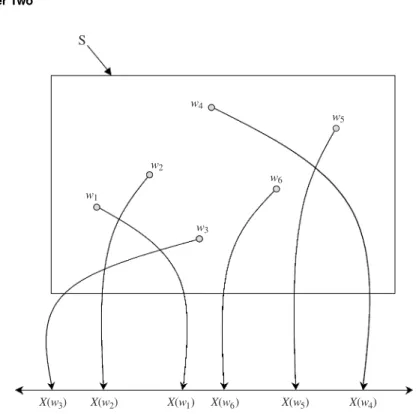
In analyzing the statistical features of infrastructural system responses, many events of interest can be defined by the related random variables. Arandom variableis a real-value function defined on the sample space. In other words, a random variable can be viewed as a mapping from the sample space to the real line, as shown in Fig. 2.4. The standard convention is to denote a random variable by an upper-case letter, whereas a lower-case letter is used to repre-sent the realization of the corresponding random variable. For example, one may useQto represent flow magnitude, a random variable, whereasqis used to represent the values thatQtakes. A random variable can be discrete or con-tinuous. Examples of discrete random variables encountered in hydrosystems infrastructural designs are the number of storm events occurring in a specified time period, the number of overtopping events per year for a levee system, and so on. On the other hand, examples of continuous random variables are flow rate, rainfall intensity, water-surface elevation, roughness factor, and pollution concentration, among others.
2.3.1 Cumulative distribution function and probability density function
The cumulative distribution function (CDF), or simply distribution function (DF), of a random variableXis defined as
X(w3) S X(w2) X(w1) X(w6) X(w5) X(w4) w3 w2 w1 w4 w6 w5
Figure 2.4 A random variableX(w) as mapped from the sample space to the real line.
The CDF Fx(x) is the nonexceedance probability, which is a nondecreasing function of the argumentx, that is,Fx(a)≤ Fx(b), fora<b. As the argument x approaches the lower bounds of the random variable X, the value of Fx(x) approaches zero, that is, limx→−∞Fx(x) = 0; on the other hand, the value of
Fx(x) approaches unity as its argument approaches the upper bound ofX, that is, limx→∞Fx(x)=1. Witha<b,P(a<X≤b)=Fx(b)−Fx(a).
For a discrete random variable X, the probability mass function(PMF), is defined as
px(x)=P(X =x) (2.11)
The PMF of any discrete random variable, according to axioms (1) and (2) in Sec. 2.1, must satisfy two conditions: (1) px(xk) ≥ 0, for all xk’s, and (2)
allkpx(xk) = 1. The PMF of a discrete random variable and its associated CDF are sketched schematically in Fig. 2.5. As can be seen, the CDF of a dis-crete random variable is a staircase function.
For a continuous random variable, the probability density function (PDF) fx(x) is defined as
fx(x)=
dFx(x)
px(x x ) x x1 x2 x3 xK−1 xK 1 (a) (b) x1 x2 x3 x xK 0 x F(x) K−1
Figure 2.5 (a) Probability mass function (PMF) and (b) cumulative distribution function (CDF) of a discrete random variable.
The PDF of a continuous random variable fx(x) is the slope of its corresponding CDF. Graphic representations of a PDF and a CDF are shown in Fig. 2.6. Similar to the discrete case, any PDF of a continuous random variable must satisfy two conditions: (1) fx(x) ≥ 0 and (2)
fx(x)dx = 1. Given the PDF of a random variableX, its CDF can be obtained as
Fx(x)=
x
−∞
fx(u)du (2.13)
in whichuis the dummy variable. It should be noted that fx(·) is not a prob-ability; it only has meaning when it is integrated between two points. The probability of a continuous random variable taking on a particular value is zero, whereas this may not be the case for discrete random variables.
1 Fx(x) 0 x fx(x) 0 x (b) (a)
Figure 2.6 (a) Probability density function (PDF) and (b) cu-mulative distribution function (CDF) of a continuous random variable.
Example 2.6 The time to failureT of a pump in a water distribution system is a continuous random variable having the PDF of
ft(t)=exp(−t/1250)/β fort≥0, β >0
in whichtis the elapsed time (in hours) before the pump fails, andβis the parameter
of the distribution function. Determine the constantβand the probability that the
operating life of the pump is longer than 200 h.
Solution The shape of the PDF is shown in Fig. 2.7. If the function ft(t) is to serve as
a PDF, it has to satisfy two conditions: (1) ft(t)≥0, for allt, and (2) the area under
ft(t) must equal unity. The compliance of the condition (1) can be proved easily. The
value of the constantβcan be determined through condition (2) as
1= ∞ 0 ft(t)dt= ∞ 0 e−t/1250 β dt= −1250e−t/1250 β ∞ 0 = 1250β
ft(t)
0 t
1/b
Time-to-failure, t
ft(t) = (1/b)e–t/b
Figure 2.7 Exponential failure density curve.
Therefore, the constantβ=1250 h/failure. This particular PDF is called the
exponen-tial distribution(see Sec. 2.6.3). To determine the probability that the operational life
of the pump would exceed 200 h, one calculatesP(T ≥200):
P(T ≥200)= ∞ 200 e−t/1250 1250 dt= −e−t/1250∞ 200=e− 200/1250=0.852
2.3.2 Joint, conditional, and marginal distributions
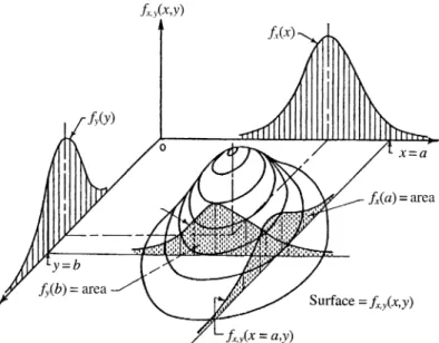
Thejoint distributionandconditional distribution, analogous to the concepts of joint probability and conditional probability, are used for problems involving multiple random variables. For example, flood peak and flood volume often are considered simultaneously in the design and operation of a flood-control reservoir. In such cases, one would need to develop ajoint PDFof flood peak and flood volume. For illustration purposes, the discussions are limited to problems involving two random variables.
Thejoint PMFandjoint CDFof two discrete random variablesX andY are defined, respectively, as px,y(x,y)= P(X=x,Y =y) (2.14a) Fx,y(u,v)= P(X≤u,Y ≤v)= x≤u y≤v px,y(x,y) (2.14b)
Schematic diagrams of the joint PMF and joint CDF of two discrete random variables are shown in Fig. 2.8.
0.3 0.1 0.1 0.1 0.2 0.2 y x x1 x2 x3 x1 x2 x3 y2 y1 1.0 0.7 y 0.3 0.4 0.2 0.1 y2 y1 (b) (a) x Fx,y(x,y) px,y(x,y)
Figure 2.8 (a) Joint probability mass function (PMF) and (b) cumula-tive distribution function (CDF) of two discrete random variables.
The joint PDF of two continuous random variables X and Y, denoted as fx,y(x,y), is related to its corresponding joint CDF as
fx,y(x,y)= ∂ 2[F x,y(x,y)] ∂x∂y (2.15a) Fx,y(x,y)= x −∞ y −∞ fx,y(u,v)du d v (2.15b)
Similar to the univariate case,Fx,y(−∞,−∞)=0 andFx,y(∞,∞)=1. Two ran-dom variablesX andY are statistically independent if and only if fx,y(x,y)= fx(x)× fy(y) andFx,y(x,y)=Fx(x)×Fy(y). Hence a problem involving multi-ple independent random variables is, in effect, a univariate problem in which each individual random variable can be treated separately.
If one is interested in the distribution of one random variable regardless of all others, themarginal distributioncan be used. Given the joint PDF fx,y(x,y), themarginal PDFof a random variable Xcan be obtained as
fx(x)=
∞
−∞ fx,y(x,y)dy (2.16)
For continuous random variables, theconditional PDFforX|Y, similar to the conditional probability shown in Eq. (2.6), can be defined as
fx(x|y)=
fx,y(x,y) fy(y)
(2.17) in which fy(y) is the marginal PDF of random variableY. The conditional PMF for two discrete random variables similarly can be defined as
px(x|y)= px,y(x,y)
py(y) (2.18)
Figure 2.9 shows the joint and marginal PDFs of two continuous random vari-ablesXandY. It can be shown easily that when the two random variables are statistically independent, fx(x|y)= fx(x).
Equation (2.17) alternatively can be written as
fx,y(x,y)=fx(x|y)× fy(y) (2.19) which indicates that a joint PDF between two correlated random variables can be formulated by multiplying a conditional PDF and a suitable marginal PDF.
Figure 2.9 Joint and marginal probability density function (PDFs) of two continuous random variables. (After Ang and Tang, 1975.)
Note that the marginal distributions can be obtained from the joint distribution function, but not vice versa.
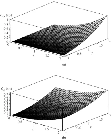
Example 2.7 Suppose that X andY are two random variables that can only take
values in the intervals 0≤ x ≤2 and 0≤ y≤ 2. Suppose that the joint CDF of X
andY for these intervals has the form of Fx,y(x,y)=cxy(x2+y2). Find (a) the joint
PDF ofXandY, (b) the marginal PDF ofX, (c) the conditional PDF fy(y|x=1), and
(d)P(Y ≤1|x=1).
Solution First, one has to find the constantcso that the functionFx,y(x,y) is a
legit-imate CDF. It requires that the value ofFx,y(x,y)=1 when both arguments are at
their respective upper bounds. That is,
Fx,y(x=2, y=2)=1=c(2)(2)(22+22)
Therefore,c=1/32. The resulting joint CDF is shown in Fig. 2.10a.
1 0.8 0.6 0.4 0.2 0 0 0 (a) 0.5 0.5 1.5 Fx,y(x,y) 1.5 1 1 2 2 0.6 0.7 0.5 0.4 0.3 0.2 0.1 0 0 0 (b) 0.5 0.5 1.5 fx,y(x,y) 1.5 1 1 2 2 x y x y
Figure 2.10 (a) Joint cumulative distribution function (CDF) and (b) probability density function (PDF) for Example 2.7.
(a) To derive the joint PDF, Eq. (2.15a) is applied, that is, fx,y(x,y)=∂∂ x ∂ ∂y xy(x2+y2) 32 = ∂ ∂x x3+3xy2 32 =3(x2+y2) 32 for 0≤x, y≤2
A plot of joint PDF is shown in Fig. 2.10b.
(b) To find the marginal distribution ofX, Eq. (2.16) can be used:
fx(x)= 2 0 3(x2+y2) 32 dx= 4+3x2 16 for 0≤x≤2
(c) The conditional distribution fy(y|x) can be obtained by following Eq. (2.17) as
fy(y|x=1)= fx,y(x=1,y) fx(x=1) = 3[(1)2+y2] 32 4+3(1)2 16 =3(1+y2) 14 for 0≤y≤2
(d) The conditional probabilityP(Y ≤1|X=1) can be computed as
P(Y ≤1|X=1)= 1 0 fy(y|x=1)dy= 1 0 3(1+y2) 14 dy= 2 7
2.4 Statistical Properties of Random Variables
In statistics, the termpopulationis synonymous with the sample space, which describes the complete assemblage of all the values representative of a partic-ular random process. Asampleis any subset of the population. Furthermore, parametersin a statistical model are quantities that are descriptive of the pop-ulation. In this book, Greek letters are used to denote statistical parameters. Sample statistics, or simplystatistics, are quantities calculated on the basis of sample observations.
2.4.1 Statistical moments of random variables
In practical statistical applications, descriptors commonly used to show the sta-tistical properties of a random variable are those indicative of (1) the central tendency, (2) the dispersion, and (3) the asymmetry of a distribution. The fre-quently used descriptors in these three categories are related to thestatistical momentsof a random variable. Currently, two types of statistical moments are used in hydrosystems engineering applications: product-moments and L-moments. The former is a conventional one with a long history of practice, whereas the latter has been receiving great attention recently from water re-sources engineers in analyzing hydrologic data (Stedinger et al., 1993; Rao and Hamed 2000). To be consistent with the current general practice and usage, the termsmomentsandstatistical momentsin this book refer to the conventional product-moments unless otherwise specified.
Product-moments. Therth-orderproduct-momentof a random variableXabout any reference pointX=xois defined, for the continuous case, as
E[(X−xo)r]= ∞ −∞(x−xo) rf x(x)dx= ∞ −∞(x−xo) rdF x(x) (2.20a) whereas for the discrete case,
E[(X−xo)r]= K
k=1
(xk−xo)rpx(xk) (2.20b)
where E[·] is astatistical expectation operator. In practice, the first three mo-ments (r=1, 2, 3) are used to describe the central tendency, variability, and asymmetry of the distribution of a random variable. Without losing generality, the following discussions consider continuous random variables. For discrete random variables, the integral sign is replaced by the summation sign. Here it is convenient to point out that when the PDF in Eq. (2.20a) is replaced by a conditional PDF, as described in Sec. 2.3, the moments obtained are called the conditional moments.
Since the expectation operatorE[·] is for determining the average value of the random terms in the brackets, the sample estimator for the product-moments forµr=E(Xr), based onnavailable data (x1,x2,. . .,xn), can be written as
µ r= n i=1 wi(n)xir (2.21)
wherewi(n) is a weighting factor for sample observationxi, which depends on sample sizen. Most commonly,wi(n)=1/n, for alli=1, 2,. . .,n. The last column of Table 2.1 lists the formulas applied in practice for computing some commonly used statistical moments.
Two types of product-moments are used commonly:moments about the ori-gin, where xo=0, and central moments, where xo=µx, with µx=E[X]. The rth-order central moment is denoted as µr=E[(X −µx)r], whereas ther th-order moment about the origin is denoted asµr =E(Xr). It can be shown easily, through thebinomial expansion, that the central momentsµr=E[(X−µx)r] can be obtained from the moments about the origin as
µr= r
i=0
(−1)iCr,iµixµr−i (2.22)
whereCr,i =ri=i!(rr−!i)! is abinomial coefficient, with ! representing factorial, that is,r!=r ×(r −1)×(r−2)× · · · ×2×1. Conversely, the moments about the origin can be obtained from the central moments in a similar fashion as
µ r= r i=0 Cr,iµixµr−i (2.23)
T ABLE 2.1 Pr oduct-Moments of Random V ariab les Moment Measure of De fi nition Continuous variable Discrete variable Sample estimator F irst Central Mean, expected value µx = ∞ −∞ xf x ( x ) dx µx = all x s xk p ( xk ) ¯ x = xi / n location E ( X ) = µx Second Dispersion V ariance , V ar( X ) = µ2 = σ 2 x σ 2=x ∞ −∞ ( x − µx ) 2f x ( x ) dx σ 2=x all x s ( xk − µx ) 2P x ( xk ) s 2= 1 n − 1 ( xi − ¯ x ) 2 Standard deviation, σx σx = V ar( X ) σx = V ar( X ) s = 1 n − 1 ( xi − ¯ x ) 2 Coef fi cient of variation, x x = σx /µ x x = σx /µ x Cv = s / ¯ x Third Asymmetry Skewness µ3 = ∞ −∞ ( x − µx ) 3f x ( x ) dx µ3 = all x s ( xk − µx ) 3p x ( xk ) m3 = n ( n − 1) ( n − 2) ( xi − ¯ x ) 3 Skewness coef fi cient, γx γx = µ3 /σ 3 x γx = µ3 /σ 3 x g = m3 / s 3 F ourth P eakedness Kurtosis , κx µ4 = ∞ −∞ ( x − µx ) 4f x ( x ) dx µ4 = all x s ( xk − µx ) 4p x ( xk ) m4 = n ( n + 1) ( n − 1) ( n − 2) ( n − 3) ( xi − ¯ x ) 4 Excess coef fi cient, εx κx = µ4 /σ 4 x κx = µ4 /σ 4 x k = m4 / s 4 εx = κx − 3 εx = κx − 3 37
Equation (2.22) enables one to compute central moments from moments about the origin, whereas Eq. (2.23) does the opposite. Derivations for the expressions of the first four central moments and the moments about the origin are left as exercises (Problems 2.10 and 2.11).
The main disadvantages of the product-moments are (1) that estimation from sample observations is sensitive to the presence of extraordinary values (called outliers) and (2) that the accuracy of sample product-moments deteriorates rapidly with an increase in the order of the moments. An alternative type of moments, calledL-moments, can be used to circumvent these disadvantages.
Example 2.8 (after Tung and Yen, 2005) Referring to Example 2.6, determine the first two moments about the origin for the time to failure of the pump. Then calculate the first two central moments.
Solution From Example 2.6, the random variableT is the time to failure having an exponential PDF as ft(t)= 1 β exp(−t/1250) fort≥0, β >0
in whichtis the elapsed time (in hours) before the pump fails, andβ=1250 h/failure.
The moments about the origin, according to Eq. (2.20a), are E(Tr)=µr= ∞ 0 tr e−t/β β dt
Using integration by parts, the results of this integration are
forr=1, µ1=E(T)=µt=β=1250 h
forr=2, µ2=E(T2)=2β2=3,125,000 h2
Based on the moments about the origin, the central moments can be determined, according to Eq. (2.22) or Problem (2.10), as
forr=1, µ1=E(T −µt)=0
forr=2, µ2=E[(T −µt)2]=µ2−µ2=2β2−β2=β2=1, 562, 500 h2
L-moments. Therth-orderL-momentsare defined as (Hosking, 1986, 1990)
λr= 1 r r−1 j=0 (−1)j r −1 j E(Xr−j:r) r=1, 2,. . . (2.24)
in which Xj:n is the jth-order statisticof a random sample of sizenfrom the distribution Fx(x), namely, X(1) ≤ X(2) ≤ · · · ≤ X(j) ≤ · · · · ≤ X(n). The “L” in L-moments emphasizes thatλris a linear function of the expected order statis-tics. Therefore, sample L-moments can be made a linear combination of the ordered data values. The definition of the L-moments given in Eq. (2.24) may appear to be mathematically perplexing; the computations, however, can be sim-plified greatly through their relations with theprobability-weighted moments,
which are defined as (Greenwood et al., 1979) Mr,p,q=E{Xr[Fx(X)]p[1−Fx(X)]q} = ∞ −∞ xr[Fx(x)]p[1−Fx(x)]qdFx(x) (2.25) Compared with Eq. (2.20a), one observes that the conventional product-moments are a special case of the probability-weighted product-moments with p= q=0, that is, Mr,0,0=µr. The probability-weighted moments are particularly attractive when the closed-form expression for the CDF of the random variable is available.
To work with the random variable linearly, M1,p,q can be used. In particu-lar, two types of probability-weighted moments are used commonly in practice, that is,
αr =M1,0,r=E{X[1−Fx(X)]r} r=0, 1, 2,. . . (2.26a) βr =M1,r,0=E{X[Fx(X)]r} r=0, 1, 2,. . . (2.26b) In terms ofαr orβr, therth-order L-momentλr can be obtained as (Hosking, 1986) λr+1=(−1)r r j=0 pr,∗jαj = r j=0 pr,∗jβj r=0, 1,. . . (2.27) in which pr,∗j =(−1)r−j r j r+i j =(−1)r−j(r+ j)! (j!)2(r −j)! For example, the first four L-moments of random variableXare
λ1=β0=µ1=µx (2.28a)
λ2=2β1−β0 (2.28b)
λ3=6β2−6β1+β0 (2.28c)
λ4=20β3−30β2+12β1−β0 (2.28d)
To estimate sampleα- andβ-moments, random samples are arranged in as-cending or desas-cending order. For example, arrangingnrandom observations in ascending order, that is, X(1) ≤ X(2) ≤ · · · ≤ X(j) ≤ · · · ≤ X(n), therth-order β-momentβr can be estimated as
βr= 1 n n i=1 X(i)F(X(i))r (2.29)
where F(X(i)) is an estimator for F(X(i))=P(X ≤ X(i)), for which many plotting-position formulashave been used in practice (Stedinger et al., 1993).
The one that is used often is the Weibull plotting-position formula, that is,
F(X(i))=i/(n+1).
L-moments possess several advantages over conventional product-moments. Estimators of L-moments are more robust against outliers and are less biased. They approximate asymptotic normal distributions more rapidly and closely. Although they have not been used widely in reliability applications as com-pared with the conventional product-moments, L-moments could have a great potential to improve reliability estimation. However, before more evidence be-comes available, this book will limit its discussions to the uses of conventional product-moments.
Example 2.9 (after Tung and Yen, 2005) Referring to Example 2.8, determine the
first two L-moments, that is,λ1andλ2, of random time to failureT.
Solution To determine λ1 and λ2, one first calculates β0 and β1, according to Eq. (2.26b), as β0=E{T[Ft(T)]0} =E(T)=µt=β β1=E{T[Ft(T)]1} = ∞ 0 [t Ft(t)]ft(t)dt= ∞ 0 [t(1−e−t/β)](e−t/β/β)dt=34β
From Eq. (2.28), the first two L-moments can be computed as
λ1=β0=µt=β λ2=2β1−β0=6β
4 −β=
β 2
2.4.2 Mean, mode, median, and quantiles
The central tendency of a continuous random variable X is commonly repre-sented by itsexpectation, which is the first-order moment about the origin:
E(X)=µx= ∞ −∞x fx(x)dx= ∞ −∞x dFx(x)= ∞ −∞[1−Fx(x)]dx (2.30) This expectation is also known as themean of a random variable. It can be seen easily that the mean of a random variable is the first-order L-momentλ1. Geometrically, the mean or expectation of a random variable is the location of the centroid of the PDF or PMF. The second and third integrations in Eq. (2.30) indicate that the mean of a random variable is the shaded area shown in Fig. 2.11.
The following two operational properties of the expectation are useful: 1. The expectation of the sum of several random variables (regardless of their
x x
1
0
Fx(x)
dFx(x)
Figure 2.11 Geometric interpretation of the mean.
variable, that is,
E K k=1 akXk = K k=1 akµk (2.31) in whichµk=E(Xk), fork=1, 2,. . .,K.
2. The expectation of multiplication of several independent random variables equals the product of the expectation of the individual random variables, that is, E K k=1 Xk = K k=1 µk (2.32)
Two other types of measures of central tendency of a random variable, namely, the median and mode, are sometimes used in practice. Themedianof a ran-dom variable is the value that splits the distribution into two equal halves. Mathematically, the medianxmdof a continuous random variable satisfies
Fx(xmd)= xmd
−∞ fx(x)dx=0.5 (2.33)
The median, therefore, is the 50thquantile(orpercentile) of random variable X. In general, the 100pth quantile of a random variableXis a quantityxpthat satisfies
P(X ≤xp)=Fx(xp)=p (2.34)
Themodeis the value of a random variable at which the value of a PDF is peaked. The modexmoof a random variable X can be obtained by solving the
following equation:
∂fx(x)
∂x x=xmo =0 (2.35)
Referring to Fig. 2.12, a PDF could be unimodal with a single peak, bimodal with two peaks, or multimodal with multiple peaks. Generally, the mean, median, and mode of a random variable are different unless the PDF is symmetric and unimodal. Descriptors for the central tendency of a random variable are summarized in Table 2.1.
Example 2.10 (after Tung and Yen, 2005) Refer to Example 2.8, the pump reliability problem. Find the mean, mode, median, and 10 percent quantile for the random time
to failureT.
Solution The mean of the time to failure, called themean time to failure(MTTF), is
the first-order moment about the origin, which isµt=1250 h as calculated
previ-ously in Example 2.8. From the shape of the PDF for the exponential distribution as shown in Fig. 2.7, one can immediately identify that the mode, representing the most likely time of pump failure, is at the beginning of pump operation, that is, tmo=0 h. x fx(x) x (a) (b) fx(x)
To determine the median time to failure of the pump, one can first derive the expression for the CDF from the given exponential PDF as
Ft(t)=P(T ≤t)= t 0 e−u/1250 1250 du=1−e −t/1250 fort≥0
in whichuis a dummy variable. Then the median time to failuretmdcan be obtained,
according to Eq. (2.33), by solving
Ft(tmd)=1−exp(−tmd/1250)=0.5
which yieldstmd=866.43 h.
Similarly, the 10 percent quantilet0.1, namely, the elapsed time over which the
pump would fail with a probability of 0.1, can be found in the same way as the median except that the value of the CDF is 0.1, that is,
Ft(t0.1)=1−exp(−t0.1/1250)=0.1
which yieldst0.1=131.7 h.
2.4.3 Variance, standard deviation, and coefficient of variation
The spreading of a random variable over its range is measured by thevariance, which is defined for the continuous case as
Var (X)=µ2=σx2=E (X−µx)2 = ∞ −∞(x−µx) 2f x(x)dx (2.36) The variance is the second-order central moment. The positive square root of the variance is called thestandard deviationσx, which is often used as a measure of the degree of uncertainty associated with a random variable.
The standard deviation has the same units as the random variable. To com-pare the degree of uncertainty of two random variables with different units, a dimensionless measurex=σx/µx, called thecoefficient of variation, is useful. By its definition, the coefficient of variation indicates the variation of a random variable relative to its mean. Similar to the standard deviation, the second-order L-momentλ2is a measure of dispersion of a random variable. The ratio ofλ2toλ1, that is,τ2=λ2/λ1, is called theL-coefficient of variation.
Three important properties of the variance are
1. Var(a)=0 whenais a constant. (2.37)
2. Var(X)=E(X2)−E2(X)=µ2−µ2x (2.38)
3. The variance of the sum of several independent random variables equal the sum of variance of the individual random variables, that is,
Var K k=1 akXk = K k=1 ak2σk2 (2.39)
whereakis a constant, andσk is the standard deviation of random variable Xk,k=1, 2,. . .,K.
Example 2.11 (modified from Mays and Tung, 1992) Consider the mass balance
of a surface reservoir over a 1-month period. The end-of-month storage S can be
computed as
Sm+1=Sm+Pm+Im−Em−rm
in which the subscriptmis an indicator for month,Smis the initial storage volume
in the reservoir, Pm is the precipitation amount on the reservoir surface, Imis the
surface-runoff inflow,Emis the total monthly evaporation amount from the reservoir
surface, andrmis the controlled monthly release volume from the reservoir.
It is assumed that at the beginning of the month, the initial storage volume and total monthly release are known. The monthly total precipitation amount, surface-runoff inflow, and evaporation are uncertain and are assumed to be independent random
variables. The means and standard deviations of Pm, Im, and Em from historical
data for monthmare estimated as
E(Pm)=1000 m3, E(Im)=8000 m3, E(Em)=3000 m3
σ(Pm)=500 m3, σ(Im)=2000 m3, σ(Em)=1000 m3
Determine the mean and standard deviation of the storage volume in the reservoir
by the end of the month if the initial storage volume is 20,000 m3and the designated
release for the month is 10,000 m3.
Solution From Eq. (2.31), the mean of the end-of-month storage volume in the reservoir
can be determined as
E(Sm+1)= Sm+E(Pm)+E(Im)−E(Em)−rm
=20, 000+1000+8000−3000−10, 000=16, 000 m3
Since the random hydrologic variables are statistically independent, the variance of the end-of-month storage volume in the reservoir can be obtained, from Eq. (2.39), as
Var(Sm+1)=Var(Pm)+Var(Im)+Var(Em)
=[(0.5)2+(2)2+(1)2]×(1000 m3)2=5.25×(1000 m3)2
The standard deviation and coefficient of variation ofSm+1then are
σ(Sm+1)=
√
5.25×1000=2290 m3 and (Sm+1)=2290/16,000=0.143
2.4.4 Skewness coefficient and kurtosis
The asymmetry of the PDF of a random variable is measured by theskewness coefficientγx, defined as γx= µ3 µ1.5 2 =E (X−µx)3 σ3 x (2.40)
The skewness coefficient is dimensionless and is related to the third-order central moment. The sign of the skewness coefficient indicates the degree of symmetry of the probability distribution function. If γx =0, the distribution is symmetric about its mean. Whenγx>0, the distribution has a long tail to the right, whereasγx<0 indicates that the distribution has a long tail to the left. Shapes of distribution functions with different values of skewness coeffi-cients and the relative positions of the mean, median, and mode are shown in Fig. 2.13. mx = xmo= xmd fx(x) x xmdxmo mx fx(x) x mx xmoxmd (b) (c) (a) fx(x) x
Figure 2.13 Relative locations of mean, median, and mode for (a) positively skewed, (b) symmetric and (c) negatively skewed distributions.
Similarly, the degree of asymmetry can be measured by the L-skewness coefficientτ3, defined as
τ3=λ3/λ2 (2.41)
The value of the L-skewness coefficient for all feasible distribution functions must lie within the interval of [−1, 1] (Hosking, 1986).
Another indicator of the asymmetry is the Pearson skewness coefficient, defined as
γ1=µ x−xmo
σx
(2.42) As can be seen, the Pearson skewness coefficient does not require computing the third-order moment. In practice, product-moments higher than the third order are used less because they are unreliable and inaccurate when estimated from a small number of samples. Equations used to compute the sample product-moments are listed in the last column of Table 2.1.
Kurtosisκx is a measure of the peakedness of a distribution. It is related to the fourth-order central moment of a random variable as
κx=µ 4 µ2 2 =E (X−µx)4 σ4 x (2.43)
withκx>0. For a random variable having a normal distribution (Sec. 2.6.1), its kurtosis is equal to 3. Sometimes thecoefficient of excess, defined asεx=κx−3, is used. For all feasible distribution functions, the skewness coefficient and kurtosis must satisfy the following inequality relationship (Stuart and Ord, 1987)
γ2
x +1≤κx (2.44)
By the definition of L-moments, theL-kurtosisis defined as
τ4=λ4/λ2 (2.45)
Similarly, the relationship between the L-skewness and L-kurtosis for all fea-sible probability distribution functions must satisfy (Hosking, 1986)
5τ2 3 −1
4 ≤τ4<1 (2.46)
Royston (1992) conducted an analysis comparing the performance of sample skewness and kurtosis defined by the product-moments and L-moments. Results indicated that the L-skewness and L-kurtosis have clear advantages
over the conventional product-moments in terms of being easy to interpret, fairly robust to outliers, and less unbiased in small samples.
2.4.5 Covariance and correlation coefficient
When a problem involves two dependent random variables, the degree of linear dependence between the two can be measured by thecorrelation coefficientρx,y, which is defined as
Corr(X,Y)=ρx,y=Cov(X,Y)/σxσy (2.47) where Cov(X,Y) is the covariance between random variables X and Y, defined as
Cov(X,Y)=E[(X−µx)(Y −µy)]=E(X Y)−µxµy (2.48) Various types of correlation coefficients have been developed in statistics for measuring the degree of association between random variables. The one defined by Eq. (2.47) is called thePearson product-moment correlation coefficient, or correlation coefficient for short in this and general use.
It can be shown easily that Cov(X1,X2)=Corr(X1,X2), withX1andX2being the standardized random variables. In probability and statistics, a random variable can be standardized as
X=(X−µx)/σx (2.49)
Hence a standardized random variable has zero mean and unit variance. Stan-dardization will not affect the skewness coefficient and kurtosis of a random variable because they are dimensionless.
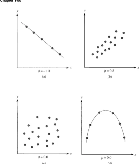
Figure 2.14 graphically illustrates several cases of the correlation coeffi-cient. If the two random variablesXandY are statistically independent, then Corr(X,Y)=Cov(X,Y)=0 (Fig. 2.14c). However, the reverse statement is not necessarily true, as shown in Fig. 2.14d. If the random variables involved are not statistically independent, Eq. (2.70) for computing the variance of the sum of several random variables can be generalized as
Var K k=1 akXk = K k=1 akσk2+2 K−1 k=1 K k=k+1 akakCov(Xk,Xk) (2.50)
Example 2.12 (after Tung and Yen, 2005) Perhaps the assumption of independence
ofPm,Im, andEmin Example 2.11 may not be reasonable in reality. One examines
the historical data closely and finds that correlations exist among the three hydrologic
random variables. Analysis of data reveals that Corr(Pm,Im)=0.8, Corr(Pm,Em)=
−0.4, and Corr(Im,Em)= −0.3. Recalculate the standard deviation associated with
(b) (a) (d) (c) r = –1.0 r = 0.8 r = 0.0 r = 0.0 y x x x x y y y
Figure 2.14 Different cases of correlation between two random variables: (a) perfectly linearly correlated in opposite directions; (b) strongly linearly correlated in a positive direction; (c) uncorrelated in linear fashion; (d) per-fectly correlated in nonlinear fashion but uncorrelated linearly.
Solution By Eq. (2.50), the variance of the reservoir storage volume at the end of the month can be calculated as
Var(Sm+1) =ar(Pm)+Var(Im)+Var(Em)+2 Cov(Pm,Im)
−2 Cov(Pm,Em)−2 Cov(Im,Em)
=Var(Pm)+Var(Im)+Var(Em)+2 Corr(Pm,Im)σ(Pm)σ(Im)
−2Corr(Pm,Em)σ(Pm)σ(Em)−2 Corr(Im,Em)σ(Im)σ(Em)
=(500)2+(2000)2+(1000)2+2(0.8)(500)(2000)
−2(−0.4)(500)(1000)−2(−0.3)(2000)(1000)
The corresponding standard deviation of the end-of-month storage volume is
σ(Sm+1)=
√
8.45×1000=2910 m3
In this case, consideration of correlation increases the standard deviation by 27 percent compared with the uncorrelated case in Example 2.11.
Example 2.13 Referring to Example 2.7, compute correlation coefficient betweenX
andY.
Solution Referring to Eqs. (2.47) and (2.48), computation of the correlation coefficient
requires the determination ofµx,µy,σx, andσyfrom the marginal PDFs ofXandY:
fx(x)=4+3x 2
16 for 0≤x≤2 fy(y)=
4+3y2
16 for 0≤y≤2
as well asE(X Y) from their joint PDF obtained earlier:
fx,y(x,y)=
3(x2+y2)
32 for 0≤x,y≤2
From the marginal PDFs, the first two moments ofX andY about the origin can be
obtained easily as µx=E(X)= 2 0 x fx(x)dx=54=E(Y)=µy E(X2)= 2 0 x2fx(x)dx=2815=E(Y2)
Hence the variances ofX andY can be calculated as
Var(X)=E(X2)−(µx)2=73/240=Var(Y)
To calculate Cov(X,Y), one could first computeE(X Y) from the joint PDF as
E(X Y)= 2 0 2 0 xy fx,y(x,y)dx dy=32
Then the covariance ofX andY, according to Eq. (2.48), is
Cov(X,Y)=E(X Y)−µxµy= −1/16
The correlation betweenX andY can be obtained as
Corr(X,Y)=ρx,y= −1/16
73/240= −0.205
2.5 Discrete Univariate Probability Distributions
In the reliability analysis of hydrosystems engineering problems, several proba-bility distributions are used frequently. Based on the nature of the random vari-able, probability distributions are classified into discrete and continuous types. In this section, two discrete distributions, namely, the binomial distribution and the Poisson distribution, that are used commonly in hydrosystems reliability analysis, are described. Section 2.6 describes several frequently used univari-ate continuous distributions. For the distributions discussed in this chapter and others not included herein, their relationships are shown in Fig. 2.15.
t -∞< x <∞ n Rayleigh 0 x b > min(X1,◊◊◊,XK) X 1 1/X 1 0 = = a a a = b = 1 a = 0 b = 1 a + (b − a)X 2 1 X X --blogX n = 1 a= 1 a 1 X 2 X X 2 1 n n → ∞ 2 = b n=2 2 1/2 n a a = = 2 2 2 1/X X 1 1/n X 2 2/n X 2 X 1 n= a + aX 1 = a n→ ∞ a = n 2 1 1 X X X + m = ab s2 ab2 m + sX a → ∞ = X m s -Standard normal ∞ < < -∞ x Gamma b a, 0 > x Erlang n x , 0 b > Exponential 0 x b > Standarduniform 1 0<x< F 0 x> Weibull b a, 0 > x –1Triangular<x<1 Uniform a < x < b a, b log Y Lognormal y > 0 Beta 0 < x < 1 a, b a = b → ∞ Normal -∞< x <∞ m, s Cauchy a , a x<∞ < -∞ Chi-square n Standard cauchy ∞ < < -∞ x Y =eX x>0 Poisson x = 0,1⋅⋅⋅ v Continuous distributions Discrete distributions 3 1 n n p = Hypergeometric x = 0,1⋅⋅⋅ , min(n1, n2) n1, n2, n3 n = 1 Bernoulli x = 0,1 p n ∞ v = np X1+ ⋅⋅⋅ + XK X1+ ⋅⋅⋅ + XK X1+ ⋅⋅⋅ + XK X1+ ⋅⋅⋅ + XK X1 + ⋅⋅⋅ + XK X1 + ⋅⋅⋅ + XK X1+ ⋅⋅⋅ + XK ← n3 ← ∞ Binomial x = 0,1⋅⋅⋅ n n, p m = np s2 = np(1 – p) n ∞ s2 = v m = v ← X n1, n2
Computations of probability and quantiles for the great majority of the dis-tribution functions described in Secs. 2.5 and 2.6 are available in Microsoft Excel.
2.5.1 Binomial distribution
Thebinomial distributionis applicable to random processes with only two types of outcomes. The state of components or subsystems in many hydrosystems can be classified as either functioning or failed, which is a typical example of a binary outcome. Consider an experiment involving a total of n independent trials with each trial having two possible outcomes, say, success or failure. In each trial, if the probability of having a successful outcome isp, the probability of havingxsuccesses inntrials can be computed as
px(x)=Cn,xpxqn−x forx=0, 1, 2,. . .,n (2.51) whereCn,x is the binomial coefficient, andq=1−p, the probability of having a failure in each trial. Computationally, it is convenient to use the following recursive formula for evaluating the binomial PMF (Drane et al., 1993):
px(x|n,p)= n+1−x x p q px(x−1|n,p)=RB(x)px(x−1|n,p) (2.52) for x=0, 1, 2,. . .,n, with the initial probability px(x=0|n,p)=qn. A simple recursive scheme for computing the binomial cumulative probability is given by Tietjen (1994).
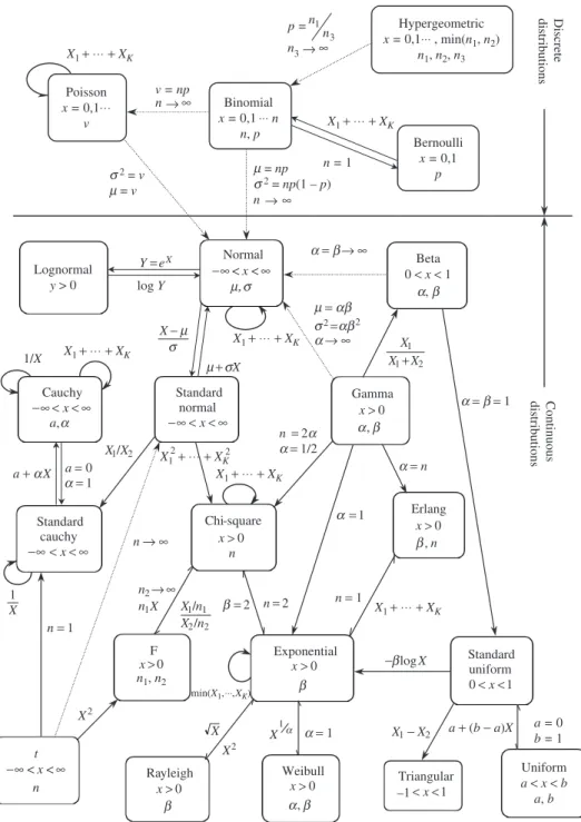
A random variableX having a binomial distribution with parametersnand phas the expectationE(X)=npand variance Var(X)=npq. Shape of the PMF of a binomial random variable depends on the values ofpandq. The skewness coefficient of a binomial random variable is (q− p)/√npq. Hence the PMF is positively skewed if p<q, symmetric if p=q=0.5, and negatively skewed if p>q. Plots of binomial PMFs for different values ofpwith a fixednare shown in Fig. 2.16. Referring to Fig. 2.15, the sum of several independent binomial random variables, each with a common parameter pand differentnks, is still a binomial random variable with parameters pandknk.
Example 2.14 A roadway-crossing structure, such as a bridge or a box or pipe cul-vert, is designed to pass a flood with a return period of 50 years. In other words, the annual probability that the roadway-crossing structure would be overtopped is
a 1-in-50 chance or 1/50=0.02. What is the probability that the structure would be
overtopped over an expected service life of 100 years?
Solution In this example, the random variableX is the number of times the roadway-crossing structure will be overtopped over a 100-year period. One can treat each year as an independent trial from which the roadway structure could be overtopped or not overtopped. Since the outcome of each “trial” is binary, the binomial distribution is applicable.
(a) n=10 p = 0.1 0 0.1 0.2 0.3 0.4 0.5 0 1 2 3 4 5 6 7 8 9 10 x px ( x ) px ( x ) px ( x ) (b) n=10 p = 0.5 0.00 0.05 0.10 0.15 0.20 0.25 0.30 0 1 2 3 4 5 6 7 8 9 10 x (c) n=10 p = 0.9 0 0.1 0.2 0.3 0.4 0.5 0 1 2 3 4 5 6 7 8 9 10 x
Figure 2.16 Probability mass functions of binomial random variables with different values ofp.
The event of interest is the overtopping of the roadway structure. The probability of such an event occurring in each trial (namely, each year), is 0.02. A period of 100 years represents 100 trials. Hence, in the binomial distribution model, the parameters are
p=0.02 andn=100. The probability that overtopping occurs in a period of 100 years
can be calculated, according to Eq. (2.51), as
P(overtopping occurs in an 100-year period)
=P(overtopping occurs at least once in an 100-year period)
=P(X ≥1|n=100,p=0.02) = 100 x=1 px(x)= 100 x=1 C100,x(0.02)x(0.98)100−x