Accepted Manuscript
The Rank Pricing Problem: models and branch-and-cut algorithms
Herminia I. Calvete, Concepci ´on Dom´ınguez, Carmen Gal ´e, Martine Labb ´e, Alfredo Mar´ın
PII: S0305-0548(18)30321-6
DOI: https://doi.org/10.1016/j.cor.2018.12.011
Reference: CAOR 4610
To appear in: Computers and Operations Research
Received date: 3 December 2018
Accepted date: 12 December 2018
Please cite this article as: Herminia I. Calvete, Concepci ´on Dom´ınguez, Carmen Gal ´e, Martine Labb ´e, Alfredo Mar´ın, The Rank Pricing Problem: models and branch-and-cut algorithms, Computers and Operations Research(2018), doi:https://doi.org/10.1016/j.cor.2018.12.011
This is a PDF file of an unedited manuscript that has been accepted for publication. As a service to our customers we are providing this early version of the manuscript. The manuscript will undergo copyediting, typesetting, and review of the resulting proof before it is published in its final form. Please note that during the production process errors may be discovered which could affect the content, and all legal disclaimers that apply to the journal pertain.
ACCEPTED MANUSCRIPT
The Rank Pricing Problem: models and
branch-and-cut algorithms
Herminia I. Calvete
1Concepci´on Dom´ınguez
2,3,4Carmen Gal´e
1Martine Labb´e
2,3Alfredo Mar´ın
41 Universidad de Zaragoza, IUMA, Spain 2 Universit´e Libre de Bruxelles, Belgium
3 Inria Lille-Nord Europe, France 4 Universidad de Murcia, Spain
December 13, 2018
Abstract
One of the main concerns in management and economic planning is to sell the right product to the right customer for the right price. Companies in retail and manufacturing employ pricing strategies to maximize their revenues. The Rank Pricing Problem considers a unit-demand model with unlimited supply and uniform budgets in which customers have a rank-buying behavior. Under these assumptions, the problem is first analyzed from the perspective of bilevel pricing models and formulated as a non linear bilevel program with multiple independent followers. We also present a direct non linear single level formulation bearing in mind the aim of the problem. Two different linearizations of the models are carried out and two families of valid inequalities are obtained which, embedded in the formulations by implementing a branch-and-cut algorithm, allow us to tighten the upper bound given by the linear relaxation of the models. We also study the polyhedral structure of the models, taking advantage of the fact that a subset of their constraints constitutes a special case of the Set Packing Problem, and characterize all the clique facets. Besides, we develop a preprocessing procedure to reduce the size of the instances. Finally, we show the efficiency of the formulations, the branch-and-cut algorithms and the preprocessing through extensive computational experiments.
Keywords: Bilevel Programming, Rank Pricing Problem, Set Packing, Integer Pro-gramming
1
Introduction
The broad development of information and communication technologies produced over the last few decades has resulted in extensive changes in society. In particular, the data availability on customers’ choice behavior has been a key factor in the increasing devel-opment of pricing strategies which also address customers’ preferences. In this context, the use of revenue management strategies, traditionally attributed to airlines and hotel companies, has extended to retail and manufacturing ones ([9], [22]). Generally speaking,
ACCEPTED MANUSCRIPT
pricing optimization problems aim at determining the prices of a series of products in order to maximize the revenue of a company. Setting a low price can lead to a loss of income if customers were willing to pay a higher price, but it can also make a product available to a greater amount of customers. On the contrary, a high price can generate greater revenue, but customers may not purchase it if it is too high. Therefore, a pricing problem is formulated as a bilevel program, in other words, has a hierarchical structure. Thus, its upper level optimization problem consists in maximizing the profit of the com-pany, and part of the constraints force the solution to be optimal to another optimization problem designed to satisfy the customers’ choice rule. For the interested reader, the ref-erences recently collected by Dempe in [7] provide an idea of how fruitful and promising bilevel programming is, and Labb´e and Violin [15] present a review along with models and solution methods for pricing optimization problems that can be modeled as bilevel programs.Pricing problems have attracted wide attention in the literature. We focus on the well-known unit-demand pricing problem, in which each customer is willing to buy at most one product amongst several ones offered by the company, assuming an unlimited supply of each product. Unit-demand models fit multiple sectors where typically customers are only interested in purchasing one product, such as the automotive sector or companies selling electronic devices and electrical appliances (washing machines, vacuum cleaners,
et cetera). In these settings, companies offer the same product with different character-istics and customers base their purchase on a selection rule that takes into account their preferences.
Regarding modelling customer’s purchasing behavior, Shioda et al. [21] provide a re-view of different models in a reservation price framework. In this approach, each customer has a reservation price for each product which reflects how much he is willing to spend on it. Once the pricing strategy is known, the customer will purchase the product with the largest utility, that is, the largest difference between his reservation price for it and the final price of the product. Therefore, the customers’ product choice is entirely based on reservation prices and aims at maximizing their utility. In the case of a limited supply of products, Guruswami et al. [10] study the problem of pricing to maximize the revenue while being envy-free regarding the customers’ valuation for each product. In the limited-supply setting, the envy-freeness is a fairness criterion which guarantees that customers always purchase the product that maximizes their utility among the ones they can afford. When there is unlimited supply, the company can always serve customers and therefore they purchase according to their selection rule, so any pricing is envy-free. Fernandes et al. [8] provide a state-of-art of the envy-free pricing problem. In general, the focus is on the complexity analysis of the problem in order to develop approximation algorithms with logarithmic order, as well as polynomial or pseudo-polynomial time algorithms for interesting special cases which include additional assumptions. Shioda et al. [20] formu-late mixed-integer programming problems to compare the optimal pricing strategies under several probabilistic choice models. Chen et al. [6] provide a state-of-art focused on the computational aspects of the unit-demand pricing model in which the buyer’s valuations of products are characterized by a probability distribution. Heilporn et al. [13] discuss the relationship between the problems of pricing a network or a product line, with the objec-tive of maximizing the revenue and always in the context of utility-maximizing customers. Taking into account the structure of the underlying mixed integer programming
formula-ACCEPTED MANUSCRIPT
tion, Myklebust et al. [16] propose efficient heuristic algorithms for unit-demand pricing problems in which customer budgets and preferences are considered through reservation prices.Rusmevichientong et al. [19] address models based on data collected through an Auto Choice Advisor website. This website collected information on each customer’s require-ments and budget and recommended a ranked list of vehicles according to them. Thus, in the paper each customer is characterized by an ordered list of products and a bud-get. That means that the list of products is sorted according to the degree to which each product fulfills the requirements of the customers. The purchasing decision of a customer is determined by a choice function verifying a certain number of assumptions. Two choice functions of practical interest are analyzed. According to Min-Pricing model, the customer chooses the cheapest product from his list that meets the budget constraints without taking into account the order. If a Rank-Pricing model is assumed, the customer will buy a product under his budget if and only if the products with a higher rank in the customer list are not affordable to him. Briest and Krysta [2] analyze the hardness of ap-proximation of a great variety of unit-demand pricing models under different assumptions on the selection rules, the capacity of the supply and the prices of the products. In addi-tion to rank-buying and min-buying models, these authors consider max-buying models in which the customer buys the product affordable with highest price. In the context of the envy-free pricing problem, Briest [1] considers the unit-demand min-buying pricing problem on the special uniform-budget case, i.e. every customer has the same budget for all the products, which are available in unlimited supply.
In a different but related research field, Discrete Location, we also find customers whose purchase decision is based on preferences. Hanjoul and Peeters [11] study the Simple (or Uncapacitated) Plant Location Problem with Order, in which they assume that a firm wants to select the number and places of a series of facilities to open so as to maximize the revenue, and the clients to be allocated have a preference order on the list of potential sites. Hansen et al. [12] and C´anovas et al. [4] build up on the problem presented in [11], the first ones deriving formulations from the bilevel perspective and the second ones introducing some valid inequalities as well as a very effective preprocessing, along with a computational study to show the efficiency of their approach. Hemmati and Smith [14] relate multi-product pricing, facility location and bilevel optimization. These authors propose a mixed-integer bilevel programming approach for a competitive prioritized set covering problem. This model can be applied to the introduction of new products in a competitive market and to the competitive facility location problem. In both cases each customer has an ordered product (facility) preference list which represents the relative utility of each product (facility).
In this work, we focus on the unit-demand rank pricing model with unlimited supply and uniform-budget. We call this problem the Rank Pricing Problem (RPP) and, to the best of our knowledge, no exact models have been proposed in the literature to deal with it so far. To address the RPP, we present a non linear bilevel formulation in which the company acts as a leader and determines the prices of the products. Once the prices are fixed, each customer, which acts as a follower, solves his own optimization problem. Besides, a non-linear single level formulation is proposed, based on the fact that a customer will purchase the highest-ranked product among all the products he can afford. We linearize the formulations by means of two types of auxiliary variables and derive new valid
ACCEPTED MANUSCRIPT
inequalities. These inequalities are separated and included into the models through the development of a branch-and-cut algorithm. We also take advantage of the fact that some of its constraints constitute a special case of the Set Packing Problem and other properties of the problem in order to strengthen the formulations. We develop some preprocessing techniques to be applied to the instances before solving them. Finally, we present the results of our computational analysis, in which we compare the formulations and show that the results obtained reduce the computational effort when obtaining optimal solutions.The remainder of the paper is organized as follows. Section 2 is devoted to a bilevel formulation for the RPP; in Section 3, the RPP is formulated directly as a single level non linear model; Section 4 includes two linearizations that apply to both models and the development of other valid inequalities to strengthen their linear relaxations through the implementation of branch-and-cut algorithms; in Section 5 some families of clique inequalities associated to a subset of constraints are studied attending to the formula-tions; Section 6 includes some preprocessing results; Section 7 is devoted to testing the performance of the models by means of a computational study; and Section 8 constitutes a conclusion of the paper.
2
Bilevel formulation
LetK ={1, . . . ,|K|}denote the set of customers and I ={1, . . . ,|I|}the set of products. Each customer k ∈ K is represented by a positive budget, a subset of products Sk ⊆ I
he is interested in and a preference value sk
i ∈I for each product i of this subset,i∈Sk,
wheresk
i > skj if customerk prefers productiover productj. We will also assume that for
each customer all preferences are strict, so that he never likes two products the same. As budgets can be equal for different customers, let B ={b1, . . . , bM},M ≤ |K|, denote the
set of different budgets, where b1 < b2 < · · · < bM. To describe the budget of customer
k, we define a functionσ :K → {1, . . . , M}such that σ(k) =` if the budget of customer k is b`. We will say that a customer k1 is richer than k2 if σ(k1)> σ(k2), and the richest
customers will be those whose budget is bM. Without loss of generality, we assume that
customers are interested in at least one product from the company, i.e., Sk 6=∅ ∀k ∈K,
and that each product is included in the list of preference of at least one customer, that is, for any product i ∈ I there exists k ∈ K such that i ∈ Sk. Otherwise, the customer
and/or the product can be removed from the optimization process. Since it will be useful in following sections, we will set b0 = 0.
The RPP aims at establishing the prices of a set of products sold by a company so as to maximize its revenue, the sum of the prices of all items sold. Each customer purchases his most preferred product among the ones he can afford. Note that if a customer cannot afford any product, he will not purchase anything. Therefore, the company, acting as the upper level decision maker, decides on the prices of the products, pi ≥ 0, i ∈ I. At the
lower level of the hierarchy, the customers decide which product to purchase. For this purpose, we introduce binary variables xk
i, k ∈ K, i∈ Sk, for every customer’s purchase
decision, that is,xk
i = 1 if and only if customer k buys producti. The bilevel formulation
ACCEPTED MANUSCRIPT
(BNLp) max p X k∈K X i∈Sk pixki (1a) s.t. pi ≥0, ∀i∈I, (1b)where ∀k ∈K,xk is an optimal solution of
max xk X i∈Sk skixki (1c) s.t. X i∈Sk xki ≤1 (1d) X i∈Sk pixki ≤bσ(k) (1e) xki ∈ {0,1}, ∀i∈Sk, (1f) where constraint (1d) forces customer k to buy one product or none and (1e) establishes that customerk will only buy a product if he can afford it. (BNLp) is a non linear bilevel
problem with multiple independent followers ([3]). Notice that the unlimited supply assumption guarantees that each customer solves a problem involving only the upper level variables and his own variables, thus they are independent followers.
Furthemore, in bilevel programs, the existence of unique solution to the lower level problem is a fundamental assumption to have a well-posed problem. The following result proves that the BNLp is well-posed.
Proposition 2.1. The lower level optimization problems of formulation (BNLp) have a
unique optimal solution.
Proof. The objective function of the lower level problem of (BNLp) for a given customer
k is Pi∈Sksikxki, with coefficients ski ≥ 0, ski 6= skj ∀i, j ∈ Sk, i 6= j. Constraints (1d) ensure that at most one x-variable can take value one. If pi > bσ(k) ∀i ∈ Sk, then the
optimal solution is given by xk
i = 0 ∀i ∈ Sk. Otherwise, the optimal solution is xki = 1
for the unique product i such that sk
i = max
sk
j :j ∈Sk, pj ≤bσ(k) , xkj = 0 for all
j ∈Sk :j 6=i.
It is worth noticing that, although we have focused on the unit-demand case, this formulation and the following ones also apply if a customer k is interested in purchasing ckcopies of the same product and his budget represents the maximum amount he is willing
to pay per copy. Indeed, without loss of generality, it suffices to replace the customer with ck customers with such budget and the same list of preferences. Alternatively, we can
replace the objective function by Pk∈KckP
i∈Skpixki.
The following illustrative example facilitates the understanding of the RPP.
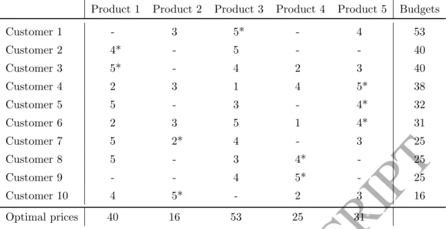
Example 2.2. Table 1 shows the preference matrix and the vector of budgets of an instance of the RPP with 10 customers and 5 products. If product iis the most preferred product for customer k, then sk
ACCEPTED MANUSCRIPT
Product 1 Product 2 Product 3 Product 4 Product 5 BudgetsCustomer 1 -* 3* 5* -* 4* 53 Customer 2 4* -* 5* -* -* 40 Customer 3 5* -* 4* 2* 3* 40 Customer 4 2* 3* 1* 4* 5* 38 Customer 5 5* -* 3* -* 4* 32 Customer 6 2* 3* 5* 1* 4* 31 Customer 7 5* 2* 4* -* 3* 25 Customer 8 5* -* 3* 4* -* 25 Customer 9 -* -* 4* 5* -* 25 Customer 10 4* 5* -* 2* 3* 16 Optimal prices 40* 16* 53* 25* 31*
Table 1: Preference matrix, vector of budgets and an optimal solution to an instance of the RPP with 10 customers and 5 products
k, sk
j = 4, et cetera. In this example, M = 7 and b1 = 16, b2 = 25, b3 = 31, . . ., b7 = 53.
Furthermore, for instance, for customer k = 7, S7 ={1,2,3,5}, and σ(7) = 2 because he
has the second lowest budget. After solving this RPP, we obtain that an optimal solution is provided setting the prices indicated in the last row of Table 1. Taking into account these prices and the preferences, the customers purchase the product whose preference is marked with an asterisk in the preference matrix. For instance, customer 4 can only afford products 2, 4 and 5, and he purchases product 5 (for less than his budget) because it is his preferred one among them; whereas customer 7 purchases product 2, his least preferred one, because it is the only one in his list of preferences that he can afford.
The fact, already observed by Rusmevichientong et al. in [19], that an optimal solution of (BNLp) exists such that p
i ∈B ∀i ∈I, suggests us to define new binary variables vi`,
i ∈ I, ` ∈ {1, . . . , M} representing the prices of products, that is, v`
i = 1 if and only if
product i has price b`. Since each producti has only one price, only one binary variable
v`
i can take value 1 in a feasible solution ∀i∈I. Therefore, the price of product i can be
expressed as pi =PM`=1b`vi`.
We can now reformulate the problem replacing pi variables by v`i variables, replacing
constraints (1b) with the following constraints in order to ensure products have at most one price: M X `=1 v`i ≤1, ∀i∈I, (2a) vi`∈ {0,1}, ∀i∈I, `∈ {1, . . . , M}. (2b)
ACCEPTED MANUSCRIPT
and replacing constraints (1e) of the lower level problem withxki ≤
σ(k)
X
`=1
vi`, ∀k ∈K, i∈Sk. (2c)
We call this bilevel formulation with v-variables (BNLv).
Besides, the fact that the matrix corresponding to the feasible set of each lower level problem of (BNLv) is totally unimodular enables us to relax the integrality constraints
(1f), according to [23, Propositions 3.2 and 3.3]. The lower level problems can be further simplified taking into account that once the leader variables v`
i are known, a subset of
variables is determined. If we consider the subset I(k) = {i ∈ Sk : P`σ=1(k)vi` = 1},
variables{xk
i, k∈K, i∈Sk\I(k)}are automatically settled to 0 since customerk cannot
afford to buy these products. Hence, constraints (2c) can be eliminated and the lower level problem can be formulated as
max xk X i∈I(k) skixki s.t. X i∈I(k) xki ≤1 xki ≥0, i∈I(k).
For each customer k, the dual problem of the lower level problem is min
uk u
k
s.t. uk ≥ski, i∈I(k) uk ≥0.
By duality theory, xk and uk are optimal solutions to the primal and dual problems,
respectively, if and only if
X i∈I(k) skixki =uk X i∈I(k) xki ≤1 uk ≥ski ∀i∈I(k) xk i, uk ≥0.
ACCEPTED MANUSCRIPT
Thus, the resultant formulation after substitution of uk is(BNL) max v,x X k∈K X i∈Sk σ(k) X `=1 b`v` i xk i (3a) s.t. M X `=1 v`i ≤1, ∀i∈I (3b) X i∈Sk xki ≤1, ∀k ∈K (3c) xki ≤ σ(k) X `=1 vi`, ∀k ∈K, i∈Sk (3d) X j∈Sk skjxkj ≥ski σ(k) X `=1 v`i, ∀k∈K, i ∈Sk (3e) vi`, xki ∈ {0,1}, ∀k∈K, i∈Sk, `∈ {1, . . . , M}, (3f) where the objective function (3a) is the same as in model (BNLv) after replacing p
i by
Pσ(k)
`=1 b`vi` (since for vi` = 1 with ` > σ(k), xki = 0). Constraints (3b) are the upper level
constraints (2a) that guarantee that products have at most one price. Constraints (3c) and (3d) are the lower level constraints (1d) and (2c), respectively. These constraints ensure that customers purchase at most one product which they can afford. Finally, constraints (3e) assure that, if customer k can afford product i, he will purchase a productj he likes the same or better than i.
Note that constraints (3e) affect i ∈ Sk instead of i ∈ I(k). If i ∈ Sk\I(k) then
Pσ(k)
`=1 v`i = 0 and the constraint always holds. Otherwise,
Pσ(k)
`=1 vi` = 1 and the constraint
applies.
3
Single level formulation
In this section, we formulate the problem directly as a single level optimization problem. First of all, we introduce some definitionsbased on the ones given by C´anovas et al. ([4]) for the plant location problem with order.
Definition 3.1. Letk ∈K be a customer andi, j ∈Sk two products. It is said that i is
k-better than j if customer k prefers product i over product j, and it is denoted i >k j.
The set of products k-better than i is denoted byB(k, i) = {j ∈Sk:j > k i}.
Definition 3.2. Letk ∈K be a customer andi, j ∈Sk two products. It is said that i is
k-worse than j if customer k prefers product j over product i, and it is denoted i <k j.
The set of products k-worse than i is denoted by B(k, i) = {j ∈Sk:j <k i}.
Since preferences are strict, for any given productsi, j ∈Sk, it followsi >
k j ori <kj.
ACCEPTED MANUSCRIPT
below the customer budget and all the products more preferred thanihave a price higher than his budget. In terms of the binary variables xki,v`i previously defined: xki = 1 ⇔ σ(k) X `=1 vi` = 1 and σ(k) X `=1 v`j = 0 ∀j ∈B(k, i).
Using this notation and decision variables xk
i, vi`, a single level non linear formulation
is (SLNL) max v,x X k∈K X i∈Sk σ(k) X `=1 b`vi` xki (4a) s.t. X i∈Sk xki ≤1, ∀k ∈K (4b) M X `=1 vi`≤1, ∀i∈I (4c) xki + σ(k) X `=1 vj` ≤1, ∀k ∈K, i∈Sk, j ∈B(k, i) (4d) xki + M X `=σ(k)+1 vi` ≤1, ∀k ∈K, i ∈Sk (4e) v` i, xki ∈ {0,1}, ∀k ∈K, i ∈Sk, `∈ {1, . . . , M}, (4f)
where constraints (3d) have been replaced by (4e) using constraints (4c). Constraints (4d), also called preference constraints, are given by the previous reasoning and can be strengthened by means of the following result:
Proposition 3.3. The following constraints
X j∈B(k,i) xkj + σ(k) X `=1 vi` ≤1, ∀k ∈K, i∈Sk:B(k, i)6=∅, (5)
are valid for (SLNL) and dominate constraints (4d).
Proof. First of all, we shall prove the validity of (5). We havePj∈B(k,i)xk j ≤ P j∈Ixkj ≤1 using (4b) and Pσ`=1(k)v` i ≤ PM
`=1v`i ≤ 1 because of (4c). Furthermore, provided that
product i is within k’s budget, i.e., if Pσ`=1(k)v`
i = 1, then customer k will not buy any
product k-worse for him than i, so Pj∈B(k,i)xk
j = 0, so (5) are valid.
If we change the notation of (5) and write Pi0∈B(k,j)xki0 +P`σ=1(k)vj` ≤ 1, ∀k ∈ K,
j ∈Sk :B(k, j)6=∅, and taking into account that when j is k-better than i∈ Sk then i
ACCEPTED MANUSCRIPT
xki + σ(k) X `=1 vj` ≤ X i0∈B(k,j) xki0 + σ(k) X `=1 vj` ≤1.Therefore, we have proved that (5) are stronger than (4d).
4
Linearizing and strengthening formulations
Formulations (BNL) and (SLNL) are non linear because of the objective functions (3a) and (4a). Since both objective functions are the same, from now on we refer to (4a). In order to linearize it, one approach consists in introducing variableszk,k ∈K, representing
the profit obtained from customer k. Thus, the objective (4a) can be replaced by max
v,x,z
X
k∈K
zk
and the following constraints need to be added to the formulation
zk ≤ σ(k) X `=1 b`vi`+bσ(k) 1−xki, ∀k ∈K, i∈Sk (6a) zk ≤bσ(k)X i∈Sk xki, ∀k ∈K, (6b)
where constraints (6a) ensure that if customer k buys producti,zk=Pσ(k)
`=1 b`vi` and (6b)
guarantee zk ≤ 0 if customer k does not make any purchase. Constraints (6a) can be
strengthened taking into account that customer k buys at most one item, obtaining zk≤ σ(k) X `=1 b`vi`+bσ(k) X j∈Sk:j6=i xkj, ∀k ∈K, i∈Sk. (7)
Therefore, we can reformulate problem (SLNL) obtaining a linear model as follows: (SLL1) max v,x,z X k∈K zk (8a) s.t. X i∈Sk xki ≤1, ∀k∈K (8b) M X `=1 vi` ≤1, ∀i∈I (8c) X j∈B(k,i) xkj + σ(k) X `=1 v`i ≤1, ∀k ∈K, i∈Sk: B(k, i)6=∅ (8d) xk i + M X `=σ(k)+1 v` i ≤1, ∀k ∈K, i∈Sk (8e)
ACCEPTED MANUSCRIPT
zk≤ σ(k) X `=1 b`vi`+bσ(k) X j∈Sk:j6=i xkj, ∀k ∈K, i∈Sk (8f) zk≤bσ(k)X i∈Sk xki, ∀k ∈K (8g) vi`, xki ∈ {0,1}, zk ≥0 ∀k ∈K, i∈Sk, `∈ {1, . . . , M}. (8h) The nonlinearity of the objective function (4a) can also be handled through the intro-duction of variables zki, k ∈K, i ∈Sk, representing the profit obtained from customer k
associated to product i. With these variables, the objective is
max v,x,z X k∈K X i∈Sk zik
and the following constraints ought to be added to the model:
zik≤ σ(k) X `=1 b`vi`, ∀k ∈K, i∈Sk zik≤bσ(k)xki, ∀k ∈K, i∈Sk.
Thus, the resulting model is
(SLL2) max v,x,z X k∈K X i∈Sk zk i (9a) s.t. X i∈Sk xki ≤1, ∀k∈K (9b) M X `=1 vi` ≤1, ∀i∈I (9c) X j∈B(k,i) xkj + σ(k) X `=1 v`i ≤1, ∀k ∈K, i∈Sk: B(k, i)6=∅ (9d) xki + M X `=σ(k)+1 vi` ≤1, ∀k ∈K, i∈Sk (9e) zik≤ σ(k) X `=1 b`vi`, ∀k ∈K, i∈Sk (9f) zik≤bσ(k)xki, ∀k ∈K, i∈Sk (9g) vi`, xki ∈ {0,1}, zki ≥0 ∀k ∈K, i∈Sk, `∈ {1, . . . , M}. (9h)
In the formulations (SLL1) and (SLL2), the values of thez-variables associated to an
assignment of prices to products (v-variables) and products to customers (x-variables) are obtained, respectively, by means of constraints (8f)-(8g) and (9f)-(9g). Although
ACCEPTED MANUSCRIPT
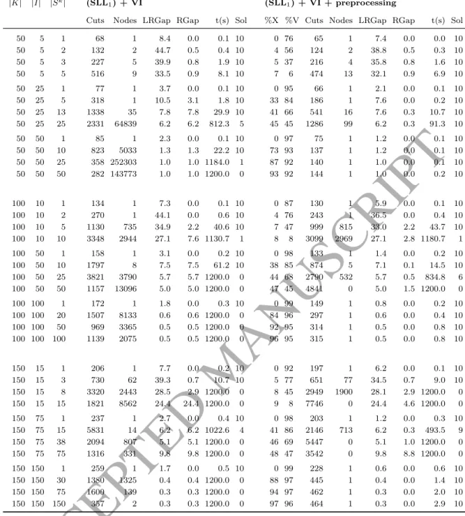
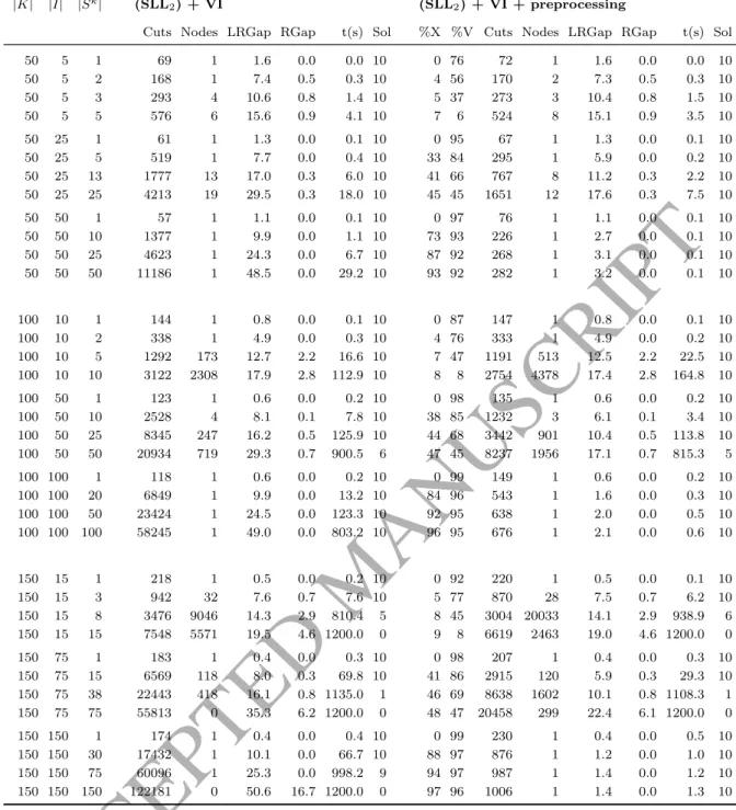
these constraints suffice to obtain the desired values of the z-variables, they lead to weak linear relaxations. Given the shape of the objective function, this weakness is directly transmitted to the upper bounds in the branch-and-bound method. Furthermore, in (8f) (resp. (9f)), a bound for z is obtained exclusively from the v-variables, and in (8g) (resp. (9g)), from the x-variables. These two issues invite to develop stronger constraints on the z-variables.In what follows, two families of valid inequalities for (SLL1) and (SLL2) are presented.
As will be shown in the computational study, they produce the desired improvement in the upper bounds given by the LP relaxation, and they have the particularity of relating the z-variables with both the x- and the v-variables at a time.
Proposition 4.1. The following inequalities are valid for (SLL1):
zk ≤ X i∈Sk brkixk i + σ(k) X `=rk i+1 b`−brki v`i + X `∈Qk i b`−brki xki +vi`−1 , (10) ∀k ∈K, integers rk i ∈ {0, . . . , σ(k)} ∀i∈Sk and subsets Qki ⊆ {1, . . . , rki −1} ∀i∈Sk.
Proof. Notice that in the case rk
i = 0, set Qki must be empty. We aim at proving that
constraints (10) are valid for (SLL1). Let us assume xki0 = 1 for some i0 ∈Sk, and prove
that the sum of the addends corresponding to product i0 in the right hand side of the
constraint is greater than or equal to its price. Thus, such sum is
brik0 + σ(k) X `=rk i0+1 b`−brki0 v`i0 + X `∈Qk i0 b`−brki0 vi0` , (11)
and we know that vi0`0 = 1 for some`0 ≤σ(k). If `0 > ri0k, then v`i0 = 0 ∀` ∈ Qki0 and we
get brik0 + (b`0 −brik0) = b`0, which is exactly the price of i
0. On the other hand, if `0 ≤ri0k
we have v`
i0 = 0 ∀` :rki0 < `≤σ(k), and therefore (11) becomes
brki0 + X `∈Qk i0 b`−brk i0 v` i0. If`0 ∈/ Qki0, we obtainb rk
i0, which is greater than or equal tob`0 becauserk
i0 ≥`0; otherwise,
if `0 ∈Qki0, then the term becomes b rk
i0 + (b`0 −br
k
i0) = b`0.
Now, let us suppose xk
i0 = 0 for i0 ∈Sk. Then the addends corresponding to product
i0 become σ(k) X `=rk i0+1 b`−brik0 vi0` + X `∈Qk i0 b`−brik0 vi0` −1. Since (b`−brk i0)>0 for` :rk i0 < `≤σ(k) and (b`−b rk i0)<0 for `∈Qk
i0, then the sum is
greater than or equal to zero. Therefore, if xk
i = 0∀i∈Sk,zk will be bounded from above by a sum of non-negative
ACCEPTED MANUSCRIPT
for a fixed customer k, say xki0, the upper bound will be obtained as the sum of the term
corresponding to product i0, which has been proved to be greater than or equal to the
price assigned to i0, plus some non-negative addends.
Remark 4.2. The family of inequalities (10) contains all of the previous upper bound constraints on zk of (SLL
1). Constraints (8f) are obtained by, given a customer k ∈ K
and a product i∈Sk, setting rk
i = 0, rjk =σ(k) ∀j ∈Sk\ {i}andQkj =∅ ∀j ∈Sk in (10);
constraints (8g), by, given a customer k ∈K, setting rk
i =σ(k) and Qki =∅ ∀i∈Sk. Proposition 4.3. The inequalities of the following family are valid for (SLL2):
zki ≤brikxk i + σ(k) X `=rk i+1 b`−brki vi`+ X `∈Qk i b`−brki xki +v`i −1, (12) ∀k ∈K, i∈Sk, any integer rk
i ∈ {0, . . . , σ(k)} and any subset Qki ⊆ {1, . . . , rik−1}.
Proof. First assume that xk
i = 1. This implies vi`0 = 1 for some `0 ≤ σ(k). If `0 ≤ rik,
then v` i = 0∀` :rik < `≤σ(k) and (12) becomeszik ≤br k i +P `∈Qk i(b `−brk i)v` i. If `0 ∈Qki,
then the right hand side of the constraint is brk
i + (b`0 −brki) = b`0, which is valid as it
is the exact price of product i; otherwise, the right hand side of the constraint is brk i,
valid since brk
i ≥ b`0. If `0 > rk
i, then vi` = 0 ∀` ∈ Qki and the inequality we obtain is
zk i ≤br
k
i + (b`0 −brki), also valid.
On the other hand, if we assume xki = 0, then the inequality holds trivially because
its right hand side is non negative and zk i = 0.
Remark 4.4. The family of inequalities (12) contains all of the previous upper bound constraints on zk
i of (SLL2): constraints (9f) are obtained by setting rki = 0 and Qki = ∅
∀k ∈K, i∈Sk, whereas constraints (9g) appear as a result of setting rk
i =σ(k), Qki =∅
∀k, i∈Sk.
The number of inequalities of Propositions 4.1 and 4.3 increases exponentially as the number of customers and products grows. However, these inequalities can be efficiently separated and added dynamically to formulations (SLL1) and (SLL2), respectively, in a
branch-and-cut mode. Thus, regarding the family of valid inequalities (10), and given a fractional optimal solution of the linear relaxation of (SLL1), (v`i, xki, zk), our aim is to
find, for each k∈K, integersrk
i and subsets Qki ∀i∈Sksuch that the upper bound given
by the right hand side of the resultant constraint of the family is as tight as possible. As the sum given by the right hand side of (10) can be decomposed by products and given that z is fixed, our problem reduces to
min r∈{0,...,σ(k)}, Q⊆{1,...,r−1} brxki + σ(k) X `=r+1 b`−brv`i +X `∈Q b`−br xki +v`i −1, (13)
where (k, i)∈K×Sk is fixed, and we have denotedrk
i asr and Qki as Qso as to simplify
notation. It is worth noticing that this pair (r, Q) also minimizes the right hand side of the corresponding constraint of family (12) when given an optimal fractional solution of
ACCEPTED MANUSCRIPT
the linear relaxation of (SLL2), (v`i, xki, zki), and fixed (k, i) ∈ K ×Sk. Thus, finding apair (r, Q) that minimizes (13) for a given customerk and producti not only leads to the development of an efficient separation algorithm for the set of valid inequalities (10), but also for the set (12).
The fact that (b`−br)≤0∀`≤rimplies that, for a givenr,Qr :={` ∈ {1, . . . , r−1}:
xk
i+v`i >1}minimizes (13). Therefore, ifW(r) is the value of the sum (13) whenQ=Qr,
our problem consists in minimizing W(r) forr ∈ {0, . . . , σ(k)}.
To do so, we shall study the variation of W(r) as r increases. Given that Qr+1 =
Qr∪ {r} if xk
i +vri >1,Qr+1 =Qr otherwise, for r < σ(k) we get
W(r+ 1)−W(r) = br+1xki + σ(k) X `=r+2 b`−br+1v`i + X `∈Qr+1 b`−br+1 xki +v`i −1 − brxki + σ(k) X `=r+1 b`−brv`i +X `∈Qr b`−br xki +v`i −1 = (br+1−br)xki + σ(k) X `=r+2 br−br+1v`i − br+1−brvri+1 + X `∈Qr+1 br−br+1 xki +v`i −1 = br+1−br xki − σ(k) X `=r+1 v`i + X `∈Qr+1 1−xki −v`i . (14)
First of all, we are going to prove that, when r increases from 0 to σ(k), W(r) first decreases and then increases. We can achieve that by proving that W(r)−W(r−1) ≥ 0⇒W(r+ 1)−W(r)≥0. Sincebr+1−br >0∀r < σ(k), it follows from (14) thatW(r+
1)−W(r) ≥ 0⇔ xk i − Pσ(k) `=r+1v`i + P `∈Qr+1 1−xki −v`i ≥0 ∀r < σ(k), and therefore demonstrating the above is equivalent to provingxk
i− Pσ(k) `=r+1v`i+ P `∈Qr+1 1−xki −v`i − xk i − Pσ(k) `=r v`i + P `∈Qr 1−xki −v`i ≥0. But we have xki − σ(k) X `=r+1 v`i + X `∈Qr+1 1−xki −v`i− xki − σ(k) X `=r v`i + X `∈Qr 1−xki −v`i =vri + min0,1−xki −vri = minvri,1−xki ≥0. Hence,W(r) reaches its minimum value for the smallestrsuch thatW(r)−W(r−1)≤
0 and W(r+ 1)−W(r)>0.
Furthermore, noticing in (14) that P`∈Qr+1 1−xki −v`i
≤0 ∀r allows us to deduce that W(r) − W(r − 1) ≤ 0 provided that xk
i −
Pσ(k)
`=r v`i ≤ 0, i.e., if r is such that
xk i ≤
Pσ(k)
`=r v`i. This fact saves us having to compute the whole sum (14) in order to know
if W(r)−W(r−1)≤0 whenever xk i ≤
Pσ(k)
ACCEPTED MANUSCRIPT
After finding a separation for valid inequalities (10), the next step consists in defining a procedure to incorporate these inequalities into formulation (SLL1) dynamically in abranch-and-cut framework where the starting subproblem of every child node is the final formulation of the parent node with the corresponding branchingx- orv-variable fixed to either zero or one. A scheme of this procedure is depicted in Algorithm 1. Preliminary testing shows that the best strategy amounts to adding these inequalities to the formu-lation provided that the node depth in the branching tree is less than or equal to 4. The termination criterion is that the optimal value of the linear relaxation of that node does not improve in the last iteration. Both the algorithm and the branch-and-cut procedure used to include dynamically inequalities (12) into model (SLL2) are analogous to these
ones.
Algorithm 1 Separation of inequalities (10) Let (xk
i, v`i, zk) be an optimal fractional solution of the linear relaxation of (SLL1).
For every customer k∈K do
Step 1. For every producti∈Sk do
Step 1.1. Setrki = 0. Step 1.2. If rk
i < σ(k) and
Pk
`=1v`i ≤xki, update rik :=rik+ 1 and repeat Step
1.2.
Otherwise, go to Step 1.3.
Step 1.3. If rki < σ(k) and W(rik+ 1)−W(rik) ≤ 0, update rik := rik+ 1 and
repeat Step 1.3.
Otherwise, go to Step 2. Step 2. Set Qk
i :={`∈ {1, . . . , rki −1}:xki +v`i >1} ∀i∈Sk.
Step 3. Incorporate constraint
zk≤ X i∈Sk brikxk i + σX(k) `=rk i+1 b`−brki v` i+ X `∈Qk i b`−brki xk i +v`i−1
to the formulation if and only if it is violated.
5
Polyhedral analysis of the set packing subproblem
In this section, we analyze the subproblem of model (SLL1) (resp. model (SLL2))
asso-ciated to x- and v-variables and constraints (8b)-(8e) (resp. constraints (9b)-(9e)), given that it constitutes a special case of a Set Packing Problem (SPP). Since this subproblem is the same for both models (SLL1) and (SLL2), in the rest of the section we shall refer
to the subproblem of model (SLL1).
An SPP is a problem in the form of
max{ct:At≤1w, t∈ {0,1}u},
where c∈Ru, A∈ {0,1}w×u and 1
ACCEPTED MANUSCRIPT
The polyhedral structure of the SPP has been widely studied in the literature. The interested reader is referred to [18], where the basis of this section is presented, and to [5], where further results are presented and the main papers on the topic are referenced. In the following paragraphs we briefly expose the notation and results necessary in the section. For details, the reader may consult [17].Associated with each instance of an SPP, let the intersection graph be G = (V, E), where each node in the set V is associated to a variable of the problem and (vi, vj) ∈E
if and only if aki +akj = 2 in some row of A. The neighborhood of a node v is the
set of nodes adjacent to v. A non empty subset of pairwise non adjacent nodes in G is known as a packing, and the problem of obtaining an optimal solution of an SPP is equivalent to that of obtaining a packing of maximum cardinality on its intersection graph. A complete graph is that in which all the nodes are pairwise adjacent, and a clique in G is a maximal complete subgraph. The incidence vector of a subsetV0 ⊂V is a binary vector (t1, . . . , t|V|) where tj = 1 if and only if the jth node of V belongs to V0,
for j ∈ {1, . . . ,|V|}.
LetP(G) be the convex hull of the incidence vectors of all the packings of the intersec-tion graphG, i.e., the convex hull of all the feasible solutions of SPP. Since facet defining inequalities are not dominated by any other valid inequality, one way of confirming that our formulation (or part of it) is tight consists in proving that its constraints are facet-defining. And, as stated in [18], an inequality in the formPv∈V0xv ≤1, whereV0 ⊂V, is
a facet forP(G) if and only if the subgraph induced by V0 is a clique inG. Clique facets are particularly interesting because they can always provide a valid formulation and their addition to a problem generally provides better results (when trying to solve it) than the addition of other types of facets which are more complex, such as lifted odd holes.
5.1
Set packing subproblem of (SLL
1)
In order to apply the SPP properties to our problem, we begin by identifying the intersec-tion graph GSLL associated to the previously defined subproblem of formulaintersec-tion (SLL1).
The large amount of edges of this graph makes drawing it impractical, so we will follow a different approach in order to describe the intersection graph based on the following proposition.
Proposition 5.1. Given the intersection graphGSLLassociated to the subgraph of(SLL1):
(1) Two nodes xk
i, xkj, i=6 j, are adjacent ∀i, j ∈Sk. (2) Two nodes xk
i, xk
0
i , k 6=k0, are never adjacent. (3) Two nodes xk
i, xk
0
j , k 6= k0, i 6= j, are adjacent if and only if σ(k) ≥ σ(k0) and
j ∈B(k, i) (or, equivalently, i∈B(k, j)).
(4) Two nodes xk
i, v`i, are adjacent if and only if ` > σ(k). (5) Two nodes xk
i, v`j, i6=j are adjacent if and only if `≤σ(k) and j ∈B(k, i). (6) Two nodes v`
i, v`
0
ACCEPTED MANUSCRIPT
(7) Two nodes v` i, v`
0
j , i6=j, are never adjacent.
Proof.
(1) A customer k purchases at most one product.
(2) The fact that a customer k purchases a product i does not imply that another customer cannot afford it (that depends on i’s price), and therefore does not allow us to determine whether another customer is going to buy it or not.
(3) Let us suppose xk
i = 1, i.e., customer k purchases product i. That implies k is not
able to afford any product j that is k-better than i, and therefore no customer k0 with σ(k0)≤σ(k) will be able to afford it either, hence xk0
j = 0. However, the fact
that k purchases product i does not allow us to infer which products will not be purchased by other customersk0 richer that k or which customers will not purchase a productj ∈B(k, i)∪ {i}.
(4) If xk
i = 1, k can afford product i, so there must exist `0 ≤ σ(k) such that vi`0 = 1.
Since product i can have one price at most, it followsv`
i = 0 ∀` > σ(k). (5) Let us suppose xk
i = 1, i.e., customer k purchases product i. That implies k is
not able to afford any product j that is k-better than i, i.e., v`
j = 0 ∀j ∈ B(k, i),
∀` ≤ σ(k). However, it does not provide any insight into the prices of products j ∈B(k, i).
(6) A producti can have at most one price.
(7) Knowing the price of a product does not provide any insight into the price of the rest.
Having identified the intersection graph GSLL, the next subsection focuses on charac-terizing all its cliques.
5.2
Characterization of all the cliques in the intersection graph
We first include a lemma that will be useful when characterizing all the cliques.Lemma 5.2. Any clique inGSLL which contains nodes vi`1, vi`2 with`1 < `2, containsvi`
∀` such that`1 < ` < `2.
Proof. Let (V0, E0) be a clique in GSLL and supposev`1i ,v`2i ∈V0, for`1 < `2.
Let us suppose that there existsk ∈K withxk
i ∈V0. Then, xki is adjacent to vi`1, and
thus for Prop. 5.1(4) it follows σ(k) < `1. Therefore, for every ` > `1 > σ(k), the same
result implies xk
ACCEPTED MANUSCRIPT
Now let us suppose that there exist k ∈ K and j ∈ Sk, j 6= i, with xkj ∈ V0. By
hypothesis we have xk
j adjacent to v`2i , which for Proposition 5.1(5) implies i ∈ B(k, j)
and σ(k)≥ `2. Thus, for every` < `2 ≤ σ(k), it follows from the same result that xkj is
adjacent to v` i.
Finally, we know from Proposition 5.1(6) and (7) that v`
j adjacent to v `1 i ⇔ j = i, hence v` i is adjacent tov` 0 i ∀`6=`0 and vj` ∈/ V0 for j 6=i.
All in all, we have proven that for ` such that`1 < ` < `2, any variablexkj orv`
0
i ∈V0
is adjacent tov`
i. Thus, the statement follows.
Before proving the main results of this section, we introduce some sets that generalize B(k, i).
Definition 5.3. Let k be a customer and P ⊆ Sk a subset of products in which k is
interested. Then we define B(k, P) as the set {i∈Sk : i >
k j ∀j ∈ P} of products that
are preferred bykto all the products inP. SimilarlyB(k, P) :={i∈Sk : i <
k j ∀j ∈P}.
In the special case whenP =∅ we defineB(k,∅) :=I and B(k,∅) :=I.
Now we can state the two main results in this section. Note that, in order to keep a consistent notation, a set{k2, . . . , kn}is defined in Theorem 5.4 that will be extended to
{k1, . . . , kn} in Theorem 5.5.
Theorem 5.4. Given a set of customers {k2, . . . , kn}, n ≥2, with σ(k2) ≤ · · · ≤σ(kn),
and non empty pairwise disjoint sets of products Pkq ⊆Skq, q = 2, . . . , n, such that
Pkq ⊆ q\−1 r=2: σ(kr)<σ(kq) B(kq, Pkr) \ q\−1 r=2: σ(kr)=σ(kq) B(kq, Pkr)∪B(kr, Pkr) ∀q∈ {3, . . . , n},
the following inequalities are valid for (SLL1):
n X q=2 X j∈Pkq xkq j ≤1. (15)
Valid inequalities (15) are facets for the subproblem of (SLL1) if and only if @(k0, i0) ∈
K×Sk0 satisfying 1. i0 ∈B(kq, Pkq) ∀q ∈ {2, . . . , n}: σ(kq)≥σ(k0), 2. i0 ∈B(k0, Pkq) ∀q∈ {2, . . . , n}: σ(kq)≤σ(k0), and | n [ q=2: σ(kq)=σ(k2)
Pkq| ≥ 2. Furthermore, all the clique facets for the subproblem of (SLL
1)
ACCEPTED MANUSCRIPT
Proof. Let GSLL = (VG, EG) be the intersection graph of the subproblem of (SLL1)as-sociated to x- and v-variables and constraints (8b)-(8e), and let Q= (V0, E0) be a clique of GSLL containing only x-variables.
Let k2 be a customer with minimum budget in the clique and a subset of products
Pk2 ⊆Sk2 such that xk2
j ∈V0 ∀j ∈Pk2 (taking into account that, by Proposition 5.1(1),
xk2i is adjacent toxk2j ∀i6=j).
Provided that there exist customers kq, ∀q ∈ {3, . . . , n} such that σ(k2) ≤ σ(k3) ≤
· · · ≤σ(kn) and sets of productsPkq ⊆Skq, Pkq 6=∅ ∀q ∈ {3, . . . , n}, such that xkjq ∈V0
∀j ∈ Pkq, then by Proposition 5.1(2) Pk2, . . . , Pkn are pairwise disjoint, and verify the
following conditions: • Pkq ⊆ q\−1 r=2 σ(kr)<σ(kq) B(kq, Pkr), ∀q∈ {3, . . . , n}.
Otherwise, there exist kr with σ(kr) < σ(kq) and products i ∈ Pkr, j ∈ Pkq such
that xkr
i , x kq
j ∈ V0 but j /∈ B(kq, i), and by Proposition 5.1(3) this implies xkir,
xkq
j are not neighbors in the intersection graph. Therefore, V0 does not induce a
complete graph. • Pkq ⊆ q\−1 r=2 σ(kr)=σ(kq) B(kq, Pkr)∪B(kr, Pkr) , ∀q∈ {3, . . . , n}.
Otherwise, there exist kr with σ(kr) = σ(kq) and products i ∈ Pkr, j ∈ Pkq such
that xkr
i , x kq
j ∈ V0 but Proposition 5.1(3) does not hold for k = kr, k0 = kq or for
k =kq, k0 =kr, and henceV0 does not induce a complete graph.
Therefore, the above conditions guarantee that the nodes corresponding with the x-variables in an inequality in the form of (15) induce a complete graph, so the family of inequalities (15) is valid.
In addition, if there exist (k0, i0)∈K×Sk0 meeting the conditions of the statement,
then xk0i0 is adjacent in the intersection graph to every other node in V0 by Proposition 5.1(3)and conditions 1 and/or 2, and therefore the complete subgraph is not maximal.
On the other hand, if |
n
[
q=2:
σ(kq)=σ(k2)
Pkq| ≥ 2 holds, no v-variable can be adjacent in
the intersection graph to all nodes in V0. Otherwise, Pk2 = {i} and either n = 2 or
σ(k2)< σ(k3), and hence variable viσ(k2)+1 would be adjacent to every node in V0 and the
complete subgraph would not be maximal.
Theorem 5.5. Given a nonempty set L = {`1, . . . , `p} ⊆ {1, . . . , M}, a product i ∈ I
ACCEPTED MANUSCRIPT
• if `1 > 1, a customer k1 such that σ(k1) = `1 −1, i ∈ Sk1, and a set Pk1 = {i};
otherwise, Pk1 =∅;
• if `p < M, customers k2, . . . , kn, n ≥ 2, such that `p = σ(k2) ≤ · · · ≤ σ(kn)
(n = 1 otherwise) and non empty pairwise disjoint sets of products Pkq ⊆Skq\ {i},
q= 2, . . . , n such that Pk2 ⊆B(k 2, i) and Pkq ⊆ q\−1 r=1: σ(kr)<σ(kq) B(kq, Pkr) \ q\−1 r=1: σ(kr)=σ(kq) B(kq, Pkr)∪B(kr, Pkr) ∀q∈ {3, . . . , n},
the following inequalities are valid for (SLL1):
X `∈L vi`+ n X q=1 X j∈Pkq xkq j ≤1. (16)
Valid inequalities (16) are facets for the previously defined subproblem of (SLL1) if and
only if @(k0, i0)∈K×(Sk0 \ {i}): σ(k0)≥`p satisfying
1. i0 ∈B(kq, Pkq) ∀q ∈ {1, . . . , n}: σ(kq)≥σ(k0),
2. i0 ∈B(k0, Pkq) ∀q∈ {1, . . . , n}: σ(kq)≤σ(k0).
Furthermore, all the clique facets for the subproblem of (SLL1) containing v-variables are
in family (16).
Proof. Let GSLL = (VG, EG) be the intersection graph of the previously defined
subprob-lem of (SLL1) and letQ= (V0, E0) be a clique of GSLL containingv-variables. Taking into
account Proposition 5.1(7), all v-variables in the same clique must share the subindex, and by Lemma 5.2, all v-variables in the same clique must have consecutive superindices. We represent with L = {`1, . . . , `p} this set of consecutive superindices and with i the
common subindex. We thus distinguish several cases depending on L: 1. L={1, . . . , M}.
Then by Proposition 5.1(5)we know that a nodexk
j in the neighborhood ofvi1, . . . , viM
must satisfyσ(k) = M and j ∈B(k, i). However, the richest customers always pur-chase their most preferred product, and therefore we have removed all thesex-nodes from the intersection graph, i.e., Pk2 =· · ·=Pkn =∅.
Since Proposition 5.1(4) does not either provide any node adjacent to v`
i ∀`, we
obtain Pk1 =∅and thus the set of nodes {v`
i : `∈ {1, . . . , M}} induces a maximal
ACCEPTED MANUSCRIPT
2. L={`1, . . . , M} for some `1 >1.As v`
i ∈/ V0 ∀` ∈ {1, . . . , `1 −1}, a node adjacent to v`i for ` ≥ `1 but not to vi`1−1
must belong to the clique. Applying Lemma 5.2 and Proposition 5.1, we know this node corresponds with an x-variable, i.e., there exists a node xk
j ∈ V0 for some
customer k and product j. As in the previous case, Proposition 5.1(5) does not provide any node adjacent to vM
i , thus Pk2 = · · · = Pkn = ∅. Therefore, node xkj
must be adjacent to v`
i for ` ≥ `1 by Proposition 5.1(4), so j = i and k =k1 for a
customer k1: σ(k1)< `1 and Pk1 ={i}. Since xk1i is not adjacent to vi`1−1, also by
Proposition 5.1(4) σ(k1)≥`1−1, and hence σ(k1) =`1−1.
If we suppose there exists another node xk
j ∈ V0, then xkj must be adjacent to vi`
∀` ≥ `1 by Proposition 5.1(4), and therefore j = i. However, xki and xk1i are not
adjacent for any customer k 6=k1 by (2), so the set {vi` : ` ≥`1} ∪ {xk1i }induces a
clique in GSLL.
3. L={1, . . . , `p} for some `p < M.
Since v`
i ∈/ V0 ∀` > `p, applying Lemma 5.2 and Proposition 5.1 there must exist a
node xk
i0 ∈V0 such that xki0 is adjacent to v `p
i but not to v `p+1
i . Proposition 5.1(4)
does not provide any node adjacent tov1
i, hence Pk1 =∅andxki0 has to be adjacent
to v`
i, `≤ `p, by Proposition 5.1(5). Hence, there exists a customer k2: σ(k2)≥`p
and a subset of products Pk2 ⊆ B(k
2, i) such that i0 ∈Pk2 and xk2j ∈V0 ∀j ∈Pk2
(taking into account that, by Proposition 5.1(1), xk2j is adjacent to xjk20 ∀j 6= j0). Since xk2i0 is not adjacent to v`p+1
i , it follows σ(k2) = `p.
Provided that there exist customers kq, ∀q ∈ {3, . . . , n} such that σ(k2)≤ σ(k3) ≤
· · · ≤ σ(kn) and sets of products Pkq ⊆ Skq, Pkq 6= ∅ ∀q ∈ {3, . . . , n}, such that
xkq
j ∈ V0 ∀j ∈ Pkq, then by Proposition 5.1(2) Pk1, . . . , Pkn are pairwise disjoint.
Moreover,Pkq ⊆Skq\ {i} ∀q∈ {3, . . . , n}; otherwise, xkq
i ∈V0 for somekq: σ(kq)≥
`p and is not adjacent tovi`p (Proposition 5.1(4)), thusV0does not induce a complete
graph.
Applying arguments analogous to those of Theorem 5.4, the rest of the conditions stated above must hold.
4. L={`1, . . . , `p} for some `1 >1,`p < M.
Applying arguments analogous to those of the previous items, we can conclude that there exist customers k1 ∈ K: σ(k1) = `1 −1, i ∈ Sk1 such that Pk1 = {i} and
k2 ∈ K: σ(k2) = `p with Pk2 ⊆ B(k2, i), Pk2 6=∅. The rest of the conditions also
hold applying a reasoning analogous to that of Theorem 5.4.
Now that we have established the different shapes that clique facets can adopt, we are able to determine whether constraints (8b)-(8e) always define clique facets in the corresponding subproblem of (SLL1). Thus, we can conclude that constraints (8c) and
(8e) always define clique facets by applying cases 1 and 2 of the proof of Theorem 5.5, respectively. By Theorem 5.4, and given thatB(k, Sk) = ∅ ∀k, we know a valid inequality
ACCEPTED MANUSCRIPT
from the family (8b) will be a clique if and only if|Sk| ≥2 and@(k0, i0)∈K×Sk0 satisfying
σ(k0)≥ σ(k) and i0 ∈ B(k0, Sk). As for constraints (8d), they do not necessarily define
clique facets either but, like in the former case, they define clique facets in most cases. Even though the valid inequalities given by Theorems 5.4 and 5.5 are facet defining on the subproblem of (SLL1) associated to x- and v-variables and constraints (8b)-(8e),
they might not define facets on the polyhedra which is obtained once we consider also z-variables and their corresponding constraints of model (SLL1). Nevertheless, they are
still strong valid inequalities and, as such, make the extended formulation (SLL1) stronger
in turn. As we have previously stated, the same applies to model (SLL2). Additionally, we
have incorporated some of these valid inequalities into models (SLL1) and (SLL2), but they
do not significantly improve their performance, given that the original models are already tight since they contain mainly inequalities which are facet defining in the corresponding subproblems, as we have been able to prove through this section. Therefore, in the computational study of Section 7 we will test the performance of both models without any additional clique facet of their subproblems.
6
Preprocessing
In this section, our aim is to fix x- and v-variables to zero in order to reduce the size of the RPP instances before solving them.
Let us begin by recursively defining a function u:K →I as follows: 1. If σ(k) =M, then u(k) = i if and only if i∈Sk and B(k, i) =∅.
2. If σ(k) 6= M and ∃i ∈ Sk such that ∀k0 : σ(k0) > σ(k), u(k0) 6= i, then u(k) = i if and only ifi∈Sk,@k0 with σ(k0)> σ(k) such thatu(k0) = iand ∀j ∈B(k, i)∩Sk,
∃k0, σ(k0)> σ(k), such that u(k0) =j.
3. Ifσ(k)6=M and ∀i∈Sk,∃k0 with σ(k0)> σ(k) andu(k0) =i, then u(k) = iif and only if i∈Sk and B(k, i) =∅.
Function uassigns, to the richest customers, their most preferred product; and to the rest of the customers, their most preferred product among the ones which have not been previously assigned to any richer customer (or their least preferred one if all of them have already been assigned).
Based on the definition of u, we are going to establish a partition of the set of cus-tomers. Thus, letCr,r ∈ {1,2,3}, be such thatk ∈Crif and only ifu(k) has been defined
for k making use of item r of the definition of u. It is clear that ∪r∈{1,2,3}Cr = K, but
given this definition it is possible that bothC2 andC3 are empty orC3 is. IfC2 =C3 =∅,
then σ(k) =M ∀k∈K, and the problem becomes trivial: it suffices to establish vM i = 1
∀i∈I, every customer will purchase his most preferred item and the objective value will be the sum of every customer’s budget, i.e., bM|K|. If C
1 6=∅ 6=C2 and C3 =∅, then we
will see in Corollary 6.7 that an optimal solution can be found by inspection.
The following result shows the usefulness of this function when fixing x-variables to zero:
ACCEPTED MANUSCRIPT
Proposition 6.1. There exist optimal solutions (˜v,x)˜ of (BNL) and (SLNL) such that ˜
xk
i = 0 ∀k ∈K, ∀i∈B(k, u(k)).
Proof. Suppose we have an optimal solution (ˆv,x) which does not satisfy the statementˆ conditions. By slightly modifying (ˆv,x), we aim at building another solution (˜ˆ v,x), with˜ the same objective value, which does satisfy them.
Let us proceed by induction on k. First consider k0 such that σ(k0) =M, i.e., one of
the richest customers. Then we know k0 is able to afford every product he is interested
in, and therefore in every optimal solution he will purchase his most preferred product. Therefore, ˆxk0i = 0 must hold for all k0 such that σ(k0) =M and i∈B(k0, u(k0)).
Since (ˆv,x) does not satisfy the statement conditions, there will existˆ k0 ∈ K such
that σ(k0) = `0 < M and ∀k such that σ(k) > `0 xˆki = 0 ∀i ∈ B(k, u(k)) but ˆxk0i0 = 1
for a product i0 ∈ B(k0, u(k0)). It is clear that k0 ∈ C2. The fact that k0 buys product
i0 implies he cannot afford product u(k0), i.e.,
P`0
`=1vˆu`(k0) = 0 and ˆx
k0
u(k0) = 0. We are
going to show that ˆxk
u(k0) = 0 ∀k, that is to say, that product u(k0) has not been sold
in the considered optimal solution. On the one hand, it is clear that ˆxk
u(k0) = 0 for all
k such that σ(k) ≤ σ(k0) because these customers cannot afford it either. On the other
hand, let us prove that for all k such that σ(k) > σ(k0), it holds u(k0) ∈ B(k, u(k)) or
u(k0) 6∈ Sk. First of all, we know u(k0) 6= u(k) ∀k : σ(k) > σ(k0) because k0 ∈ C2.
Besides, let us supposeu(k0)∈B(k1, u(k1)) fork1 :σ(k1)> σ(k0). Ifσ(k1) = M, we have
B(k1, u(k1)) = ∅, hence M > σ(k1) > σ(k0) and k1 ∈ C2 ∪C3. But then, by definition
of u, u(k0) ∈ B(k1, u(k1)) ⇒ there exists k2 : σ(k2) > σ(k1) and u(k2) = u(k0), which
is a contradiction with k0 ∈ C2. Therefore, we have proved that customers with budget
greater than k0 do not purchase productu(k0) because they buy others that prefer more,
and customersk such thatσ(k)≤σ(k0) cannot afford product u(k0). Hence,u(k0) is not
sold in this optimal solution.
Let us consider now a price vector ˜v defined by ˜v`
i = ˆvi` ∀`, ∀i=6 u(k0) and ˜vu`0(k0) = 1,
˜
v`u(k0) = 0 ∀` =6 `0. If prices are settled this way, customers k with σ(k) < `0 can
afford the same products as before, so they purchase the same item. Customers k with σ(k) = `0 are now able to afford productu(k0). However, if they purchase it (because they
prefer it over the one they were buying in the previous solution) they spend their whole budget. Therefore, the revenue does not decrease. Further, customers k with σ(k)> `0
were already buying a product more preferable thanu(k0) in the previous solution, so they
buy the same as previously. Thus, ˜xk
i = ˆxki ∀k:σ(k)6=`0,∀i∈Sk; ˜xki = ˆxki ∀k :σ(k) =`0
and uk0 ∈ B(k, j) for j : ˆxkj = 1, ∀i ∈ Sk; and ˜xku(k0) = 1, ˜xik = 0 ∀k : σ(k) = `0 and
u(k0)∈B(k, j) forj : ˆxjk = 1, and ∀i6=u(k0).
Therefore, through ˜v we have built a feasible solution (˜v,x) with the same objective˜ value as the one given by solution (ˆv,x) and such that ˜ˆ xk0i = 0 ∀i ∈ B(k0, u(k0)).
Pro-ceeding by induction on k, we deduce that we can obtain an optimal solution satisfying the statement conditions.
*
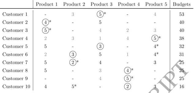
To illustrate the above result, we use the Example 2.2. In Table 2, for every customer k ∈ K, sk
ACCEPTED MANUSCRIPT
Product 1 Product 2 Product 3 Product 4 Product 5 BudgetsCustomer 1 -* 3* 5 * -* 4* 53 Customer 2 4 * -* 5* -* -* 40 Customer 3 5 * -* 4* 2* 3* 40 Customer 4 2* 3* 1* 4* 5 * 38 Customer 5 5* -* 3 * -* 4* 32 Customer 6 2* 3 * 5* 1* 4* 31 Customer 7 5* 2 * 4* -* 3* 25 Customer 8 5* -* 3* 4 * -* 25 Customer 9 -* -* 4* 5 * -* 25 Customer 10 4* 5* -* 2 * 3* 16
Table 2: Preprocessing of the x-variables of Example 2.2
0 by Proposition 6.1, then sk
i appears in gray. If customer k purchases product i in the
optimal solution from Table 1, sk
i is marked with an asterisk. Now, we present how the
preprocessing has been applied for some customers. Since customer 1 is the richest one, by item 1 of the definition ofuwe obtain that u(1) = 3, which is his most preferred product. By applying Proposition 6.1, x1
i = 0 for i ∈ {2,5}. Notice that u(2) = u(3) = 1 by item
2 of the definition of u. In the case of customer 2, his most preferred product has been assigned to customer 1. By applying Proposition 6.1, neither customer 2 nor customer 3 will purchase any product they like less than product 1. If we turn to customer 5, with budget 32 and S5 ={1,3,5}, we remark that for each product iin his list of preferences
there exists another customer k with budget greater than 32 such that u(k) = i (these are, respectively for products 1, 3 and 5, customers 2, 1 and 4). Therefore, u(5) = 3 by item 3 of the definition ofu, and no x-variable related to this customer can be set to zero by Proposition 6.1. Furthermore, comparing with the optimal solution displayed in Table 1, as expected, in this optimal solution every customer k obtains a product he likes more or the same than product u(k).
Remark 6.2. Besides being useful when fixing variables to zero, the proof of Proposi-tion 6.1 derives an optimal soluProposi-tion (˜v,x)˜ from another solution (ˆv,x)ˆ which satisfies
P
i∈Skskix˜ki ≥
P
i∈Skskixˆki ∀k ∈ K, that is, it allows us to obtain an optimal solution in
which customers either buy the same product or buy another one they prefer more. It is also remarkable that there may be more than one optimal solution satisfying Proposition 6.1.
Function u also lets us conclude that some products will not be sold in any optimal solution that satisfies Proposition 6.1:
Corollary 6.3. Let (˜v,x)˜ be an optimal solution of (BNL) or (SLNL) satisfying Propo-sition 6.1. Then for every product i∈I such that u−1(i) =∅, it follows x˜k
i = 0 for every
customer k∈K with i∈Sk, i.e., product i is not sold.