Redistricting Using Constrained Polygonal Clustering

DigitalCommons@University of Nebraska - Lincoln

CSE Journal Articles

Computer Science and Engineering, Department of

2012

Redistricting Using Constrained Polygonal

Clustering

Deepti Joshi

University of Nebraska - Lincoln, [email protected]

Leen-Kiat Soh

University of Nebraska, [email protected]

Ashok Samal

University of Nebraska - Lincoln, [email protected]

Follow this and additional works at:

http://digitalcommons.unl.edu/csearticles

Part of the

Computer Sciences Commons

This Article is brought to you for free and open access by the Computer Science and Engineering, Department of at DigitalCommons@University of Nebraska - Lincoln. It has been accepted for inclusion in CSE Journal Articles by an authorized administrator of DigitalCommons@University of Nebraska - Lincoln.

Joshi, Deepti; Soh, Leen-Kiat; and Samal, Ashok, "Redistricting Using Constrained Polygonal Clustering" (2012).CSE Journal Articles. 101.

Redistricting Using Constrained

Polygonal Clustering

Deepti Joshi, Leen-Kiat Soh,

Member

,

IEEE

, and Ashok Samal,

Member

,

IEEE

Abstract—Redistricting is the process of dividing a geographic area consisting of spatial units—often represented as spatial polygons—into smaller districts that satisfy some properties. It can therefore be formulated as a set partitioning problem where the objective is to cluster the set of spatial polygons into groups such that a value function is maximized [1]. Widely used algorithms developed forpoint-based data sets are not readily applicable because polygons introduce the concepts of spatial contiguity and other topological properties that cannot be captured by representing polygons as points. Furthermore, when clustering polygons, constraints such as spatial contiguity and unit distributedness should be strategically addressed. Toward this, we have developed the Constrained Polygonal Spatial Clustering (CPSC) algorithm based on theAsearch algorithm that integrates cluster-level and instance-level constraints as heuristic functions. Using these heuristics, CPSC identifies the initial seeds, determines the best cluster to grow, and selects the best polygon to be added to the best cluster. We have devised two extensions of CPSC—CPSC* and CPSC*-PS—for problems where constraints can be soft or relaxed. Finally, we compare our algorithm with graph partitioning, simulated annealing, and genetic algorithm-based approaches in two applications—congressional redistricting and school districting.

Index Terms—Spatial clustering, polygonal clustering, constraint-based processing, data mining, spatial databases and GIS

Ç

1

I

R

space or region of spatial units often represented as polygons into smaller subregions or districts. As such, it can be viewed as a set partitioning problem, i.e., the problem is to cluster the entire set of spatial polygons into groups such that a value function is maximized [1]. Because of the spatial properties involved, redistricting is akin to spatial clustering. Meanwhile, as the most common use of these districts is to facilitate some form of jurisdiction, redistrict-ing often involves satisfyredistrict-ing or conformredistrict-ing to constraints that represent policies, laws and regulations. Typical spatially flavored constraints are spatial contiguity and compactness, while an example of domain-specific con-straint is uniform population (or resource) distribution.

Spatial clustering deals with spatial data that is generally organized in the form of a set of points or polygons. Most spatial clustering algorithms proposed in the literature focus on clustering point data [10]. However, when applying these algorithms to cluster polygons instead of points, these algorithms fall short of giving accurate results [12], [13]. The main cause of the inadequacy is that in comparison to polygons, points are relatively simpler geographic objects. Polygons, especially in the geographic space, share spatial and topological relationships and cannot be accurately represented as points. For example, two polygons may share boundaries with each other, or may cover different amounts of area. None of these conditions can be captured in point

data sets. Redistricting is thus a polygonal spatial clustering problem as most of the space around us is divided into polygons, e.g., states, counties, census tracts, blocks, etc. While, a few algorithms have been proposed in the past for polygonal spatial clustering [12], [13], [15], [21], all these algorithms perform clustering as a form of unsupervised learning, whereas redistricting requires the use of some form of domain knowledge. Efficient use of this available informa-tion can significantly enhance the quality of the clusters. Use of constraints in clustering is widely examined in data mining. Examples of constraint-based clustering algorithms are COP-KMEANS [23], C-DBSCAN [19], etc. However, once again these algorithms are allpointbased, and therefore do not provide the framework to take into consideration the spatial and topological properties of polygons.

In this paper, we present a suite of clustering algorithms for clustering polygons in the presence of constraints. The core algorithm, called the Constrained Polygonal Spatial Clustering (CPSC) algorithm, is designed to solve the problem when the constraints are hard and inviolable. We further propose two extensions of CPSC, namely, CPSC* and CPSC*-PS (i.e., CPSC* with Polygon Split). CPSC* is designed to handle soft constraints, while CPSC*-PS is a further extension to allow a polygon to be split during the clustering process using an underlying tessellation in order to improve the quality of the clustering results. The uniqueness of these algorithms is that they make use of the spatial and topological relationships between the polygons as well as the domain knowledge present in the form of constraints to cluster polygons using anA search-like underlying process. We also consider two types of constraints. Instance-level constraints, such as must-link and cannot-link constraints [6], are applied to individual objects being clustered. Cluster-level constraints, on the other hand, are applied to the cluster as a whole. Some cluster-level constraints are averaging or summation con-straints [7]. Briefly, the core algorithm CPSC is divided into

. The authors are with the Department of Computer Science and Engineering, University of Nebraska-Lincoln, Avery Hall, Lincoln, NE 68588-0115. E-mail: {djoshi, lksoh, samal}@cse.unl.edu.

Manuscript received 29 June 2010; revised 15 Mar. 2011; accepted 9 June 2011; published online 23 June 2011.

Recommended for acceptance by J. Sander.

For information on obtaining reprints of this article, please send e-mail to: [email protected], and reference IEEECS Log Number TKDE-2010-06-0357. Digital Object Identifier no. 10.1109/TKDE.2011.140.

three main steps: 1) select seeds, 2) decide the best cluster (BC) to grow, and 3) select the best polygon (BP) to be added to the best cluster. Several novel strategies of the algorithm include

1. Use of heuristic functions to apply the constraints during clustering where a heuristic function incorporating the distance of the current state of the cluster from the desired goal, and the cost in the form of reduction in the flexibility of the growth of all the other clusters to facilitate efficient use of constraints;

2. Integration of constraints in seed selection andselection of the best cluster to growbased on a cluster’s need to grow to make the algorithm more robust to order dependency and poor initial seeding;

3. Selection of the best polygon to be added to the best cluster is done in a manner that will have minimal impact on the growth of surrounding clusters; and

4. Built-in back-tracking system within the algorithm by allowing the polygons to move from one cluster to another to avoid getting stuck at local optima. Further, based on CPSC, CPSC* finds a solution by considering prioritization and relaxation of con-straints to allow un-clustered polygons to be assigned to clusters. CPSC* also has a deadlock detection and breaking mechanism to ensure con-vergence. Finally, CPSC*-PS allows for splitting individual polygons to improve cluster quality. For our comparative and validation study, we apply the CPSC suite to two widely used redistricting problems:

congressional redistrictingandformation of school districts. We compare the results of CPSC for the congressional redis-tricting problem with three other techniques based on graph partitioning [4], simulated annealing [17], and genetic-based algorithms [2]. In our study, we find that our algorithm outperforms the other three algorithms by producing districts that have almost equal population and are spatially compact.

Note that this work is an extension of [14]. While in [14] we present a version of the algorithm CPSC and its application to the congressional redistricting problem, here we refine and extend our comparison of CPSC to the genetic algorithms (GAs) for redistricting. Also, we present two additional versions of CPSC and apply our algorithm to the school district formation problem to more comprehensively evaluate our algorithms.

2

R

W

Redistricting is essentially an optimization problem where the global optimum solution is difficult to find. This is because the size of the solution space can be enormous. A simple brute force search through all the possible solutions is impractical especially when the data set size increases. Moreover, due to the size of the real data sets, most of the current techniques used for automated redistricting resort to unproven guesswork [1] and random selection, and are therefore inefficient and may not be accurate. To solve redistricting problems, several metaheuristic approaches have been proposed: graph partitioning, simulated anneal-ing, and genetic algorithm-based redistricting methods.

While these algorithms work with polygonal data sets, they do not exploit the spatial properties of the polygons, or the nature of the geographic space. These methods are discussed here and further evaluated in Section 5.

2.1 Redistricting Approaches

The problem of partitioning a geographic area into a collection of contiguous, approximately equal population districts has been viewed as a graph partitioning problem. The graph is formed by representing each polygon as a node, and the polygons that share boundaries are connected by an edge. Further, each node is assigned a weight equal to the population of the polygon. The problem is to partition the graph into a fixed number of subgraphs or clusters such that the sum of the node weights within each cluster is equal, and each cluster is connected. A graph partitioning algorithm for congressional redistrictinghas been presented in [4]. The advantages of this approach are that it is computationally fast, and it presents the user with several potentially useful plans. However, there are several disadvantages with this approach:

1. The random selection of seeds may lead to the development of poor plans.

2. There are no guidelines provided in this methodol-ogy to select the best plan.

3. This method does not work well when the number of seeds is large as the total number of plans that may be produced scales up very fast.

4. There is no intuitive way to incorporate intracluster constraints during the clustering process.

Other approaches include the use of simulated anneal-ing. Simulated annealing is a general purpose optimization procedure based on the thermodynamic process of anneal-ing of metals by slow coolanneal-ing. An example algorithm for the redistricting problem is theSimulated Annealing Redistricting Algorithm (SARA) [17]. While simulated annealing-based methods perform better than informal or manual methods, they have several disadvantages:

1. An initial solution needs to be provided to the algorithm.

2. The final solution produced is therefore heavily dependent on the initial plan provided to the algorithm.

3. More than one spatial constraint cannot be easily incorporated in algorithms such as SARA.

4. There are no guarantees that a global optimum will be found.

Further, genetic algorithms have also been used inzone designing. GAs are a subset of the evolutionary algorithms based on Darwin’s theory of evolution. The basic idea is that each solution to the problem is coded as a bit string, taken to be a chromosome, possibly with a number of substrings that act as genes. At any given point in time, a number of such chromosomes are kept where each chromosome represents a solution to the problem. Natural selection is simulated by evaluating the fitness of each solution, measured by how well it solves the problem at hand, and giving the best individuals a higher probability of remaining in the solution pool during the next generation. An application of GAs to

zone designing is given is [2]. The algorithm takes as input a point representation of each polygon, and the number of zones or clusters (k). A polygon is represented using its centroid. The disadvantages of GAs are as follows:

1. They need many more function evaluations than linearized methods.

2. A lot of care needs to be taken while designing the encodings.

3. There is no guaranteed convergence even to a local minimum.

4. Finally, GAs cannot be applied to problems where the seeds are fixed and thus only one chromosome in the initial population pool.

2.2 Comparison with the CPSC Family

The CPSC family of algorithms addresses several of the disadvantages of the approaches discussed in Sections 2.1, 2.2, and 2.3. The CPSC family does not require an initial input plan, i.e., an initial solution where every polygon is assigned to a district or cluster, to work upon, as is the case with SARA and the genetic algorithm for zone design. For example, for the congressional redistricting problem, SARA takes as input a set of districts with every polygon in the data set assigned to a district, which are spatially contiguous but do not satisfy all the constraints such as the equal population constraint. SARA then improves upon this initial plan so that all the districts satisfy the constraint of equal population. The GA for zone design also follows a similar approach where it begins with taking a set of input plans. Here again, each input plan is a possible solution to the congressional redistricting problem where each polygon in the data set is assigned to a district. It then evaluates the fitness of each plan, based on the chosen fitness function and contiguity check, and applies selection, crossover, and mutation operators until it finds a solution that meets the stopping criterion. The CPSC family, on the other hand, selects seeds from the data set and then grows the clusters with the seeds as the starting points of the clusters. The seeds are simply single polygons selected as for growing clusters, and therefore do not constitute an input plan.

The CPSC family also defines a clear methodology to select seeds based on a predefined set of constraints, as opposed to the random selection of seeds by the graph partitioning algorithm. Most importantly, the CPSC family can incorporate any type of spatial or domain-specific constraints in the clustering process by the use of its heuristic function and other guidelines as defined in Section 3, and demonstrated in Section 4. There is no intuitive way to incorporate spatial constraints such as minimum distance between the seed and other polygons within the cluster within SARA and GA. SARA randomly makes its move in order to avoid local optima; however, it has the risk of getting stuck at the local minima. As the CPSC family follows theAsearch-like mechanism in order to grow the clusters, there is no risk of getting stuck at the local minima. Finally, CPSC can also easily be modified to work with fixed seeds, i.e., the seeds of the cluster cannot be changed or moved during the clustering process. A GA will not work in this situation as the input population cannot be formed in this case.

3

C

P

S

C

A

The main aim of our Constrained Polygonal Spatial Clustering algorithm is to grow clusters, satisfying con-straints that can be used for spatial analysis and map formation. In order to facilitate the purposes of jurisdiction within a cluster that represents a district, the algorithm is designed to inherently produce spatially contiguous and compact clusters. This knowledge is embedded in the clustering process in the form of constraints. The clusters are grown using an iterative,A-like search process.

3.1 Preliminaries

A search algorithm. A is the best first search algorithm that finds the least costly path from an initial node to the goal node [20]. It uses a heuristic function (FðnÞ ¼GðnÞ þ

HðnÞ) that is a combination of a path cost function (GðnÞ) and an admissible distance function (HðnÞ) i.e., a distance function that does not overestimate the distance to the goal. The path cost functionGðnÞmeasures the cost of arriving at the current node from the initial node, and the distance function HðnÞ measures the estimated distance from the current node to the goal node. Starting with the initial node, A maintains a priority queue of nodes to be traversed, known as the open set, or OPEN. The lower

FðnÞfor a given nodenis, the higher is its priority. At each step of the algorithm, the node with the lowestFðnÞvalue is removed from the OPEN queue and added to another queue known as the closed set, or CLOSED. TheF andH

values of its neighbors are updated accordingly, and these neighbors, which have not been already added to OPEN or CLOSED, are added to the OPEN queue. The algorithm continues until a goal node is discovered (or until the OPEN queue is empty).

Spatial contiguity. A cluster of polygons is spatially contiguous when every polygon within the cluster shares at least a part of its boundary with at least one other polygon within the cluster. In other words, the number of connected components for a spatially contiguous cluster will always be 1.

Cluster compactness. Compactness is most commonly measured as an attribute of the shape of the cluster. A circle is the most compact shape for any cluster because it covers the most area within the smallest perimeter [5]. We define a compact cluster as a cluster that has a shape very close to that of a simple geometric shape and does not meander in space forming a snake or river like structure. Examples of simple geometric shapes are circle, rectangle, and square. Different measures have been defined in order to compute the cluster compactness. For example—radial compactness measures the compactness of a cluster as the sum of euclidean distances between the centroid of its polygons and the centroid of the cluster itself (dij).

Constraints. In many cases, there is some domain knowledge present. Instead of simply using this knowledge for validation purposes, it can also be used to “guide” or “adjust” the otherwise unsupervised clustering process [9]. The resulting approach is known as the semi-supervised clustering [8] or the process of constraint-based clustering. Constraints applied during the process of clustering can be of two types—instance-level constraints and cluster-level

constraints. Instance-level constraints are applied to the individual objects being clustered. There are two types of instance-level constraints, namely, must-link constraints and cannot-link constraints [24]. Briefly, the must-link constraints are the set of constraints that are satisfied by the polygons that must belong to the same cluster. On the other hand, cannot-link constraints are satisfied by a pair of polygons only if both the polygons are members of different clusters.Cluster-level constraintsare applied to the cluster on the whole. Examples of cluster-level constraints are averaging or summation constraints [6]. For example, in the formation of school districts, within a district each polygon must be at most x distance away from the school polygon. This will be categorized as a cluster-level constraint because it pertains to grouping “related” polygons into the same cluster. Other examples include the constraints of spatial contiguity and compactness.

Heuristic function based on constraints. In order to incorporate the different types of constraints within the clustering process, the idea of a heuristic function (F), borrowed from heuristic search algorithms, is used. F is a combination of: 1) A function H that approximates the distance of the current state of the cluster to the goal state thereby measuring the level of need of the cluster to grow further, and 2) A cost function G that measures the reduction in flexibility on the growth of the clusters. Using the above,F is defined as a sum of the two, that is,

F ¼HþG: ð1Þ

The distance function H takes into account the cluster-level constraints to find the distance of the current state of the cluster from its target state, and the cost function G

looks at the effect of the growth of every cluster on the other clusters. Using this combination ofHandG, CPSC is able to decide which cluster to grow, or which polygon to add to the selected cluster. The reduction in the flexibility of the growth of the clusters is viewed as a cost function because a choice based onHalone may have an adverse effect on the growth of the remaining clusters. With the addition ofGto

H, we penalize a node if it restricts the growth of other clusters. In other words, we prevent CPSC from following a

purelygreedy approach.

In order to select the distance function (H) that approximates the distance of the current state of the cluster to the goal state, the first step is to identify which constraints are easily quantifiable, and those which describe the desired properties of the target clusters. For example, while forming congressional districts, we can formulate our target clusters to be spatially contiguous and compact clusters with equal population. Next, the cluster-level constraints are identified. For example, among the most important constraints identified for the congressional redistricting problem, the constraints of equal population and spatial compactness are cluster-level constraints, while the spatial contiguity can be most easily translated into instance-level constraints. Using the selected cluster-level constraints, the distance functionHcan be defined as

H¼d1ðCurrent Cj; T arget CjÞ þd2ðCurrent Cj; T arget CjÞ þ þdxðCurrent Cj; T arget CjÞ;

ð2Þ

where dxðCurrent Cj; T arget CjÞ is the distance between

the current state of clusterCjand the target state of cluster

Cj based on cluster-level constraint x. Thus, for the

congressional redistricting problem, the distance function H is defined as

H¼Req P opCurrent P op

Req P op

þT arget CompactnessCurrent Compactness

T arget Compactness ;

ð3Þ

where Req Pop is the expected total population of each cluster. The constraint of cluster compactness dictates that the cluster must grow to form the most compact district. As stated before, a district with a circular shape would be the most compact. The compactness index of a circle measured using the Schwartzberg’s index [22] (defined as the ratio of the square of the perimeter and the area) will always be4. Thus, T arget Compactness¼4. The Current Pop, and the

Current Compactnessare the measures of the current state of the cluster.

With the use of the cost functionG, our objective is to select a cluster to be grown that will preserve the maximum degree of flexibility for the other clusters to grow. This function is mostly dictated by the domain-independent constraints of assigning every polygon to a cluster, and forming spatially contiguous and compact district. As example of a cost functionGis as follows:

G¼ max

i¼0to k jmax¼0to n½ðOðCiÞ O

0_ðC

i;jÞÞ=ðOðCiÞÞ; ð4Þ

where k is the number of clusters, n is the number of polygons surrounding a cluster—i.e., neighbors—that have not yet been assigned to any cluster, OðCiÞ is the (outer)

boundary of a cluster i(assuming all polygons within the cluster are contiguous) that is shared with polygons that are still not assigned to any cluster, and,O0ðCi;jÞis the resulting

new boundary of the clusteriafter adding a new polygonj. Intuitively, this cost function says that if adding a new polygon makes it more compact—such as filling up a concave segment of the old boundary—then the cost will be negative (lowered); otherwise, the cost will be positive as the cluster is growing more aggressively reducing the flexibility of the growth of other clusters. This cost function will promote parallel cluster growth.

In Sections 4 and 5 where we apply our algorithm to the congressional redistricting problem and the school district formation problem, spatial contiguity and cluster compact-ness are important properties of the desired target clusters. As a result, we chose the cost function based of the extent of the open boundary of the clusters defined in (4), as this cost function penalizes the clusters the most if they are not spatially compact, and are instead distributed in space.

In summary, it should be noted that ifH overestimates the distance of the current state of the cluster from the target state, the clustering process will not jump from one cluster to another. It will instead grow one cluster at a time. Therefore, the clustering process will become sequential. On the hand, if H underestimates the distance then the clustering process will become considerably slower. Simi-larly, a more stringent cost function will result in a slower clustering process with every cluster selecting a polygon to grow very conservatively and vice-versa.

3.2 The CPSC Algorithm

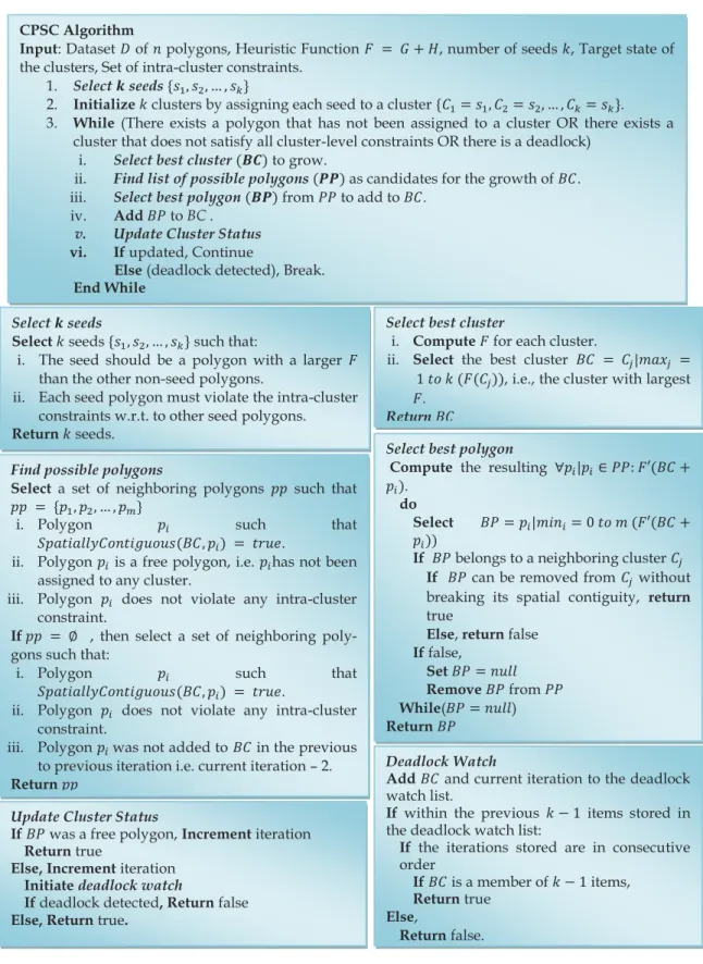
The CPSC algorithm (Fig. 1) is a generic algorithm that is designed to be applicable to any domain given the data set of polygons, the number of clusters, a set of constraints, and the heuristic function F based on the constraints. CPSC begins by selecting seeds from the data set. As each seed will be grown to form a cluster, every seed represents a separate cluster. Because of that, the seed selection follows a

counterintuitive path where every seed polygon must violate all must-link constraints w.r.t. to other seed polygons. Other-wise, the resulting seeds may be clustered within the same cluster, making the initial seeding invalid. Thus, the seeds are selected from the data set using a systematic search based upon the available domain knowledge, which are represented as heuristics, for example, the pairwise distance between the polygons, the population of each polygon, the

area covered by each polygon, etc. Based on the desired properties of the target clusters, the most important constraint as identified by the domain experts is selected, and the corresponding property used in the constraint is implemented and computed for each polygon. Next, the polygons are sorted in ascending order based on the computed property. Then, we select the top kpolygons in the sorted list that 1) violate the must-link constraints such as spatial contiguity, and 2) abide by any cannot-link constraints, wherekis the predefined number of clusters to be detected.

Once the seeds are selected, the initial clusters come into existence, and a search process can begin. Adopting theA -search algorithm, we assume that the initial clusters (consisting of the individual seeds) are the start state, and the target clusters are the goal state. Each cluster is then grown from the start state by adding polygons to the cluster one by one until the target cluster state is achieved. Adapting this search paradigm, at the beginning of every iteration the best cluster to be grown is selected. To achieve this, a heuristic function (F) is used (cf. Section 3.1). CPSC selects the cluster with the biggest need, that is the cluster with the largestF.

Upon the selection of the best cluster, the next step is to select the best polygon to be added to the best cluster. Toward this, first a set of potential polygons (PP)is selected that may be added toBC. This set consists of all previously unassigned, spatially contiguous neighboring polygons to

BC, i.e., the polygons that share their boundary with BC

(SpatillyContiguousðBC; piÞ ¼true), and have not been

assigned to any cluster so far. In case there are zero unassigned polygons remaining within the neighborhood ofBC,then the neighboring polygons from the neighboring clusters, i.e., the clusters sharing some portion of their boundary with BC, are selected as potential polygons for

BC. Every polygon within this set must abide by each intracluster constraint. A selection between them is then made on the basis of the heuristic function F0. F0 is once again a combination of 1) a function (H0_{) that approximates}

the distance of the current state ofBCto the goal state after the addition ofBP, and 2) a cost functionðG0Þthat measures the reduction in flexibility on the growth of BC after the addition of BP. Here, CPSC selects the polygon that contributes most to the cluster, in other words, satisfies its need the most. Therefore,BP is the polygon that results in the smallestF forBC. This alternating strategy of selecting the cluster with the largestF asBC, and then selecting the polygonBPas the polygon that results in the smallestF for

BC, allows every cluster to grow simultaneously, therefore giving every cluster the equal opportunity to select the best polygon for itself. If, on the other hand, BC would be selected as the cluster with the smallestF, then the clusters would be forced to grow sequentially, and the property of compactness will be lost.

After BP is selected to be added to BC, if BC and its neighboring clusters are spatially contiguous, the selected polygon (BP) is added to the best cluster. This process goes on until: 1) all the polygons within the data set have been assigned to a cluster, and the target state clusters are produced that satisfy the given set of constraints, OR 2) the algorithm enters the state of a deadlock. A deadlock occurs

when a cluster adds a polygon, then loses the polygon to another cluster, and then regains the same polygon over and over across successive iterations in a “tug-of-war” with another cluster. Formally, we define a set of clusters (C1rk) to be in a deadlock when at iteration I a cluster

Cr is at state x, and at iteration J, where JIk, the

cluster Cr is at state x again. The state of a cluster at any

iterationIrefers to the polygons that are the members of the cluster at iterationI.

3.3 Extensions of CPSC

CPSC does not guarantee convergence, i.e., every polygon may not be assigned to a cluster, because of the search process is cluster centric instead of instance or polygon centric. First, we define convergence as follows: an algorithm is said to converge when every polygon pi2D,

whereDis the complete data set, is assigned to a clusterCj,

i.e.,8p1in9C1jkjpi2Cj. Ifthe problem allows constraints to

be softened or relaxed, then, in order to guarantee conver-gence, we propose another algorithm known as CPSC*. Furthermore, we proposeCPSC*-PSto split a polygon into two to better satisfy constraints.

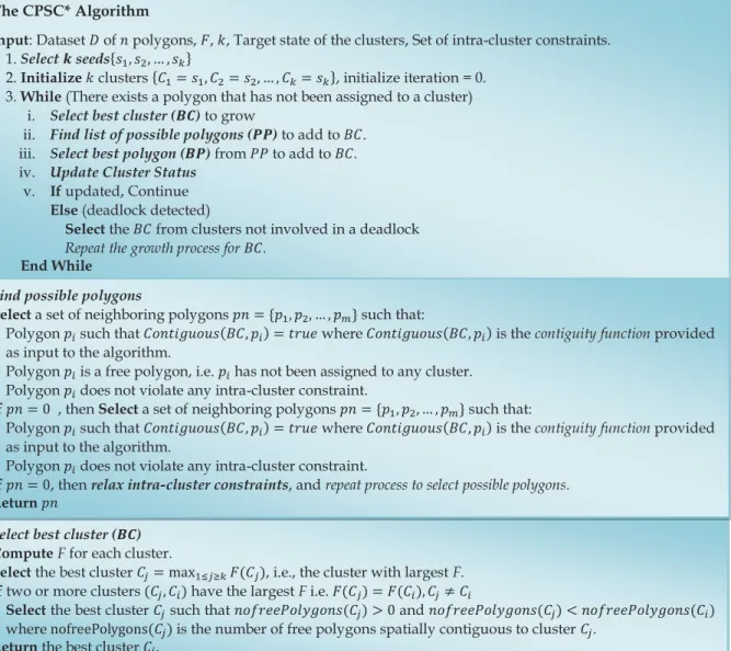
3.3.1 CPSC*

The CPSC* algorithm (Fig. 2), follows a similar approach to grow clusters. However,CPSC* allows the users to relax their constraints to ensure that every polygon gets assigned to a cluster. First, CPSC* uses a weighted distance function

H—thereby converting the hard cluster-level constraints to soft cluster-level constraints, and allowing the user to prioritize the constraints. And second, while selecting the potential polygon set to grow a cluster, CPSC* checks that all must-link constraints are met. However, if the best cluster has not achieved its target state, and there are no more polygons left that satisfy the required constraints, then these constraints are relaxed, so that the remaining unassigned polygons may become potential members of

BC. For example, if there is a constraint that states that every polygon within the cluster must be at most 10 miles away from the seed polygon, and there are polygons within the data set that are more than 10 miles away from every seed, these polygons will never get assigned to a cluster. To overcome this situation, the user may relax the constraint and define the threshold distance to be increased by 2 miles at a time. The weighted distance functionHis

H¼w1d1ðCurrent Cj; T arget CjÞ

þw2d2ðCurrent Cj; T arget CjÞ þ þwx dxðCurrent Cj; T arget CjÞ;

ð5Þ

wheredxðCurrent Cj; T arget CjÞis the distance between the

current state of clusterCj and the target state of clusterCj

based on cluster-level constraint x, and wx is the weight

assigned to cluster-level constraintx.w1þw2þ þwx¼1.

The weights are assigned according to the priority of the constraints, and are user defined. The weighted distance function used by CPSC*, therefore, allows the user the flexibility to guide the growth of the clusters based on selected constraints, as opposed to the distance function used by CPSC that enforces every constraint equally on the clustering process.

Furthermore, in the worst case scenario, CPSC may lead to a situation where two or more clusters enter a deadlock. If this happens, the algorithm will not converge. In order to avoid deadlocks, CPSC* initiates adeadlock watchas soon as a cluster adds a polygon that was previously assigned to another cluster. The deadlock watch stores the current state of the cluster. If acrossk1consecutive iterations, the two or more clusters repeat the same state, a deadlock is detected. CPSC* then breaks the deadlock by forcing another cluster not involved in the deadlock to grow.

Theorem 1.CPSC* guarantees convergence.

Proof. Let us assume that there exists a polygon

pijpi 62 Cj; 1jk, but CPSC* either 1) has stopped

executing, or 2) has resided in a deadlock permanently. In case 1, assuming that CPSC* has stopped executing would imply that every polygons has been assigned to a cluster. This is because CPSC* continues to grow all clusters until there exists a polygon that has not been assigned to a cluster. As polygon pi has not yet been

assigned to a cluster, CPSC* will not stop executing. The only condition when pi will not be assigned to it’s

neighboring cluster, let’s say Cj, if some other cluster

Cy’s F is greater than Cj’s F. Due to the properties of

deadlock detection and breaking, and soft intracluster constraints, CPSC* guarantees that a polygon will be added to a cluster until there exists a free polygon. Thus, the condition FðCjÞ> FðCyÞ will become true

even-tually. When this happens polygonpiwill be assigned to

cluster Cj, and since every polygon has now been

assigned to a cluster, CPSC* will stop executing. Thus, when CPSC* stops executing, every polygon will be assigned to a cluster.

In Case 2, assuming that CPSC* has resided in a deadlock permanently would imply that there does not exist a cluster that is not involved in the deadlock. This further means that none of the clusters have any free polygons that are contiguous to them. In this case, all polygons would already be assigned to a cluster, and the algorithm would have converged. Thus, CPSC* cannot reside in a deadlock permanently. Hence, our assump-tion has to be false for either case. Therefore, using proof by contradiction, we conclude that CPSC* guarantees

convergence. tu

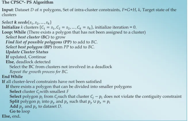
3.3.2 CPSC*-PS

In order to guarantee convergence, CPSC* forces the hard constraints to be converted to soft constraints. To improve the quality of the results obtained by CPSC* such that the solution may come closer to satisfying the hard constraints, we propose an extension of CPSC* known as CPSC*-PS, where PS stands for Polygon Split. The assumption that CPSC*-PS makes is that the polygons can be divided into smaller polygons. Fig. 3 presents an outline of the algorithm. Once all the polygons have been assigned to a cluster, if the hard cluster-level constraints have not been satisfied, then CPSC*-PS selects a polygon from the cluster with the smallestF to be removed. This polygon is divided into two smaller polygons based on the underlying tessellation, and added to the data set as unassigned polygons. CPSC*-PS then repeats the process of assigning these polygons to the clusters. This process is repeated until all cluster-level constraints have been satisfied, or until there exists a polygon that may be divided into smaller polygons. Note also that the functions (for example, Selectkseeds, etc.) for CPSC*-PS are the same as CPSC*, and therefore are not defined here again. Furthermore, as initially the algorithm uses CPSC* to produce clusters that are further improved upon using the polygon-split mechanism, and CPSC* guarantees conver-gence, CPSC*-PS also guarantees convergence.

3.4 Comparison of CPSC, CPSC*, and CPSC*-PS

While CPSC is the core algorithm for both CPSC* and CPSC-PS_{, all three algorithms handle different types of}

problems as follows:

1. CPSC is designed for problems where a solution exists within the data set and all constraints arehard.

For example, CPSC has been applied to the congres-sional redistricting application in Section 5.1, which is a problem with hard constraints, as described in Section 4.1.

2. CPSC*, on the other hand, allows the user to

prioritizeconstraints, and works withsoftconstraints. Thus, it is especially appropriate for problems that allow for constraints to be relaxed to obtain a suboptimal solution when an optimal solution is not possible. For example, CPSC* has been applied to the school district formation problem in Section 5.2, which is a problem with soft constraints, as described in Section 4.2.

3. CPSC*-PS is an extension of CPSC* where the goal is to further improve the suboptimal solution found by CPSC* by splitting a polygon into two or more

smaller polygons—essentially allowing parts of the same polygon to be assigned into two or more clusters to satisfy constraints more closely. Thus, CPSC*-PS can be applied only in situations where an underlying tessellation of polygons exist. For exam-ple, CPSC*-PS has been applied to a synthetic data set in Section 5.2.

3.5 Computational Complexity of CPSC

In the best case scenario, CPSC assigns each polygon within the data set to the best cluster in the first assignment. In this case, the computational complexity of the algorithm can be computed in two steps; the seed selection process is carried out in Oðn log nþkÞ number of steps in the best case scenario, andOðn log nþnkÞ number of steps in the worst case scenario, wherenis the number of polygons within the data set, andkis the number of clusters to be formed. The

cluster growth process can be accomplished inOðnðkþmÞÞ

wherem is the maximum number of neighbors of the best cluster. However, in the worst case scenario, CPSC will either enter a deadlock and exit without assigning all the polygons within the data set to the appropriate clusters, or every polygon will need to be reassigned to another cluster after it has already been assigned to the best cluster. In the second case, the worst case computational complexity of CPSC isOðn2Þ ask m, andm n.

4

A

R

-W

P

In order to show the usefulness of our algorithm, we have applied CPSC and its extensions to two real-world problems: 1) congressional redistricting and 2) formation of school districts. Both these problems can be interpreted as problems of cluster formation where each cluster represents a district. Each district or cluster is formed by grouping together polygons that follow certain constraints. Details of both the problems along with the constraints applied in both cases are described next.

Note that in our representation of the congressional redistricting problem, as all constraints are hard, we use the CPSC algorithm. For the school districts problem, as there is a mixture of hard and soft constraints, we use the CPSC* variant.

4.1 The Congressional Redistricting Problem

Congressional redistricting has been a vexing problem for a long time. Once a state learns that it has been assigned

k seats, it must divide its territory into k districts. This division is a geometric one where there can be several ways of dividing the state territory into k districts [11]. This opportunity of being able to divide using several different methods leads to the phenomenon of political gerryman-dering where any party could form districts for their own advantage.

The constraints that define a “good district” are as follows:

1. All the districts within a state should be equal in population,

2. Each district should be a single continuous territory,

3. Districts should be compact; Tentacles wriggling through the landscape are considered a bad design,

4. Districts should recognize the exiting communities of interest,

5. Districts should conform to existing natural and political boundaries when possible, and

6. Finally, under the US Voting Rights Act, a district must not be drawn with the intent of excluding the minority candidates from election.

In case of any conflict among the above constraints, the highest priority is given to numerical equality and spatial contiguity. In our implementation, we take into considera-tion only the first three constraints as they define the overall structure of the algorithm. Constraints 4, 5, and 6 are not incorporated due to lack of data. However, they can be applied as must-link and cannot-link constraints while selecting the possible set of polygons in step 3(c) of the algorithm.

Therefore,the problem statement is to divide the geographic area of a state intokdistricts such that the total population within each district is nearly equal or within 1 percent margin of error (M.O.E). Each of thesekdistricts must be spatially contiguous. Finally, all of thekdistricts must be as compact as possible.

4.1.1 Heuristics Used

The heuristic function F used by CPSC in order to determine the best cluster to grow, and the best polygon to add to the best cluster is defined based on the input data set, and the constraints defined before the clustering process. For the congressional redistricting problem, the inputs to the algorithm are: Census Tracts of US as the set of polygons, k—defining the number of seeds, and the following set of constraints: Cluster-level Constraints: CS1. Each cluster must be spatially contiguous, CS2. Each cluster must be compact, CS3. Each cluster must contain equal population of x, with a margin of error of 1 percent.

Instance-Level Constraints:CS4. Set of spatial constraints as a set of must-link constraints between the census tracts, CS5. Set of spatial constraints as a set of cannot-link constraints between the census tracts.

All the constraints mentioned above are hard constraints. Based on the above inputs, we define the heuristic function

F ¼GþH, whereH, defined in (3) in Section 3.1, measures the need for the respective cluster to grow further, andG, defined in (4) in Section 3.1, is the cost of the reduction in the flexibility of the growth of the cluster. Thus, together withH, the best cluster (i.e., the best cluster that should be selected to grow) is one with the highest value of F, meaning one that is 1) furthest away from the target population and/or the least compact, and 2) the costliest to grow (akin to the min-conflict algorithm in conventional constraint satisfaction problems).

As alluded to earlier, we use the same rationale in designing the cost functionG0for measuring the reduction in the flexibility of the growth of the best cluster while selecting the best polygon to add to the best clusterCi as

G0¼X

k

i¼0

½ðOðCiÞ O0ðCi;jÞÞ=ðOðCiÞÞ: ð6Þ

To select the best polygon to add to a cluster, we select the neighbor that reduces the open boundary of the cluster the most, and takes the cluster closest to its target. Thus, together with H0, the best polygon will 1) increase the population of the cluster, 2) make it more compact, and 3) reduce the open boundary of the cluster.

Note that while we use a maximum function in (4), we use a summation function in (6). This is because when a free polygon (i.e., a polygon not yet assigned to any cluster) is added to a cluster, this action may considerably hinder the growth of another cluster. Therefore, we include the cumulative effect of the addition of a polygon to a cluster. Taken together, (4) allows us to pick the least costly cluster to grow, and (6) allows us to pick the least costly neighbor to add to that cluster.

Seed selection.Also, when computingF for identifying the seeds in the first place, since each “cluster” consists of only one polygon, the compactness measure is the same for each cluster (i.e., ¼1) and G is also the same for each

cluster. Thus, selecting the seeds from the data set reduces to the problem of sorting the polygons by F ¼H¼

xcurrent popin descending order and selecting the top

k polygons. Furthermore, as the seeds cannot be spatially contiguous, a physical distance between them is enforced as follows: the physical distance between two seeds must be a function of rand kunless specified otherwise. That is, for seedssi andsj, the distance between them

distðsi; sjÞ ¼fðr; kÞ; wherer¼ ffiffiffiffiffiffiffiffiffiffiffiffiffiffiffiffiffiffiffiffiffiffiffiffiffiffiffiffiffiffiffi Area of MBR k r : ð7Þ

Area of MBRis the area of the enclosing minimum bounding rectangle of the data set, andkis the number of seeds.

4.2 The School District Formation Problem

A school district is a geographic area in which the schools share a common administrative structure. School districts are formed to ensure that no school is burdened with too many students, and that no student has to travel far to go to school. Therefore, each school district will approximately have a certain number of students, and every household will be within a certain distance from a school.

The formation of school districts is important because school districts hold great importance in the legislature of the community. The functioning of a school district can be a key influence and concern in local politics. A well run district with safe and clean schools, graduating enough students to good universities, can enhance the value of housing in its area, and thus increase the amount of tax revenue available to carry out its operations. Conversely, a poorly run district may cause growth in the area to be far less than surrounding areas, or even a decline in population [18]. Over the years due to new developments, populations have shifted and occupied new land. As a result, there are cases where an existing school district is overburdened with students.

The problem statement is, therefore, to divide the geographic area of a state into districts such that each district has almost equal number of students, and every household must be within a threshold distance from the public school in the district.

4.2.1 Heuristics Used

In the school district formation problem, similar constraints that we see in the congressional districting problem apply: Census Blocks as the set of polygons, and a set of constraints. However, only spatial contiguity is a hard constraint. The equal population and compactness are soft constraints, because it is more necessary to assign every polygon to a cluster or school district in this case, rather than equal population and compactness. Other than these constraints, there is an added intra-cluster constraint of the threshold distance from the school polygon, i.e., every polygon within the school district must be no more than the threshold distance away from the polygon within which lies a school. This constraint is also a soft constraint, such that the threshold distance increased to guarantee convergence. Finally, the last constraint that applies to this problem is that the seeds will be fixed as the school polygons. This constraint is a hard constraint because the schools cannot be moved. Based on the above inputs, we define the heuristic function F as follows: F¼GþH,

where¼w1

ðReq P opCurrent P opÞ

Req P op þw2

T arget CompactnessCurrent Compactness

T arget Compactness ;

ð8Þ

w1þw2¼1; Required population is the total population

divided by k; G is the same function as defined for the previous problem. Similarly, F0 _{for selecting the best}

polygon is also the same. As the seeds are fixed for this problem, we do not need to execute the step to select seeds usingF. The threshold distance between the polygons and the seed polygons is an intracluster constraint, and is therefore enforced when selecting potential polygons to be added to the best cluster as defined in Section 3 for the CPSC* algorithm.

5

E

E

In this section, we evaluate the CPSC algorithm suite by applying it to two well-known redistricting problems— congressional redistricting as defined in Section 4.1 and the school district formation problem as defined in Section 4.2. We also compare our results for the congressional redis-tricting problem with the results obtained by the graph partitioning, the simulated annealing algorithm (SARA), and the GA for zone design described in Section 2. Also, we examine the behavior of CPSC and CPSC* in these two experiments, and apply CPSC*-PS to improve the quality of the clusters obtained by the CPSC* algorithm.

5.1 Evaluation of CPSC on the Congressional Redistricting Application

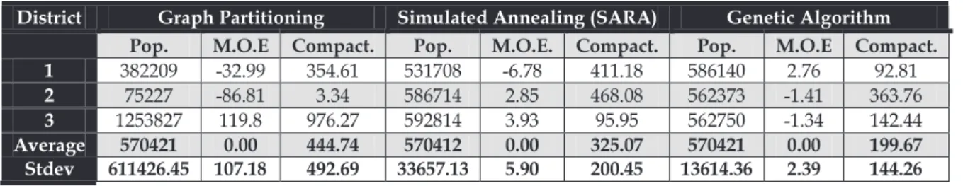
State of Nebraska.For this experiment, we used the census tract data set for the state of Nebraska. The total number of polygons (census tracts) in Nebraska is 505. The state of Nebraska has been assigned three seats in the congress. Thus,k¼3. The approximate population of each cluster or district must be equal to 570,421 within a 1 percent margin of error. Fig. 4a shows the initial clusters formed based on a random run, and the final clusters produced in step 2 of the graph partitioning algorithm (Section 2.1). Figs. 4b and 4c present two random input plans and the respective results obtained upon the application of SARA (Section 2.2). The input plans were selected with the following constraints:

1. Every input district or cluster is spatially contiguous.

2. The structure of every input district is fairly compact to begin with, i.e., care is taken not to select a district that meanders through space.

3. The spatial extent of the districts is in the vicinity of the expected districts.

4. The input districts are designed such that no more than one initial seed selected by CPSC lies in any of the input district.

Fig. 4d shows the results of applying genetic algorithm for zone design (Section 2.2). Fig. 4e shows the results of the CPSC algorithm. As none of the constraints are difficult hard constraints, CPSC finds an optimal solution. Finally, for comparison purposes, the 110th Congressional District Map for Nebraska is presented in Fig. 4f.

Tables 1 and 2 present a comparison of the population distribution within the districts produced by all the methods listed above, along with the compactness of each district measured using the Schwartzberg Index [22]. The margin of error is also computed for each district formed and presented in the tables. From Tables 1 and 2, we can see that CPSC produces clusters or districts that fit the target criteria the best. All the districts have population within 1 percent margin of error, and the majority of districts are more compact than the districts obtained by SARA and the genetic algorithm.

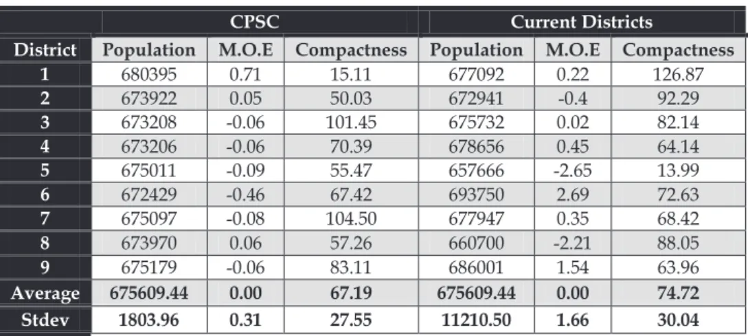
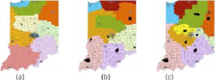
State of Indiana.We further apply our algorithm CPSC to a larger and more complex data set using the census tract data set of the state of Indiana. There are 1,413 polygons (census tracts) in Indiana, and the number of seats assigned to Indiana is nine. Therefore, k¼9 with total expected population of each district equal to 675,610. Fig. 5 presents the districts formed by the graph partitioning algorithm (Fig. 5a), SARA (Fig. 5b), the genetic algorithm for zone design (Fig. 5c), CPSC (Fig. 5d) and the 110th congressional district plan for Indiana (Fig. 5e). Tables 3 and 4 compare the results and it is observed that CPSC produces districts that match the input criteria the most.

Finally, Table 5 shows a runtime comparison of the simulated annealing redistricting algorithm, the genetic algorithm for zone design, and constrained polygonal

spatial clustering algorithm. We observe that while CPSC takes more time than SARA when the number of polygons being clustered is small, the time required by CPSC for a larger data set does increase as fast as it does for the other two algorithms.

In both the experiments described above, CPSC pro-duces clusters that are spatially contiguous, compact, and conform to the other constraints presented to the algorithm as inputs. Furthermore, a visual inspection of Figs. 4 and 5 show us that CPSC produces the most compact clusters, which is further verified by the compactness indices produced using the Schwartzberg index. The comparison of results in Tables 1, 2, 3, and 4 shows us that CPSC is the only algorithm that produces clusters with the most equitable population division within the districts. Further-more, Table 5 lists a runtime comparison of CPSC with the other three techniques. SARA produced the result the fastest (1.9 minutes) with a small data set; however, the plan produced was not optimal. CPSC produces a plan faster (13.41 minutes) than SARA (49.18 minutes) when the data set size almost triples.

The main reason behind CPSC’s superior performance is the use of heuristic function in seed selection, and in deciding which cluster to grow and which polygon to add to the selected cluster. This feature of parallel growth of all

TABLE 1

Comparison of Clustering Results for Nebraska Data Set

TABLE 2

Comparison of Clustering Results for Nebraska Data Set (Contd.)

Fig. 4. Results of (a) Graph Partitioning Algorithm, (b) and (c) SARA: Input (left) and Output (right) plan 1 and 2, (d) the Genetic Algorithm, (e) the CPSC Algorithm, (f) 110th Congressional District Map for the state of Nebraska.

the clusters and unbiased selection of polygons is the novelty of CPSC and makes it better than other redistricting algorithms. Finally, another unique feature of CPSC is the use of the cost function as a part of the heuristic function that measures the reduction in flexibility of clustering with

every assignment of a polygon to a cluster. Thus, for redistricting purposes, CPSC gives an optimal starting plan as opposed to randomized plans produced by other methods.

5.2 Evaluation of Extensions of CPSC

In the next experiment, we used a partial census block data set from the state of Texas to compare CPSC and CPSC*. Basically, we first assumed the constraints were hard when applying CPSC and then assumed that the same constraints could be relaxed when applying CPSC*. This does not imply that in the real district formation problem that constrains could be arbitrarily relaxed. Our goal here was to highlight the impact that CPSC* could have on the redistricting problem if constraints were soft.

TABLE 4

Comparison of Clustering Results for Indiana Data Set (Contd.)

TABLE 5

Runtime Comparison (Minutes) on Intel Pentium Processor T4300, 4 GB Memory

Fig. 5. Results for the Indiana data set. (a) Graph partitioning, (b) SARA, (c) GA, (d) CPSC, and (e) current districts.

TABLE 3

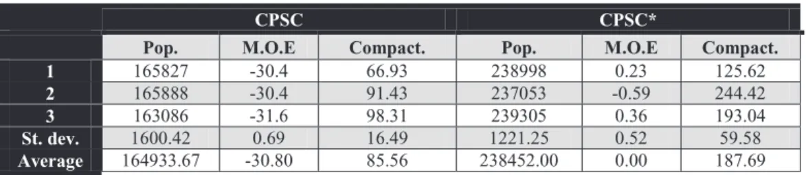
First, we randomly picked three blocks and designated them as school polygons, and setk¼3. The data set consists of 160 polygons (Fig. 6a). The problem statement for the school district formation problem has been described in Section 4.2. The expected result is to seeknumber of school districts. Each school district should have approximately equal number of students, and the farthest household in any district from the school must be within the threshold distance (the maximum distance allowed between a poly-gon and the school polypoly-gon). To begin with, the desired student population within each district is 238,452 with a margin of error of 1 percent, and the desired threshold distance is 10 miles. When CPSC was applied to this data set, all the polygons were not assigned to a cluster because some of the polygons were further away from the school polygon (Fig. 6b). However, as the problem statement dictates that the threshold distance may be relaxed, and thus may be treated as a soft constraint, we applied CPSC* next to this data set. The threshold distance is increased by 5 miles. The result of CPSC* is presented in Fig. 6c. A visual inspection of Fig. 6c shows that every polygon has now been assigned to a cluster. Table 6 lists the population in each district, the margin of error of the population, and the compactness of each district formed by CPSC and CPSC*. In Table 6, none of the districts obtained by CPSC* have a margin of error more than 1 percent.

For the school district experiment, CPSC does not provide a solution for the problem, because an optimal solution does not exist within the data set. That is, all the constraints cannot be satisfied by all the polygons within the data set. This is because, some of the big polygons are farther away from all seed polygons than the maximum distance allowed within a district. However, if the problem is allowed to be modified such that the constraints can be relaxed, i.e., the maximum distance allowed within a district between the seed polygon and any other polygon is increased, then CPSC* is able to provide an optimal solution for the school district problem.

In order to validate CPSC*-PS, we conducted an experi-ment with a synthetic data set that consists of a set of 20 polygons with 1,000 population each (Fig. 7a). The target

is to divide the data set into three clusters with a total population of 6,666 each. When CPSC is applied to this data set, the algorithm does not converge because the target can never be achieved. Once every cluster has achieved a population of 6,000 each, the clusters are stuck fighting for the remaining two polygons. If on the other hand, CPSC* is applied to this data set, and constraint of equal population is converted to a soft constraint of population between 6,000 and 7,000, the result obtained is three clusters with total population 6,000, 7,000, and 7,000, respectively (Fig. 7b). However, as the initial target of 6,666 is not yet achieved, CPSC*-PS is applied next to this data set. Each polygon within the data set is subdivided into two smaller polygons, with the population divided equally within the two smaller polygons. CPSC*-PS when applied to this data set results in three clusters with population 6,500, 6,500, and 7,000, respectively (Fig. 7c).

From these observations, we see the strengths and weaknesses of the CPSC family. CPSC is suitable for situations where the constraints are hard, and a solution exists within the data set. However, if the constraints are soft, and can be prioritized, CPSC* is a better choice than CPSC. CPSC*-PS is the same as CPSC* with the additional step of splitting polygons in order to optimize the clusters discovered with CPSC*. Thus, CPSC*-PS is computationally more expensive than CPSC and CPSC*, and therefore must be used in situations where the polygons can be split into two or more smaller polygons such that the smaller polygons are still meaningful in the context of the

Fig. 6. (a) School district data set (b) CPSC result (c) CPSC* result.

Fig. 7. Application of CPSC* and CPSC*-PS on a synthetic data set. (a) The synthetic data set. (b) Result of CPSC*. (c) Result of CPSC*-PS.

TABLE 6

application. For example, a county can be split into census tracts while forming congressional districts because a census tract is a more compact polygon with smaller population. However, in other applications, e.g., clustering watersheds, splitting a watershed is not meaningful and hence the result obtained by CPSC*-PS is not valid.

5.3 Seed Selection Analysis

In the section, we further analyze the CPSC suite of algorithms in terms of their sensitivity to the initial seeding. One would assume that the seed selection process has an impact on the final results of the algorithm. We conduct an experiment with a synthetic data set where polygons are well defined and uniform, and another with real data polygons to observe how different seed selection processes yield different clusters.

Experiment with synthetic data set. The data set consists of a set of 27 polygons with 1,000 population each, and uniform shape and size. The target is to divide the data set into three clusters with total population of 9,000 each and that each cluster is spatially contiguous and compact. The results with the use of different seed selection functions are presented in Figs. 8a, 8b, and 8c. CPSC produces the same result irrespective of the initial seeds selected. Fig. 8c further demonstrates that CPSC is robust enough to migrate the seeds from their original location such that the clusters satisfy all the user-defined constraints when there is only one optimal solution within the data set. The migration takes place when two or more neighboring clusters compete for polygons. A cluster that has no free neighbor polygons will grab the already-assigned polygons from neighboring clusters in order to continue to grow to meet the target population, while a cluster that has free neighbor polygons will grab the free polygons until it meets the target. Thus, this allows the cluster centers to move apart, as indicated in Fig. 8c.

Experiment with real data set. While the above experi-ment demonstrates the ability of these clusters migrating through space to find the optimal solution, it is very possible that if different clusters have different neighborhoods of free polygons to grow with, it is likely to have multiple clustering solutions. Thus, we experiment with the real-world con-gressional redistricting data set for the state of Indiana. We modify the criteria for the selection of seeds as specified previously in Section 4.1.1. The different seed selections, and the respective congressional districts produced as per the seeds selected are shown in Fig. 9. In Fig. 9a, the seeds are selected by first sorting the census tracts in ascending order of their population and picking the topk¼9polygons that are at least certain distance apart (see (7) in Section 4.1.1) whereas in Fig. 9b the seeds are selected by sorting the seeds in descending order of their population. In Fig. 9c, the seeds are selected by sorting the seeds in descending order of their

populationandwith a smaller distance requirement (i.e., the seeds are allowed to be closer). Briefly, the first strategy is to be conservative when growing clusters by selecting the smallest polygons first, as growing from the smallest polygons first would give each cluster the most flexibility in selecting the next polygons to grow. The second strategy is to grab the largest polygons as seeds and grow them accordingly, with the expectation that each large polygon will serve as the core of a cluster by grabbing neighboring, smaller polygons. The third strategy is similar, but with a reduced requirement allowing seeds to be closer. While all the three seed selection strategies meet the equal population criteria with 1 percent margin of error, we can see that the three results are not the same. This is indicative of the presence of multiple solutions within the data set. Further-more, we can see that the districts in Fig. 9a are the most compact, followed by the districts in Fig. 9b and then those in Fig. 9c. In Fig. 9c, in particular, the reduced distance between the initial seeds causes additional competition for polygons when the clusters grow. Thus, the resulting clusters are more elongated. We thus conclude that

1. the three strategies work as expected,

2. the initial seed selection strategy has an impact on the clustering outcome—as our algorithms are after all order dependent,

3. conservative strategies will yield more compact clusters, and,

4. finally, using initial seeds that are too close together could crowd the growth and cause elongated clusters.

6

C

F

W

In this paper, we have proposed a new spatial clustering approach for polygon data sets instead of point data sets. This approach makes use of the available domain knowl-edge in the form of constraints that guide the clustering process. Our algorithm, called constrained polygonal spatial clustering, views clustering as a search process, with seeds as the start states, and the desired clusters satisfying or optimizing the constraints as the goal states. Thus, it can employ an A search-like mechanism that allows CPSC to embed the constraints into the heuristic function that guides the “search” process. Specifically, CPSC strategically uses constraints to select initial seeds, to compute the distance and cost functions to select the best cluster to grow next, and to select the best polygon to add to the best cluster. While CPSC works with hard constraints, we have developed two extensions of CPSC—namely, CPSC* and CPSC*-PS that work with both hard and soft constraints. We have successfully applied the CPSC algorithm family to two

Fig. 8. Application of CPSC on a synthetic data set. Three initial seeds are

color coded as blue, pink, and green. CPSC results with different seeds. _{Fig. 9. (a) CPSC results with minimum population seeds. (b) CPSC} results with maximum population seeds. (c) CPSC results with maximum population seeds but with smaller distance.

challenging problems: congressional redistricting and school district formation. We have shown that CPSC outperforms other approaches proposed in literature such as simulated annealing and genetic algorithms. In terms of future work, our immediate next step is to apply CPSC*-PS to a real application data set, and perform further evalua-tions of the algorithm, along with developing a parameter-ized heuristic function that allows the user the flexibility to define a set of constraints, and define the constraints as hard or soft. We will then comprehensively evaluate the differ-ences within the algorithms in the CPSC suite, by applying them to solve a real-world problem other than the ones mentioned in this paper. We will also be implementing the congressional redistricting problem more comprehensively by considering additional constraints such as the must-link constraint for minority-population areas, and test the scalability of our algorithm. In addition, we plan to consider other measures for compactness and testing with different cost functions, and see the difference in the clustering results. CPSC may further be benefitted by the use of the spatial characteristics such as topological relationships of the polygons.

A

This material is based upon work supported by the US National Science Foundation (NSF) under Grants Nos. 0219970 and 0535255.

R

[1] M. Altman, “Is Automation the Answer? The Computational Complexity of Automated Redistricting,” Rutgers Computer and Technology Law J.,vol. 23, pp. 81-142, 2001.

[2] F. Bac¸ao, V. Lobo, and M. Painho, “Applying Genetic Algorithms to Zone Design,”Soft Computing,vol. 9, pp. 341-348, 2005.

[3] S. Basu, A. Banerjee, and R.J. Mooney, “Semisupervised Cluster-ing by SeedCluster-ing,”Proc. 19th Int’l Conf. Machine Learning (ICML ’02),

pp. 19-26, 2002.

[4] L.D. Bodin, “A Districting Experiment with a Clustering Algo-rithm,”Democratic Representation and Apportionment: Quantitative Methods, Measures and Criteria,Annals of New York Academy of Sciences, 1973.

[5] D.M. Clayton, African Americans and the Politics of Congressional Redistricting,pp. 138-140. New York Garland Publishing Co., 2000.

[6] I. Davidson and S.S. Ravi, “Clustering with Constraints: Feasi-bility Issues and the K-Means Algorithm,”Proc. SIAM Int’l Conf. Data Mining,2005.

[7] I. Davidson and S.S. Ravi, “Towards Efficient and Improved Hierarchical Clustering with Instance and Cluster Level Con-straints,” technical report, Dept. of Computer Science, Univ. at Albany, 2005.

[8] A. Demiriz, K. Bennett, and M. Embrechts, “Semi-Supervised Clustering Using Genetic Algorithms” Intelligent Engineering Systems through Artificial Neural Networks 9, C.H. Dagli et al., eds., pp. 809-814, ASME Press, 1999.

[9] N. Grira, M. Crucianu, and N. Boujemaa, “Unsupervised and Semi-Supervised Clustering: A Brief Survey,”A Rev. of Machine Learning Techniques for Processing Multimedia Content,Report of the MUSCLE European Network of Excellence (6th Framework Programme), 2005.

[10] J. Han, M. Kamber, and A. Tung, “Spatial Clustering Methods in Data Mining: A Survey,”Geographic Data Mining and Knowledge Discovery,H. Miller and J. Han, eds., vol. 21, Taylor and Francis, 2001.

[11] B. Hayes, “Machine Politics,”Am. Scientist,vol. 84, pp. 522-526, 1996.

[12] M. Halkidi and M. Vazirgiannis, “NPClu: An Approach for Clustering Spatially Extended Objects,” Intelligent Data Analysis

vol. 12, no. 6, pp. 587-606, 2008.

[13] D. Joshi, A.K. Samal, and L.-K. Soh, “Density-Based Clustering of Polygons,”Proc. IEEE Symp. Series on Computational Intelligence and Data Mining,pp. 171-178, 2009.

[14] D. Joshi, L.-K. Soh, and A.K. Samal, “Redistricting Using Heuristic-Based Polygonal Clustering,”Proc. IEEE Int’l Conf. Data Mining,pp. 830-836, 2009.

[15] D. Joshi, A.K. Samal, and L.-K. Soh, “A Dissimilarity Function for Clustering Geospatial Polygons,” Proc. 17th ACM SIGSPATIAL Int’l Conf. Advances in Geographic Information Systems (GIS ’09),

pp. 384-387, 2009.

[16] M.H.C. Law, A. Topchy, and A.K. Jain, “Clustering with Soft and Group Constraints,”Proc. Joint IAPR Int’l Workshop Syntactical and Structural Pattern Recognition and Statistical Pattern Recognition,

2004.

[17] W. Macmillan, “Redistricting in a GIS Environment: An Optimi-zation Algorithm Using Switching Points,”J. Geographical Systems,

vol. 3, pp. 167-180, 2001.

[18] H. Mann and W.B. Fowle,The Common School Journal,pp. 1838-1851. Marsh, Capen, Lyon, and Webb, 1841.

[19] C. Ruiz, M. Spiliopoulou, and E.M. Ruiz, “C-DBSCAN: Density-Based Clustering with Constraints,”Proc. 11th Int’l Conf. Rough Sets, Fuzzy Sets, Data Mining and Granular Computing,pp. 216-223, 2007.

[20] S.J. Russell and P. Norvig, Artificial Intelligence: A Modern Approach,pp. 96-101. Prentice Hall, 2003.

[21] C.-A. Saita and F. Llirbat, “Clustering Multidimensional Extended Objects to Speed Up Execution of Spatial Queries,”Proc. Ninth Int’l Conf. Extending Database Technology (EDBT ’04),pp. 403-421, 2004.

[22] J. Schwartzberg, “Reapportionment, Gerrymanders, and the Notion of Compactness,”Minnesota Law Rev., vol. 50, pp. 443-452, 1996.

[23] K. Wagstaff, C. Cardie, S. Rogers, and S. Schroedl, “Constrained K-Means Clustering with Background Knowledge,”Proc. 18th Int’l Conf. Machine Learning (ICML),pp. 577-584, 2001.

[24] K. Wagstaff and C. Cardie, “Clustering with Instance-Level Constraints,” Proc. 17th Int’l Conf. Machine Learning, pp. 1103-1110, 2000.

Deepti Joshireceived the BA degree in english literature from Delhi University, the MS degree in applied computer science from the Northwest Missouri State University, and the PhD degree in computer science from the University of Nebras-ka in 2011. Her research interests include geospatial computing, data mining, and volun-teered geographic information systems.

Leen-Kiat Soh received the BS (with highest distinction), MS, and PhD (with honors) degrees in electrical engineering from the University of Kansas. He is an associate professor in the Department of Computer Science and Engineering at the University of Nebraska. His primary research interests are in multiagent systems and intelligent agents. He has applied his research to computer-aided education, intelligent decision support, and distributed GIS. He is a member of the IEEE.

Ashok Samal received the bachelor of tech-nology degree in computer science from the Indian Institute of Technology, Kanpur, India, in 1983, and the PhD degree in computer science from the University of Utah, Salt Lake City. He is a professor in the Department of Computer Science and Engineering at the University of Nebraska. His current research interests in-clude geospatial computing, data mining, image analysis, and computer science education. He is a member of the IEEE.