DOTTORATO DI RICERCA IN
FISICA FONDAMENTALE ED APPLICATA
Ciclo: XXVI
Coordinatore: prof. Raffaele Velotta
Study of a Multivariate Technique for the Search of
Single Top-Quark Production with
√
s
= 8
TeV in the CMS
Experiment at CERN
Settore Scientifico Disciplinare FIS/05
Dottorando
Oktay Do˘gang¨un
Tutore
Dr. Luca Lista
Dr. Mario Merola
Contents iii
Introduction 1
I The Theory: Standard Model and Top Quark 5
I.1 The Standard Model . . . 6
I.1.1 Quantum Electrodynamics . . . 8
I.1.2 Electroweak Inteactions and the Higgs Mechanism . . . 11
I.1.3 Strong Interactions . . . 16
I.2 Top Quark . . . 17
I.2.1 Decays. . . 19
I.2.2 Top Quark Production. . . 20
I.2.3 Experimental Results . . . 23
II The Experiment: LHC and CMS 25 II.1 The Large Hadron Collider . . . 26
II.1.1 Design and Layout . . . 28
II.1.2 Magnets . . . 29
II.1.3 Vacuum System . . . 30
II.1.4 RF Acceleration System . . . 31
II.1.5 Accelerator Physics . . . 31
II.2 The Compact Muon Selenoid . . . 33
II.2.1 Detector Design . . . 33
II.2.2 Superconducting Magnets . . . 33
II.2.3 Tracking System . . . 34
II.2.4 Electromagnetic Calorimeter . . . 35
II.2.5 Hadron Calorimeter . . . 36
II.2.6 Forward Detectors . . . 37
II.2.7 Muon System . . . 37
II.2.8 Trigger . . . 38
II.3 Reconstruction . . . 39
II.3.1 Particle Flow Algorithm . . . 39
II.3.2 Tracking Charged Particles . . . 40
II.3.3 Electrons . . . 41
II.3.4 Muons . . . 41
II.3.5 Jet Algorithm. . . 43 iii
II.3.6 Missing Energy . . . 44
III The Analysis: Single Top-Quark Cross-Section Measurement using Multivariate Techniques 45 III.1 Event Selection and Reconstruction. . . 46
III.1.1 Primary Vertex, Noise Cleaning and Triggers . . . 47
III.1.2 Electrons and Muons. . . 47
III.1.3 Jets . . . 48
III.1.4 Missing transverse energy and W-boson transverse mass . . . 49
III.1.5 b-tagging and mistagging . . . 50
III.1.6 Top quark . . . 51
III.2 Control Samples and Data-driven Background Estimations . . . 52
III.2.1 Vector Bosons + jets . . . 52
III.2.2 Top-antitop . . . 52
III.2.3 QCD Background Estimation . . . 53
III.3 Systematic Uncertainties. . . 53
III.3.1 Background Normalisation . . . 54
III.3.2 Instrumental Uncertainties . . . 54
III.3.3 Theoretical Uncertainties . . . 55
III.4 BDT Discriminant . . . 55
III.4.1 Determining Variables . . . 57
III.4.2 Training and Testing . . . 66
III.4.3 Fit Procedure and the Measurement . . . 69
III.5 Results. . . 73 Conclusion 75 Acknowledgements 76 List of Figures 77 List of Tables 79 Bibliography 81
There are two main approaches so far in the human history to understand the nature: reductionism and holism. In a reductionist view, the universe is understood in terms of its pieces, while in the holistic picture, the pieces are understood in terms of the universe itself.
Physics has been using the two approaches in every part of any research. However, one could roughly consider that the physics is actually divided into these points of view in terms of the theories so far, namely the Standard Model of Particle Physics, describing the universe by reducing everything to particles, and the Standard Model of Cosmology, considering the effects of the whole universe on a body of interest.
The physicists have failed to find a theory that describes both the particle physics and the cosmology so far. However, as the experiments and theoretical tools get advanced, the two descriptions would meet at a point where as well as the two approaches start to combine.
This work is presenting a study for the search of the single top-quark production in the CMS Experiment at CERN focusing on thes-channel process and muon decay mode as the final state topology, using a multivariate technique based on the Boosted Decision Trees (BDT) algorithm. The multivariate technique is utilized with an optimization procedure for understanding what are the appropriate variables to use for separation of the signal and background events.
The particle in interest for this analysis, known as top quark, is the heaviest elementary particle predicted by the Standard Model and discovered so far, even heavier than the Higgs boson, discovered in 2012, which itself gives mass to the top quark. It has been discovered after a long survey beginning from the prediction in 1974 by Christenson et al. to the discovery announcement by CDF and DØ in 1994.
Top quark was first postulated in order to dismiss the complications in the established theoretical model of hadrons due to the observation of CP-Violations in kaon decay, followed by Kobayashi and Maskawa who suggested a third generation of quarks to rectify theory and experiment. The additional doublet was called “top” and “bottom” in the spirit of “up” and “down” quarks by Harari who echoed the prediction of a new generation of quarks.
Top quark gives the unique opportunity to perform a direct measurement of the element of the quark-mixing matrix involving the b quark, which is one of the Standard Model parameters. The prompt decay of top quark due to its heavy mass reveals the possibility to investigate the properties of a bare quark before forming any bound state, unlike other quarks known so far.
Beside its importance to the Standard Model, top quark also provides a window for a possible new physics beyond the Standard Model, such as an extra intermediate charged boson W0, fourth generation quarks, charged Higgs boson.
This work is structured in three main chapters:
Chapter I The Theory. The first chapter is presenting the theoretical framework of the top quark physics starting from the Standard Model of particle physics. Af-ter introducing Quantum Electrodynamics, the electroweak and strong inAf-teractions are constructed as an extension of it in a gauge-theoretical manner. Then in the following section, the top quark is detailed considering its decay and its two production mecha-nisms, together with the windows it opens for the feature physics beyond the Standard Model.
Chapter II The Experiment. The second chapter is illustrating the experimental setup detailing the accelerator complex and the detector together with some phenomeno-logical concepts on collider physics. The first section of the second chapter introduces the accelerator complex, the Large Hadron Collider (LHC), while the second section gives a detailed description of the Compact Muon Selenoid (CMS) detector where the data is taken. The third section is about the concepts and physical aspects that the physicists deal with, in the collider phenomenology.
Chapter III The Analysis. The analysis reported in the third chapter is on the collision data collected at 8 TeV in the CMS detector with a luminosity of 19.3 fb−1, focused on muonic decay of the top quark in thes-channel topology. The first section of this chapter is about the event selection used in the analysis while in the second section, the control samples and backgrounds are explained. The third section is about the systematic uncertainties. The fourth section gives a detailed explaination of the analysis using a multivariate technique called the Boosted Decision Trees (BDT) by choosing the most discriminating variables via a feedback loop. The results of the analysis are given in the last section.
The Theory: Standard Model and
Top Quark
Theories in particle physics are formulated as relativistic field theories where the fun-damental entities are fields as a function of space-time, and particles are described as oscillations of these fields. In a subset of field theories the interactions are modeled in terms of an exchange of force carrying fields imposing some symmetries in the theory, called gauge symmetries.
A field theory is described in terms of actions which are functionals of a Lagrangian and can be variated to derive the equations of motions for various fields of the model in subject.
S[φi(x)] =
Z
d4xL(φi(x))
whereL is the Lagrangian density as a function of the fieldsφi(x) and their space-time
derivatives.
A gauge symmetry corresponds to that the laws of physics do not change under some phase change of the fields, requiring an invariance of the form of the Lagrangian under a group of transformations. These transformations form a set that has some basic algebraic properties, i.e., associativity, inversability and having a unit element. The groups having commutativity are called Abelian which physically corresponds to self-interacting gauge fields.
Throughout this chapter, it is used the natural units, namely the convension ~≡c≡1
where ~ = 6.6×10⁻²⁵GeV-s is the reduced Planck constant, c = 3.0×10⁸m/s is the
speed of light and GeV is giga electron volts1. Therefore, the fundamental units can be read as follows, in terms of proton mass which is approximately 1 GeV:
1m = 1.5×10¹⁶GeV−1, 1s = 4.5×1024GeV−1, 1kg = 0.5×1027GeV
This chapter gives a brief introduction to the Standard Model of Particle Physics in terms of fundamental interactions, followed by a detailed section dedicated for the top-quark part of the Standard Model in a phenomenological point of view. Experimental evidence of the Standard Model is given very shortly while recent researches aboout the top quark is listed in the end of the chapter.
I.1
The Standard Model
The Standard Model of Particle Physics is a parametrization of the Quantum Field The-ory where the particles are quantizations of fields interacting according to an algebraic group. More precisely, Standard Model consists of three types of interactions of nature, namely electromagnetic, weak and strong interactions, which are unifiable in the base of the parameters subject to the experiments [2–6].
Each interaction in this picture is described by a symmetry that give rise to a conserva-tion of a quantity in and out of that interacconserva-tion. These symmetries are well understood by some transformations that form an algebraic group, called the gauge group, while the conserved quantity, namely the physical charge, is simply the generator of that group [7,8]. So, the Standard Model is a product of three gauge groups, each corresponds to an interaction, as follows: U(1)Y | {z } hypercharge ⊗ SU(2)L | {z } isospin ⊗ SU(3)C | {z } color charge
where⊗is group product, U(1)Y is the Unitary Group of the hyperchargeY, SU(2)L is
the Special Unitary Group of the isospin T~, and SU(3)C is the Special Unitary Group
of color charge λ. Each group has a fundamental representation which corresponds to
1
1 electron volt is the energy needed for an electron to travel 1 meter under an electrical potential of 1 volt [1].
the particles of the matter like electron or neutrino, and an adjoint representation which corresponds to the force-carrying particles like photon or nuclear force.
The first two symmetries break down simultaneously via the Higgs mechanism [9–12] into a unitary symmetry of the electric charge, Q which is related to the z component of the isospin charge and the hypercharge by the Gell-Mann–Nishijima formula:
U(1)Y ⊗ SU(2)L U(1)Q+ massive bosons
1
2Y + T
3 = Q
After the breakdown, the three gauge bosons of the former groups are eliminated via field redefinitions by the three states of the Higgs field to form massive gauge bosons responsible for the weak nuclear forces, namely the W bosons and the Z boson, so that a massless photon responsible for the electromagnetic force remains and a chargeless Higgs boson becomes observable. The isospin and hypercharge symmetries are indeed broken due to the precence of the masses of the W and Z bosons while the new symmetry of the electrical charge is not since the photon remains completely massless.
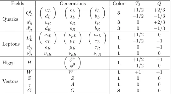
The Standard Model predicts three generation of fermions which consist of two main categories called quarks and leptons (Table I.1). There does not exist a fundamental interaction between quarks and leptons since the color symmetry of SU(3)C is not broken
and leptons are color-singlets while quarks have three types of color charge, so-called “red”, “green” and “blue” 2.
Each fermion has a left-hand and a right-hand helicity, which is defined simply by the contrast between the directions of its spin and the velocity vectors, each having different quantum numbers. Both quarks and leptons form one isospin doublet and two singlet states for each generation. Each isospin doublet hasT = +1 andQ=−1 in total so that it can interact withW±andZ bosons while singlets can not. Especially, the right-hand neutrino singlets, νRi, are completely isolated (or do not even exist) according to the Standard Model, so they do not have any kind of charge. This means that the weak interaction simply breaks the left-right symmetry.
The photon and Z boson are a combination of two parts, each stemming from the isospin group and the hypercharge group, with a mixture angle called the weak angle,θw, which
is just in the exact value that makes the mass of the photon exactly zero, i.e., Mγ = 0. 2
The color charge has nothing to do with physical colors. The names are given so just because there exist three types of conserved quantity for the group SU(3).
Fields Generations Color T3 Q Quarks QiL uL dL cL sL tL bL 3 +1/2 −1/2 +2/3 −1/3 uiR uR cR tR 3 0 +2/3 diR dR sR bR 3 0 −1/3 Leptons LiL νeL eL νµL µL ντ L τL 1 +1/2 −1/2 0 −1 eiR eR µR τR 1 0 −1 νRi νeR νµR ντ R 1 0 0 Higgs H φ+ φ0 1 +1/2 −1/2 +1 0 Vectors W W+ 1 +1 +1 Z Z 1 0 0 γ A 1 0 0 G G 8 0 0
Table I.1: The periodic table of Standard Model. The anti-particles are not included.
Therefore, this parameter of the Standard Model importantly gives the ratio between the mass of the W and Z boson, as follows:
cosθw =
MW
MZ
(I.1)
where it corresponds to sin2θw ≈1/4.
The gluons,G, have eight colors which are a combination of a color and an “anti-color”, so that quarks could interact with the gluons to change their color but not their flavours, isospins or electric charges. The gluons are presumed to be massless since it is not a broken symmetry.
I.1.1 Quantum Electrodynamics
Quantum Electrodynamics (QED), the theory describing the interactions between light and matter, is the first true and successful quantum field theory that was developed [13–17]. All further theories are an extention of the theory to a more general gauge group. Namely, it is the most simple case of a gauge group: the Abelian case, which means that it has no self-interacting terms for the photon as what is observed indeed. QED is the first theory which describes the force as a particle exchange, by explaining the four-fermion interaction of the Fermi theory as a virtual photon exchange between
electrons or positrons. The photons are called virtual because they are observed indi-rectly as a momentum transfer.
The strength of the interaction is precisely given by taking into account high order interactions which is the case in the real world, namely as fine structure constant αe≡
e2/4π≈1/137 is measured to be
αe = 7.297 352 5698(24)×10−3 (I.2)
The Lagrangian of a free massive Dirac field, namely the electron, is written as follows:
L0 = iΨ¯eγµ∂µΨe−meΨ¯eΨe (I.3)
whereγµare the 4×4 Dirac Gamma matrices satisfying the anti-commutation relation,
{γµ, γν}= 2gµν1, (I.4)
and ¯Ψe≡γ0Ψ†is the anti-Dirac spinor, i.e. pozitron, and1denotes the 4×4 unit matrix
in the spinor space. Therefore, the Dirac field Ψe(x) is a 4-component complex column
living in the spin space which means that it has “left” and “right” spin components coupled to each other respectively for electron and its anti-particle pozitron. Thus, a projection operator could be defined in order to seperate the left and right components of the spinor as follows:
PL≡1−γ5, PR≡1+γ5
where γ5 ≡ iγ0γ1γ2γ3. Therefore, the left and right components would be defined as follows, respectively:
eL≡PLΨe, eR≡PRΨe. (I.5)
The left electron has the direction of its spin vector and the momentum vector the same while the right electron corresponds to an opposite case. The mass term of the Dirac Lagrangian would be as the following, after the decomposition to left and right components:
Please note that a mass term for a fermion explicitly breaks the global left-right sym-metry. The Lagrangian for the free photon field, the so-called Maxwell term, is written as follows:
LM0 = −1
4F
µνF
µν (I.7)
where Fµν =∂µAν −∂νAµ is the field strength tensor of the electromagnetic field Aµ.
The total Lagrangian of the Quantum Electrodynamics would be as the following:
LQED = LD0 +LM0 +Lint (I.8)
where the last part is the interaction terms of electron and photon defined as follows
Lint = −iqΨ¯eΨeγµAµ. (I.9)
Here,q is the interaction coupling constant to be determined by the experiments. This is the only possible interaction of a Driac field and a photon since higher order terms would make the theory non-renormalizable, i.e., some integral over momenta of a closed loop in the inetraction woul become divergent in perturbative calculations [18].
Now, one may consider a phase transformation by a arbitrary parameter θ(x) as a function of space-time, as follows:
eL,R 7→eiqθ(x)eL,R, ¯eL,R7→e−iqθ(x)¯eL,R (I.10)
where q is a real number corresponding to the physical electric charge of the fermion, extensively written as q = eQ with ethe electrical constant and Q= −1 for electron. The variance of the free Dirac Lagrangian after this phase transformation would be of the following:
δLD0 = iqΨ¯eΨeγµ∂µθ(x) (I.11)
If one imposes that the total Lagrangian, LQED, should be invariant under the phase transformations, then this implies that the following quantities transform as well:
However, this violates the covariance of the Lagrangian in Eq. (I.8). Therefore, one may redefine a covariant derivative in the Dirac term, as follows:
Dµ ≡ ∂µ−iqAµ (I.13)
This leads the total Lagrangian to be written expicitly as follows:
LQED = i¯eLγµDµeL+me¯eLeR+ h.c.−
1 4F
µνF
µν (I.14)
which is now covariant under an arbitrary phase transformation Eq. (I.10) and Eq. (I.12). This Lagrangian could be extended to any charged fermion like muons, taus, protons, neutrons, etc. instead of only electrons.
I.1.2 Electroweak Inteactions and the Higgs Mechanism
The electromagnetic interaction which describes the dynamics between light and mat-ter, and the weak nuclear interaction which governs the stability of the nucleus are found to be actually originating from a unified interaction in the early universe. This is called Glashow-Weinberg-Salam theory [3–6] of electroweak interactions which includes a mechanism [9–12] that gives masses to the particles, especially to the gauge bosons, via a spinless boson field called the Higgs boson and breaks the symmetry down to QED together with some additional massive bosons responsible for the nuclear forces.
As described in the previous section, QED was an Abelian gauge theory meaning that the gauge boson, i.e. photon, could not interact by itself. On the other hand, the force-carrying bosons of the weak nuclear interaction have a self-inteaction feature, so the gauge group should be non-Abelian.
Considering that the Standard Model includes an SU(2) and an SU(3) gauge groups, first of all it is better to generalize QED discussed in the previous section to a non-Abelian case SU(N). So, one introduces boson fields,Wi, whereiruns from 1 to the number of
generatorsN2−1, and the fermions Ψ, which hasN components in the group space.
where6D≡γµDµ and
Dµ = ∂µ+igTiWiµ (I.16)
is the covariant derivative associated with the generators, Ti. Here Ti are the traceless
unitary generators, which corresponds to the physical charge, of the non-Abelian group withirunning from 1 toN2−1, so that the following gauge transformations leaves the Lagrangian covariant:
Ψ 7→ eigTiθi(x)Ψ (I.17)
Wiµ 7→ Wiµ+∂µθi(x) (I.18)
for a transformation parameter θi(x) as an extension of Eq. (I.10) and Eq. (I.12).
On the other hand, the kinetic term of the bosons is as follows:
LW = −1
4WiµνW
µν
i (I.19)
where
Wiµν = ∂µWiν−∂νWiµ+gfijkWµjWνk (I.20)
and fijk are the structure constants that satisfies the commutation relation of the
gen-erators of SU(N), namely, [Ti, Tj] =fijkTk. Note that the self-interaction terms with
three and four bosons are embedded in this Lagrangian.
In the case of Glashow-Weinberg-Salam theory, the gauge group would be U(1)⊗SU(2). So, there would be two types of gauge bosons, namely, Bµ from U(1) with a single generator called the hypercharge Y and three Wiµ from SU(2) with three generators called the isospinTi fori= 1,2,3.
The masses of the gauge bosons are explained with the Higgs mechanism which describes a spontaneous symmetry breaking because of a spinless self-interacting boson with a non-zero expectation value in the vacuum. Therefore, the so-called Higgs doublet, is defined as follows: H(x) = φ+(x) φ0(x) (I.21)
where the neutral component is decomposed into φ0(x)≡ν+h(x) and
0|φ0|0
= ν (I.22)
is the vacuum expectation value of the Higgs field, with a value of ν ≈ 246 GeV. The reason that the Higgs is a SU(2) doublet is because the Higgs would break the symmetry of SU(2) gauge bosons of which it interacts. So, the non-zero expectation value is stemming from the nature of self-interaction of this field, given in the following Lagrangian: LintH = λ H†H−1 2ν 2 2 (I.23)
where, when expanded explicitly, the term−14λν4 would contribute to the equations of
motion as a constant, while the other terms would consist of a negative squared mass term, −λν2|H|2, and a self-interaction four-vertex, λ|H|4, forλ >0.
The Yukawa interactions, which describes the interaction between a spinless particle and two fermions, reads as follows for the Higgs doublet:
LY = −yijΨ¯iHψj+h.c. (I.24)
where yij is the Yukawa coupling of the fermions, Ψi and ψj which denote a doublet
and a singlet of SU(2), respectively. The Yukawa coupling could be written in terms of the fermion’s mass as mψ
ν so that it would remain a mass term of the fermion for the
vacuum expectation value of the Higgs boson, Eq. (I.22).
Therefore, the full Lagrangian of the Glashow-Weinberg-Salam Model before the sym-metry breaking reads as follows:
LsymmetricEW = iQ¯iL6DQiL+iu¯iR6DuiR+id¯iR6DdiR+iL¯iL6DLiL+ie¯iR6DeiR
−yuijQ¯iLH∗ujR−yijdQ¯iLHdjR−yeijL¯iLHejR+h.c. (I.25) −1 4W µν i W i µν − 1 4B µνB µν+ 1 2(D µH)† DµH−λ |H|2−ν2/2 2
where is a 2×2 anti-symmetric matrix assuring the correct component of the Higgs doublet is contributing, andDµ=∂µ−gTiWµi− 12g
0Y B
µ is the covariant derivative.
the W interaction terms of the kinetic term of the Higgs boson would be diagonalized via changing the fields as follows:
W± ≡ √1
2(W1∓iW2) (I.26)
while the generators would become T±≡ √1
2 T
1±iT2
. The new fieldsW± are called W bosons and they have opposite weak isospin, i.e. T3 =±1 respectively. The corre-sponding charged currents are the following:
Jµ± = QiLγµVijQjL+eiLγµeiL (I.27)
= uiγµPLVijdj+νiγµPLei (I.28)
where Vij is the Cabibbo-Kobayashi-Maskawa (CKM) quark mixing matrix [19, 20].
So, the Lagrangian term embedded in the kinetic energy of the fermions would be as
−√g 2J ± µW µ ±.
Here, the quark mixing is an important aspect for the CP violation observed in nature (e.g. Kaon decays). The CKM mixing is a global U(3) phase rotation in the flavour basis of the quarks interacting with the W boson. This phase transformation leaves the mass of the quarks real-valued and positive while reveals a mixture in the W coupling. So, the CKM matrix is written as follows:
VCKM = Vud Vus Vub Vcd Vcs Vcb Vtd Vts Vtb (I.29)
The parametrization of the matrix has a unremovable complex phase factor which is the only source of the CP violation in the Standard Model.
On the other hand, the remainingW3and Bbosons would mix by an angle of θw, called
the weak angle, as follows:
Z ≡ cosθwW3−sinθwB (I.30)
A ≡ sinθwW3+ cosθwB (I.31)
where e ≡ gcosθw = g0sinθw is the new coupling constant after the mixing, called
interaction: LN Cint = eJµemAµ+ g cosθw Jµ3−sin2θwJµem Zµ (I.32)
where the electromagnetic current and the neutral weak current is defined as
Jµem ≡ X ψ qψψγ¯ µψ (I.33) Jµ3 ≡ X ψ Tψ3ψγ¯ µψ (I.34)
denoting the weak isospin and the electric charge of the fermion ψ by Tψ3 and qψ ≡
T3+ 12Y, respectively, as a result of the redefinitions, Eq. (I.30) and Eq. (I.33). See TableI.1for the values of these charges.
After the symmetry breaking via the Higgs mechanism, the Lagrangian in Eq. (I.25) becomes as follows:
LbrokenEW = iQ¯iL6DQiL+iu¯iR6DuiR+id¯iR6DdiR+iL¯iL6DLiL+i¯eiR6DeiR
−yuiju¯iLhujR−ydijd¯iLhdjR−yeije¯iLhejR+h.c. −miuu¯iLuiR−midd¯iLdiR−miee¯iLeiR+h.c. −1 2W +µν i W − µν− 1 4A µνA µν− 1 4Z µνZ µν (I.35) +1 2∂ µh∂ µh+m2Hh2− gm2 H 4mWh 3− g2m2 H 32m2 W h4 + gmWh+ g2 4 h 2 Wµ−W+µ+2 cos12θ wZµZ µ
−igh(Wµν+W−µ−W+µWµν−)(Aνsinθw−Zνcosθw)
+Wν−Wµ+(Aµνsinθw−Zµνcosθw) i −g 2 4 ( h 2Wµ+W−µ+ (AµsinθW −ZµcosθW)2 i2 −hWµ+Wν−+Wν+Wµ−
+(AµsinθW −ZµcosθW)(AνsinθW −ZνcosθW)
i2 )
where the first line is the kinetic terms with gauge couplings, the second line is the Higgs-fermion couplings, the third line is fermion mass terms, the fourth line is the gauge kinetic terms, the fifth line is the Higgs kinetic energy, mass and self-couplings, the sixth line is the boson-Higgs couplings, the rest of the lines are gauge-gauge couplings.
I.1.3 Strong Interactions
Quantum Chromodynamics (QCD) is the field theory of the strong interactions in an elementary level, i.e. the interaction between quarks (QiL,uiR, diR), and gluons (Gaµ).
Since it is a SU(3) gauge theory, the Lagrangian for QCD-only inetractions could be expressed as follows: LQCD = gsQ¯iLλaGaµQiL+gsu¯iRλaGaµuiR+gsd¯iRλaGaµdiR− 1 4G µν a Gaµν (I.36)
where only the contribution to the covariant derivative for gluon interaction (i.e.,−igsλaGaµ,
see Eq. (I.16)) is written, and the field strength tensor of the gluons,Ga
µν, is in the same
form with Eq. (I.20) with the corresponding generators, λa, and the strong coupling
constant, gs.
The gluons have 8 different colors. These are generated by the 3×3 matrices, called Gell-mann matrices, λa as a color and an anti-color combined in each gluon. In a group
theoretical expression,
3⊗¯3=8⊕1 (I.37)
where3and ¯3stand for color and anti-color triplet,1means a color singlet and8means color octet. The color singlet state, sometimes called the ninth gluon, is not present in the group SU(3), and therefore in the Standard Model, since it is a unit matrix and physically insignificant.
Each (anti)quark is component of a (anti)color triplet labeled as “red”, “green” or “blue” as in the following example:
urediL = ψiL 0 0 ugreeniL = 0 ψiL 0 ublueiL = 0 0 ψiL (I.38)
On the other hand, gluons are spanned by 3×3 Gell-mann matrices, so that the quarks having the appropriate color charges would interact with that gluon. So, each component
of the octet, Gµ≡λaGaµ, reads explicitly as follows: Grgµ = 0 G1µ 0 G1µ 0 0 0 0 0 Ggrµ = 0 −iG2 µ 0 iG2µ 0 0 0 0 0 Grrµ = G3 µ 0 0 0 −G3 µ 0 0 0 0 Grbµ = 0 0 G4 µ 0 0 0 G4 µ 0 0 (I.39) Gbrµ = 0 0 −iG5 µ 0 0 0 iG5µ 0 0 Gbgµ = 0 0 0 0 0 G6µ 0 G6µ 0 Ggbµ = 0 0 0 0 0 −iG7 µ 0 iG7µ 0 Grgbµ = 1 √ 3G 8 µ 0 0 0 √1 3G 8 µ 0 0 0 −√2 3G 8 µ
Note that the QCD Lagrangian, Eq. (I.36), and the EW Lagrangian, Eq. (I.25) or Eq. (I.35), are indeed discrete since in each definition the covariant derivatives were given accordingly, so that the SM Lagrangian could be written as a sum of the two, as follows:
LSM = LQCD+LEW (I.40)
I.2
Top Quark
The top quark, together with the bottom quark, theoretically predicted in 1973 by T. Maskawa and M. Kobayashi to explain the Charge-Parity (CP) violation in Kaon decay, extending the Cabbibo quark-mixing matrix to a three-generation quark-mixing matrix, now called the Cabbibo-Kobayashi-Maskawa (CKM) matrix. Then, the top quark discovered in 1995 by the DØ and CDF experiments at FermiLab.
The top quark is the heaviest particle that is known so far, and as well as among other Standard Model particles, with a mass of 173 GeV. The electrical charge isQt= +2/3,
having an hypercharge of Y = 4/3 (or 1/3) and a weak isospin of T3 = 0 (or 1/2) for
the right (or left) component. The Higgs coupling of top quark is around 0.7 which is the largest among other fermions.
The top quark has a special place in the Standard Model of particle physics and plays a promising role to extend the current boundaries to the new physics. The following considerations of the top quark reveals the search for new physics:
• The top quark is the heaviest particle, which also means that it has the strongest Yukawa coupling among the fermions of the Standard Model. This is promising for seeking new strong dynamics since it is directly related to the breaking of the electroweak symmetry.
• The loop corrections to the Higgs boson mass includes a top quark loop which opens a window to the tera-scale physics, e.g. SUSY, Little Higgs models.
• The rapid decay of the top quark gives a unique route to investigate the nature of a “bare quark” related to its mass, charge and spin.
• The decays of top quark to the heavy states like W, Z or Higgs boson plus a quark have a very large phase space due the high top mass.
• The coupling of the top quark with the W boson offers an opportunity to explore the models beyond the three-generation quarks by directly measuring the CKM mixing matrix element.
The top-quark part of the Standard Model Lagrangian, Eq. (I.40), reads explicitly as follows: LSM,top = itγ¯ µ∂µt Propagation − mttt¯ mass term − mt v ¯tHt Higgs coupling + gs¯tγµλaGaµt gluon coupling + etγ¯ µQA µt photon coupling + cosgθ wtγ¯ µ g V +gAγ5 Zµt Z-boson coupling + √g 2 d,s,b X q
Vtq¯tγµPLWµ−q+ h.c. CKM-mixed W-boson coupling
(I.41)
where gV = 12T3−Qsin2θw and gA=−12T3 are the vectoral and axial couplings to Z
Considering the radiative one-loop corrections to the W boson mass, the top mass con-tributes significantly together with the Higgs boson mass:
m2W = √ πα
2GFsin2θw(1−∆r)
(I.42)
whereGF is the Fermi constant and the correction is calculated as follows:
∆r = − 3GFm 2 t 8√2π2tan2θ w +3GFM 2 W 8√2π2 lnM 2 H MZ2 − 5 6 (I.43)
Therefore, one could reveal a relation between the top mass and the Higgs mass for the given W and Z masses.
I.2.1 Decays
In the Standard Model, top quark decays only via weak interaction to a W boson and a down-type quark, dominantly a b quark. The full decay rate for the top quark is calculated as follows: Γ t→W+q = |Vtq| 2m3 t 16πν2 1 + 2M 2 W m2 t 1 −MW2 m2 t 2 1− αs(4π2−15) 9π (I.44)
where αs is the fine structure constant of the strong interactions. The branching ratio
for theW bdecay is directly related to the CKM mixing parameter as follows:
B(t→W b) B(t→W q) = |Vtb|2 |Vtb|2+|V ts|2+|Vtd|2 (I.45)
which is measured to be 0.91±0.04, means that approximately the 90% of the top quarks decays into a b quark. Since the Standart Model predicts 3 generation of quarks, the constraint |Vtb|2 +|V
ts|2 +|Vtd|2 = 1 might be considered for precise measurements of
the CKM matrix element |Vtb|. On the other hand, without the assumption of
three-generation quarks, the ratio opens a window for extra-three-generation quarks directly. An important aspect of the decay rate given above is that the top quark decays so promptly even before hadronization because the value of the decay rate is greater than the QCD threshold:
where ΛQCD ≈ 250 MeV. This also implies that the lifetime of the top quark is 0.5×
10−24s which is long before the colorless boundstates can form or even before moving away from the interaction vertex into the detector. So, the top quark, as the only known particle to decay before hadronization, gives the unique opportunity to understand the properties of a “bare quark”.
The top quark events are categorized according to the decay modes of the W boson stemming from the top quark because the W boson has a short lifetime, approximately 3×10⁻²⁵s, and this means it can not be directly measured in the detectors. Instead the decay products of the W boson should be studied to understand the top quark events. W boson decays mostly into two quarks which are hadronized to produce jets which is a shower of variety of hadrons might be stopped in the calorimeters of the detector. This decay mode is called “hadronic top decay” and it is hard to separate since there would be a large number of background events with very similar jet topologies. Another decay mode is “leptonic top decay” which means the W boson produces a charged lepton and its associated neutrino. It is called “electron (muon) channel” when the lepton in subject is electron (muon).
I.2.2 Top Quark Production
There are two ways to produce top quark in proton-proton collisions, one via charged-current electroweak interactions as a single, and another via strong interactions as a pair. For this reason, the single top-quark production allows to probe the electroweak sector of the Standard Model with top-quark physics.
Pair production
The top-pair production is either a quark-antiquark anhillation, qq¯→ t¯t, or a gluon fusion, gg → t¯t. An event where the both W bosons decay into quarks is called “fully hadronic” while one or two of theW bosons decay into leptons are called “semi-leptonic” or “di-leptonic”, respectively.
Since hadronic collisions have the hard process via the interaction of the constitutent quarks and gluons which are called partons, the total cross-section of the pair production at a center of mass energy√scould be expressed as a convolution of two contributions.
One contribution is the short-distance interaction between the participating partons at the center of mass energy√sˆ, while the other contribution comes from the long-distance factors that specify the probability density of observing these partons with a certain fraction in the momenta of the incoming hadrons, as follows:
σpp→t¯t = q,q,g¯ X i,j Z dxidxjfi xi, µ2F fj xj, µ2F | {z } long-distance σij→t¯t(xi, xj) | {z } short-distance (I.47)
wherexi is the hadron longitudinal momentum fraction carried by the parton irunning
for all quarks, anti-quarks and gluons, µ2F is the factorization scale, fi(xi, µ2) are the
Parton Distribution Functions (PDFs) of the proton, which is simply the probability density to observe a parton i with the momenta fraction xi such that ˆs = xixjs, and
σij→t¯t is the cross-section of the hard process of the partons producing the top pair.
The hard process, which involves only high momentum transfer and almost insensitive to low momentum scale, is calculable with perturbative QCD. The factorization is valid to all orders of the perturbative theory, getting weaker dependence on the arbitrary scale µ2F as more perturbative terms are added in the expansion. On the other hand, the PDFs characterizing the long-distance process can not be calculated in perturbative QCD, instead are extracted by global fits from deep-inelastic scattering and other data. The minimum ˆs= xixjs in the process is 4m2t and therefore xixj ≥4m2t/s which will
typically be near the threshold for the t¯t production since the probability of finding a parton with fraction x decrease with increasing x. This means that hxi ≈ √xixj ≈
2mt/
√
swould be 0.18 at TeVatron and 0.25 at the LHC, and explains why we observe a dominance of the quark-antiquark annhilation with 85% at TeVatron, but on the other hand, the gluon fusion with 90% at LHC.
The cross-sections calculated for 7, 8, 13 and 14 TeV collision energies are presented in TableI.2.
Cross-Section (pb) 7 TeV 8 TeV 13 TeV 14 TeV
σpp→t¯t 174+11−12 248+14−15 810+38−36 957+44−41
Table I.2: Table of the Standard Model predictions for the top-pair production
Single Production
Three different mechanisms for single top-quark production are predicted in the SM in hadron-hadron collisions according to the virtuality of the W boson (FigureI.1):
• s-channel production asq2>0.
• W-associated, or tW production as q2 =m2W.
• t-channel production asq2 <0.
Figure I.1: The single top-quark production in s-channel (left), W-associated
t-channel (middle) andt-channel (right).
All three channels are directly related to the CKM matrix element|Vtb|, providing the chance for a direct measurement of this SM quantity. There is a special interest in LHC for s-channel single-top production since it is very sensitive to several models of new physics involving fourth-generation quarks, a non-SM mediator, like W0 or a charged Higgs boson.
Cross-Sections (pb) 7 TeV 8 TeV 13 TeV 14 TeV
t-channel 65.9+2−1..68 87.2−+32..4244 219.1+6−3..79 243+8−6
tW-channel 15.6±1.17 22.2±1.52 58.5+2−3..41 83.6+3−5..62
s-channel 4.56−+00..1918 5.55±0.22 10.22+0−0..2221 11.92+0−0..4953
Table I.3: Table of the Standard Model predictions for the single top production
cross-sections for all three production channels at NNLO [22–26].
According to the cross-section calculations of the single-top production as shown in TableI.3, thet-channel searches will benefit mostly in the LHC Run II which will have 13 and 14 TeV collision energies.
I.2.3 Experimental Results
All the measurements done so far are in an agreement with the Standard Model pre-dictions listed in Table I.3. The finalized experiments CDF and D0 Collaborations at Tevatron with 1.96 TeV center-of-mass energy and the current experiments ATLAS and CMS Collaborations at CERN with 7 TeV and 8 TeV center-of-mass energies have reported several results given below.
Observation of single top-quark production was published by the CDF [27–29] and D0 [30,31] collaborations in the sum of the s- and the t-channels. Subsequently, The CDF collaboration reported a measurement of single top-quark production cross-section for the sum ofs-,t-, andW t-channels as 3.04+0−0..5753pb using data corresponding to 7.5 fb−1of integrated luminosity [32] and for the sum of thes- andt- channels as 3.02+0−0..4948pb using up to 9.5 fb−1 of integrated luminosity [33]. The D0 collaboration obtained a cross-section of 4.11+0−0..6055 pb using data corresponding to 9.7 fb−1 of integrated luminosity [34].
The cross sections for each production mode were also measured separately. The D0 collaboration measured the cross-section of the t-channel process to be 3.07+0−0..5449 pb using data corresponding to 9.7 fb−1 of integrated luminosity [34, 35]. On the other hand, the CDF collaboration measured t- and tW-channels as 1.66+0−0..5347 pb using data corresponding to 7.5 fb−1 of integrated luminosity [32] and t-channel as 1.65+0−0..3836 pb using up to 9.5 fb−1 [33] of integrated luminosity. Furthermore, CDF and D0 combined their results [36–38] to observe the s-channel process with 1.29+0−0..2624 pb [38].
At the LHC proton-proton collider,t-channel production at 7 TeV center-of-mass energy was observed to be 84+20−19 pb by the ATLAS collaboration [39, 40] and 83.6±30.0 pb by the CMS collaboration [41]. The 8 TeV measurements in t-channel was reported as 95±18 pb by ATLAS [42] and 80.1+12−7.0.3 pb by CMS collaborations [43]. Furthermore, ATLAS has found evidence for W t-channel production [44], followed recently by an observation at the CMS experiment[45, 46]. The s-channel at √s = 8 TeV in ATLAS has been measured to be 5.0±4.3 pb [47] and in the CMS to be 6.2+8−5..01 pb which is also presented in this work [48]. The CKM matrix element|Vtb|is extracted as 0.998±0.041 at√s= 7 TeV [49].
The Experiment: LHC and CMS
The Lagrangian describes the interactions of a field theory as discussed in Sec. I.1. On the other hand the experiments attempt to measure the rate at which a specified interaction occurs. The bridge between a field theory and experiment is the cross-section for the interaction in subject, which gives the expected number of the events, N, that will result from the collision of a large number of particles.
The cross-section, σ, may be calculated from the Lagrangian using the method of the field theory to produce a prediction that might be tested at a collider experiment such as LHC. The number of events, N, for a specified interaction, namely the “signal”, is given by the following:
Nsignal = σsignalε
Z
dtL (II.1)
where ε is the efficiency of the detector, L is the luminosity, which is defined as the number of particles per unit area per second in the colliding beams, and σsig is the
cross-section. Here the luminosity is integrated over time so that it gives the total number of interactions occured. The cross-section is in units of area, namely “barn”, which is defined as 1b = 10−28m2, tipically measured in femtobarns (fb) or picobarns
(pb) in high energy physics. Therefore the integrated luminosity is in the units of inverse area, tipically given in pb−1 or fb−1 for LHC experiments.
II.1
The Large Hadron Collider
The Large Hadron Collider (LHC) at the European Centre for Nuclear Research (CERN) is a two-ring superconducting proton-proton collider situated in the 27 km tunnel pre-viously constructed for the Large Electron-Positron collider (LEP) [50, 51]. The first beam operation was launched in 2008 with a design to provide proton-proton collisions with a luminosity of 1034cm−2s−1 and a unprecedented centre-of-mass energy of 14 TeV
for the study of rare events, such as the production of the Higgs particle which was observed recently in 2012.
The LHC has two general purpose experiments ATLAS and CMS, aiming to collect data with high luminosity, and two experiments, LHCb for B-physics and TOTEM for the detection of protons from elastic scattering at small angles, working at lower luminosities of 1032cm−2s−1 and 1029cm−2s−1, respectively. In addition to proton-proton operation, the LHC is able to collide heavy nuclei, Pb-Pb, with a total centre-of-mass energy of 1150 TeV which corresponds to 2.76 TeV per nucleon, and for this it has one dedicated ion experiment, ALICE, aiming at a peak luminosity of 1027cm−2s−1.
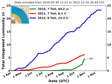
The LHC is decided to be operated at the reduced beam energy of 3.5 TeV for the first two years after an accident occured in 19 September 2008, just 9 days after the very first beam, which caused substantial damage to the magnets and to the beam pipe imposed an intervention of repairs and improvements. Following the pilot runs at 0.9 and 2.36 TeV collision energies, LHC performed the first collision at 7 TeV on 30 March 2010, initially at a low luminosity of about 1×1027cm−2s−1 to reach immediately to a luminosity of 3.6×1033cm−2s−1 in October 2010. The integrated luminosity was recorded by experiments as 44pb−1in 2010, 6fb−1in 2011, and 23fb−1in 2012, as shown in Figure II.1.
The LHC simultaneously accelerates two proton (or lead) beams circulating in opposite directions, so the magnets use a twin bore design to bend particles in both beams simultaneously. There are eight crossing points around the ring where beams can be crossed together to produce collisions, although only four of these are currently in use by LHC experiments.
Protons are initially produced in a duoplasmatron source where electrons that are emit-ted from a cathode filament hit gaseous hydrogen atoms. Then the protons pass through a chain of accelerators starting from the injection into the linear accelerator Linac2 to
1 Apr 1 May 1 Jun 1 Jul 1 Aug 1 Sep 1 Oct 1 Nov 1 Dec Date (UTC) 0 5 10 15 20 25 T o ta l In te g ra te d L u m in o s it y ( fb ¡ 1) £ 100
Data included from 2010-03-30 11:21 to 2012-12-16 20:49 UTC
2010, 7 TeV, 44.2 pb¡1 2011, 7 TeV, 6.1 fb¡1 2012, 8 TeV, 23.3 fb¡1 0 5 10 15 20 25 CMS Integrated Luminosity, pp
Figure II.1: The total integrated luminosity recorded by the CMS experiment in
2010, 2011 and 2012.
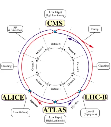
Figure II.2: The LHC injection complex.
reach a preliminary energy of 50 MeV. Then the Proton Synchrotron Booster takes the protons to 1.4 GeV and passes them to the Proton Synchrotron where they are accele-rated to 25 GeV. Before they enter into the LHC in the final stage, the Super Proton Synchrotron, the protons reach 450 GeV.
On the other side, lead ions are formed in an Electron Cyclotron Resonance and later accelerated in Linac3. After they are accelerated in the Low Energy Ion Ring, they are passed to Proton Synchrotron Booster where the protons accelerated as well. So, the remaining stages follow the same as the proton beam as shown schematically in Figure
II.2.
After the two rings are filled, the machine is ramped to its nominal energy of 7 TeV over about 28 min. In order to reach this energy, the dipole field must reach the level for accelerator magnets of 8.3 T. This high field can only be achieved using the super-conducting material NbTi, by cooling the magnets in superfluid helium at a tempreture lower than 2K.
II.1.1 Design and Layout
The basic layout of the LHC follows the LEP tunnel geometry and is shown in Figure
II.3. The machine has eight arcs and straight sections, the last being approximately 528m long. Four of the straight sections house the LHC detectors while the other four are used for machine utilities, radio frequency and collimation systems, and beam dump insertions. The two high luminosity detectors are located at diametrically opposite straight sections. The ATLAS detector is located at point 1 and CMS at point 5, which also incorporates the small angle scattering experiment TOTEM. Two more detectors are located at point 2 (ALICE ) and at point 8 (LHCb), which also contain the injection systems for the two rings. The beams only cross from one ring to the other at these four locations.
The number of events taking place per second at the LHC interaction point is given by
N = σL (II.2)
where σ is the cross-section of the process in subject and L is the luminosity which is expressed as the following:
L = nbn1n2frev
2πΣxΣy
F γr
whereγr is the relativistic gamma factor,F is the geometric luminosity reduction factor
due to the crossing angle at the interaction point, nb is the number of bunches per
Figure II.3: The LHC layout.
and the factors Σx,y represent the horizontal and the vertical convolved beam widths,
respectively. When the machine reaches the desinged peak luminosity of 1034cm−2s−1 for the detectors CMS and ATLAS, the number of particles per bunch would reach
n1,2= 1.15×10¹¹while the number of bunches per beam would be 2808 with a revolution
frequency of 11245 Hz.
II.1.2 Magnets
The LHC contains more than 7000 superconducting magnets ranging from the 15m long main dipoles to the 10 cm octupole/decapole correctors inside the dipole cold masses as well as more than 100 conventional warm magnets and the about 500 conventional
magnets in the two 2.6 km long transfer lines between the SPS and the LHC . The LHC magnet system, while still making use of the well-proven technology based on NbTi Rutherford cables, cools the magnets to a temperature of 1.8 K, using superfluid helium, and operates at fields above 8 T. This so low temperature with respect, for example, to the other large superconducting accelerators, Tevatron, HERA and RHIC which cools the magnets down to 4.5 K, brings a decrease of the heat capacity of the superconductor by an order of magnitude, making the magnets more sensitive to quenches.
Figure II.4: The LHC dipole cross-section [52].
II.1.3 Vacuum System
The design of the beam vacuum system takes into account the requirements of 1.9 K operation and the need to shield the cryogenic system from heat sources, as well as the usual constraints set by chamber impedances. The main heat sources are the synchrotron light radiated by the beam, the image currents, the development of electron clouds and the energy loss by nuclear scattering. Intercepting these heat sources at a temperature above 1.9 K has necessitated the introduction of a beam screen cooled to between 5 and 20 K. This beam screen is perforated in about 4% of the surface area to allow the cold bore of the magnets at 1.9K to act as a distributed cryopump. The slots in the beam
screen are displaced in a pseudorandom pattern to avoid periodic perturbations which can induce resonant beam modes.
II.1.4 RF Acceleration System
The RF system is located at point 4. Two independent sets of cavities operating at 400 MHz (twice the frequency of the SPS injector) allow independent control of the two beams. The superconducting cavities are made from copper whose internal surface is sputtered with a thin film of a few microns of niobium. In order to combat the intrabeam scattering (see below), each RF system must provide 16 MV during coast while at injection 8 MV is needed. Although the RF hardware required is much smaller than LEP due to the very small synchrotron radiation power loss, the real challenges are in controlling beam loading and RF noise.
II.1.5 Accelerator Physics
Here, some effects of the issues in the accelerator physics on the machine is presented briefly.
Coherent instabilities
The interaction of the beam with its environment generates electromagnetic fields which can react back on the beam and drive it unstable. The first step is to design the vacuum chamber to reduce this coupling as much as possible, for instance reducing the resistivity of the copper in the beam screen by cooling it to between 5 and 20 K, or making the chamber smooth without discontinuities.
Nevertheless reducing the resistivity of the environment can reduce but not definitely avoid the growth of the instabilities. The two main instabilities to be kept under control are the transverse coupled bunch instability and the single bunch head-tail instability. Without giving too much detail, the former is due to image currents in the beam screen and its main unstable modes are damped through the action of a pair of electrostatic deflectors. The latter, head-tail effect, is an instability due to the short range wakefields acting between the tail and the head of the bunch. It is taken under control by the action of sextupoles integrated into the short straight sections.
Finally, the Landau damping, which acts on very high frequency oscillation modes, is provided with two families of strong octupoles without need for feedback and, for this reason, it is particularly important when the transverse feedback system has noise problems.
Dynamic aperture
In superconducting magnets of the type used in the LHC, the field quality is determined by the precision of the positioning of the superconductor. It has been shown that the aperture inside which particles orbits are stable, is much smaller than the physical aperture of the beam pipe. It is called dynamic aperture and is limited mainly by the unwanted higher field harmonics due to magnet imperfections. Although sophisticated computer simulations take into account these effects, it is not possible to perform the full scale simulation over 4×10⁷ turns, which correspond to 1 h of storage time. So, in order to insure a dynamic aperture of 6 sigmas, it has been decided to use the tracked dynamic aperture evaluated over 106 turns multiplied by a factor of 2.
The beam-beam interaction
The maximum particle density per bunch is limited by the nonlinear beam-beam inter-action that each particle experiences when the bunches of both beams collide with each other. It reveals a variation of the tune with amplitude, and the excitation of nonlinear resonances due to the periodic nature of the force. The linear tune shift can be expressed by:
ζ = nbrp
4πn
(II.3)
where nb is the number of bunches per beam, n is the normalized transverse beam
emittance,rp is the classical proton radius given byrp =e2/4π0mpc2 in which eis the
electron charge, 0 is the electric permeability and mp is the proton mass. Experience
with hadron colliders indicates that the total linear tune shift summed over all interaction points should not exceed 0.015, and in the LHC case, the tune shift must be ζ <0.005. The long range beam-beam interactions between successive bunches are also reduced by colliding the beams with a small crossing angle of about 400µrad.
II.2
The Compact Muon Selenoid
The Compact Muon Solenoid (CMS ) detector is a multi-purpose apparatus operating at the Large Hadron Collider at CERN [53]. The total proton-proton cross-section at
√
s= 14 TeV is expected to be roughly 100 mb. At design luminosity the general-purpose detectors will therefore observe an event rate of approximately 109 inelastic events / s, leading to a number of formidable experimental challenges. The online event selection (trigger) must reduce the huge rate to about 100 events / s for storage and analysis. Furthermore, at design luminosity we expect a mean of about 20 inelastic collisions per bunch crossing and so around 1000 charged particles will emerge from the interaction region every 25 ns (time between two successive bunch crossing). The superimposition of other events on the event of interest, the so called pile-up effect, can be reduced by using high granularity detectors with good time resolution and low occupancy. This would inevitably require the use of millions of detector electronic channels which need very good synchronization.
II.2.1 Detector Design
The detector design and layout 2.7 is mainly driven by the choice of the magnetic field configuration, needing for large bending power to precisely measure high energy particles momentum. The heart of CMS detector is the big 4 T superconducting solenoid which accommodates the inner tracker and calorimetry inside and is situated immediately before the muon detectors.
II.2.2 Superconducting Magnets
The CMS superconducting solenoid 2.10 has been designed to reach a 4 T field in a free bore of 6 m diameter and 12.5 m length with a stored energy of 2.6 GJ at full current. The flux is returned through a 10000-t yoke containing 5 wheels and 2 endcaps. The distinctive feature of the 1.8 K, 220-t cold mass is the 4-layer winding made from a stabilized reinforced NbTi conductor, needed to be able to reach the desired 4 T magnetic field. The ratio between stored energy and cold mass is high as 11.6 KJ/kg, causing a large mechanical deformation of 0.15% during energizing.
Figure II.5: The design of the Compact Muon Selenoid.
II.2.3 Tracking System
The inner tracking system of CMS is designed to provide a precise and efficient mea-surement of the trajectories of charged particles coming from the LHC collisions, as well as a precise reconstruction of secondary vertices [54]. The tracker which is fully covered by the solenoid magnetic field surrounds the interaction region and has a length of 5.8 m and a diameter of 2.5 m. The high rate of interactions requires high granularity and fast response as well as efficient cooling system and radiation hardness, aspects which led to the silicon technology choice.
The pixel detector in the inner part contains three barrel layers at radii of 4.4, 7.3, and 10.2 cm, respectively, with a length of 53 cm each. The two endcaps for each side are located at |z|= 34.5 cm and|z|= 46.5 cm and extend inr from 6 to 15 cm. The pixel size is 100×150µm2. The strip detector is divided into an inner part and outer part, both divided further into the barrel part and discs that cover the forward region which are called Tracker Inner Barrel (TIB), Tracker Inner Disks (TID), Tracker Outer Barrel (TOB), and Tracker Endcaps (TEC), as shown in Figure II.6.
Figure II.6: The tracker system.
II.2.4 Electromagnetic Calorimeter
The electromagnetic calorimeter of CMS (ECAL) is a hermetic homogeneous calorimeter made of 61200 lead tungstate crystals, PbWO4, mounted in the central barrel part, 7324
crystals in each of the two endcaps and a preshower detector placed in front of the endcap crystals, mainly for π0 identification [55]. Avalanche photodiodes (APDs) are used as photodetectors in the barrel and vacuum phototriodes (VPTs) in the endcaps. The high density of crystals give the calorimeter the characteristics of fast response, fine granularity and radiation resistance, as well as a good capability to detect the decay to two photons of the postulated Higgs boson.
Figure II.7: The hadron calorimeter (HCAL). ECAL and trackers also appear at the innermost part.
It consists of 36 supermodules spanning half of the barrel in z direction and 20◦ in azimuthal direction. The crystals almost point to the nominal interaction point at the center of the detector only by 3◦ in order to avoid particle trajectories coinciding with the boundary between two crystals, as shown in Figure II.7.
II.2.5 Hadron Calorimeter
The hadron calorimeters (HCAL) are particular for the measurement of hadron jets and neutrinos or exotic particles resulting in apparent missing transverse energy [56]. The absorber material is brass which has a reasonably short radiation length, is easy to process and non-magnetic. The active material consists of plastic scintillators read out with wavelength-shifting fibers.
Figure II.8: The hadronic calorimeter (HCAL).
The Hadron Barrel (HB) comprises the pseudo-rapidity range up to ±1.4, extending radially from 1.806 m to 2.95 m. On the other hand, the Hadron Endcaps (HE) includes 14 pseudo-rapidity segments each, covering the region 1.3 ¡|η|¡ 3.0. The Hadron Outer (HO) is placed outside of the solenoid, covering the pseudo-rapidity region±1.26. The Hadron Forward (HF) calorimeter measures hadrons in the forward region and covers a substantial pseudorapidity range of|η|between 3.0 and 5.0, which is important for the measurement of missing transverse energy.
II.2.6 Forward Detectors
The CASTOR (Centauro And STrange Object Research) detector is a quartz-tungsten sampling calorimeter, with characteristics of radiation hardness, fast response and com-pact dimensions, designed for the very forward rapidity region in heavy ion and proton-proton collisions at the LHC. Its physics motivation is to complement the nucleus-nucleus physics program and also to study the diffractive and low-x physics in pp collisions.
II.2.7 Muon System
Muon detection is a very important tool to recognize signatures of interesting pro-cesses over the very high background rate expected at the LHC with full luminosity. An example can be the Standard Model Higgs boson decay in the full leptonic channel
H →ZZ (orZZ?) → 4`, which, in case the leptons are muons, is called “gold plated” channel; or the large variety of Beyond Standard Model theories which predict the presence of muons among the final states. So, precise and robust muon measurement has been a central theme since from CMS earliest design stages.
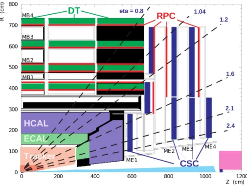
Figure II.9: The muon system of the CMS detector.
Three types of gas detectors are used: Drift Tubes (DT), Resistive Plate Chambers (RPC), and Cathode Strip Chambers (CSC), as shown in Figure II.9. Drift tubes are
used in the barrel region, roughly covering |η|<1.3, where the particle flux is relatively low. The drift tubes are arranged in chambers MB1 to MB4 at radii of about 4.0, 4.9, 5.9 and 7.0 m, respectively, separated by the iron flux return yoke. The three inner chambers consist of 12 layers of drift tubes, the first and last four measurerandφ, while the inner four provide measurements forr and z. The outermost station comprises 14 tuber−φ
measuring layers. The single-point resolution for each tube is about 250 µm, leading to a resolution of 100µm per chamber and a time resolution of a few nanoseconds. One or two resistive plate chambers are coupled to each DT chamber, which provide additional timing information and allow muon track building at the trigger level.
II.2.8 Trigger
The main challenge for the data taking is the large bunch crossing rate of 40 MHz. To keep the event rate at a manageable level in terms of both storage and computing power requirements, a trigger is used, which selects a subset of events for further storage and processing.
The trigger at CMS consists of two levels. The level-1 trigger reduces the data rate to under 100 kHz. This trigger is implemented using custom hardware and has to reach a trigger decision within 3.2 µs of the bunch crossing. The trigger decision is based on primitive trigger objects, provided by the calorimeter and muon trigger subsystems. Only if the level-1 trigger fires, the event data is read out from the detector.
The event data is zero-suppressed, meaning that only channels with non-vanishing signal are kept, and the remaining data of about 1 MB per event is sent to the surface, where the second level of the trigger decision, the high-level trigger (HLT), is performed. The HLT is implemented in a computing farm running a special version of the CMS reconstruction software. It has around 20 ms CPU time to reach a trigger decision and reduces the trigger rate to under 400 Hz.
Events accepted by the HLT are divided into around 20 primary datasets based on the trigger decision and sent to the Tier-0 computing center at CERN, where a prompt reconstruction is performed within hours of data taking. The recorded data is distributed from the Tier-0 to Tier-1 and further to the smaller Tier-2 computing centers. The main function of the seven Tier-1 centers is the storage, reconstruction, and further distribution of data.
II.3
Reconstruction
In this section it is outlined the reconstruction algorithms applied to the low-level de-tector response of simulated and recorded events in order to obtain high-level physics objects, such as muons, electrons, jets, and missing transverse energy, which are used to study the underlying interaction.
II.3.1 Particle Flow Algorithm
First approach used at CMS for the reconstruction of jets and missing transverse energy was based simply on the energy deposits measured in the electromagnetic and hadron calorimeters. The energy resolution of these algorithms is limited due to various effects. One of them is that the calorimeter response depends on the particle type and is not perfectly linear in the energy of the particle. Another limitation is that it is assumed that the direction of energy flow associated with a calorimeter tower is given linearly simply extending from the primary vertex towards the position of the measured energy deposit, which is not the case for the charged particles since their trajectories are bent in the magnetic field.
The particle flow (PF) algorithm [57] overcomes some of these limitations by combining track information with calorimeter information, which allows a much better direction resolution and a better energy calibration.
The particle flow algorithm provides particles of five classes, i.e., muons, electrons, pho-tons, charged hadrons, and neutral hadrons. The reconstruction of these particle can-didates is based on tracks and calorimeter clusters that are matched using a linking algorithm resulting in blocks. Each of these blocks is classified into one of the five particle categories and an energy correction is applied for each particle candidate. To convert these blocks into particle flow candidates of one of the five classes, first all muon and electron candidates and the corresponding tracks and clusters are removed. Each of the remaining blocks with a track is classified as charged hadron. The calorimeter energy expected for a charged pion with the momentum given by the track is subtracted from the cluster. Remaining clusters without a linked track are classified as photons, or as neutral hadrons if there is significant contribution of HCAL energy.
The linking algorithm extrapolates tracks to the expected maximum of the energy deposit in the electromagnetic and hadron calorimeter. For electron reconstruction, bremsstrahlung is collected by constructing tangents to the track at tracker layers that are extrapolated to the ECAL. If clusters are found, they are linked to the track. ECAL and HCAL clusters are linked if the ECAL cluster position is within the HCAL cluster envelope. For the muon reconstruction, tracks reconstructed in the inner tracker are matched to track segments reconstructed in the muon system and linked if the global track fit has an acceptable χ2 value.
II.3.2 Tracking Charged Particles
The tracking reconstruction algorithm [58] combines hits stemming from charged par-ticles traversing the inner tracking system of CMS. The obtained track parameters are used to estimate the momentum of the charged particle at the point of the hard inter-action, and the impact parameter1.
The algorithm begins with the local reconstruction, which matches clusters of the raw detector signals from the pixel detector and the silicon strip detector into hits. For each hit, its position and uncertainty are estimated.
For seeding, two or three hits are combined into pairs and triplets. Each seed provides an initial estimate for the track parameters that are used in the track building step where the current track parameters are used to estimate the position and the uncertainty of the hit position in the next layer, going from the inside to the outside of the CMS tracker. This track propagation accounts for energy loss of the particle in the tracker layers as well. At the next layer, compatible hits are included and the track parameter estimates are updated, iteratively.
Ambiguities may arise if a given track is found by more than one seed or if one seed gives rise to multiple tracks. Therefore, tracks with few hits and large χ2, which share more than half of the hits with a track with small χ2, are removed. Finally, the track parameters are re-estimated by a global fit to the track using all assigned hits. This final fit removes any potential bias introduced in the seeding stage.
1
The impact parameter is the minimum distance from the interaction vertex to the tangent of the track at the point which has the minimum distance from the jet [59].
This track finding algorithm is applied multiple times. This iterative approach allows track finding with reasonable computing time at a high efficiency.
The reconstructed tracks are used to find primary vertices by clustering tracks based on theirz coordinate at the closest point to the beam-line. A track can be assigned to multiple clusters with weights based on the compatibility of the track with the z position of the cluster. Then, the vertex positions and uncertainties are estimated from the track clusters.
Primary vertices coming from pile-up interactions usually have few and low-pT tracks.
Therefore, the primary vertices are sorted by the decreasing sum of the associated squared track transverse momenta. The first primary vertex after sorting is used as the position of the primary interaction in subject, all other vertices are considered to correspond to pile-up interactions.
II.3.3 Electrons
Electrons traversing the inner tracker can lose a considerable part of their energy by photon radiation at the tracker layers before reaching the electromagnetic calorimeter. These photons are emitted approximately in the current flight direction. This energy loss in the inner tracker is larger for electrons than for other charged particles and the energy in the electromagnetic calorimeter has a large spread inφ.
The electron reconstruction algorithm used at CMS starts by searching for clusters in the electromagnetic calorimeter, considering their η−φasymmetry. Compatible tracks in the inner tracker are searched for these clusters. However, instead of using the track reconstruction algorithm discussed above, a dedicated tracking algorithm is used that accounts for the increased energy loss caused by the photon emissions. The track building uses a Gaussian sum filter to account for the increased energy loss at each tracker layer.
II.3.4 Muons
For the reconstruction of muons, two types of tracks are used. Standalone-muon tracks reconstructed from hits in the muon systems by first searching for short track segments in each muon system and, on the other hand, tracks reconstructed in the inner tracker as described in the charged particle tracking, which are then combined in a track fit.

![Figure II.4: The LHC dipole cross-section [ 52].](https://thumb-us.123doks.com/thumbv2/123dok_us/10172501.2919522/34.893.164.688.393.704/figure-ii-the-lhc-dipole-cross-section.webp)