Robust Surrogate Models for
Uncertainty Quantification and
Nuclear Engineering Applications
Uchenna Oparaji
Institute for Risk and Uncertainty, School of Engineering
University of Liverpool
A thesis submitted for the degree of
Doctor of Philosophy (Dual-PhD)
國
立
清
華
大
學
博
士
論
文
不確定度量化分析的代理人模型及其在核工的
應用
Robust Surrogate Models for Uncertainty
Quantification and Nuclear Engineering
Applications
系別:核子工程與科學研究所
學號:
104013891
研
究
生:
Bright Uchenna Oparaji
指導教授:
Dr. Edoardo Patelli
許榮鈞:
Prof. Rong-Jiun Sheu
I dedicate my PhD thesis to my parents, Mr and Mrs M A Oparaji. Their support was to different extents crucial for the completion of
Acknowledgements
I would like to express my sincere gratitude towards my supervisors Dr Edoardo Patelli and Professor Rong-Jiung Sheu for giving me the oppor-tunity to take part in the first dual PhD program between the University of Liverpool and National Tsing-Hua University Taiwan. This has been an amazing lifetime experience for me as I have had the opportunity to work in different multi-cultural research groups, broaden my network, and expand the visibility of my research. In particular, Edoardo Patellis guid-ance and support have been crucial to make my work visible on a global scale and for developing key academic partnership by giving me the op-portunity to attend a variety of international conferences and workshops. Also, his personality and sense of humour made my research unique and entertaining. I am very grateful to him. Professor Rong-Jiun Sheu has been more than just a supervisor, he has given me fraternal support, con-stant guidance, and has taken me on a fantastic journey upon my arrival in Taiwan, integrating me effortlessly into his research group. I am very grateful to him for having taken me on board. I also acknowledge Mat-teo Broggi’s help, as his understanding of computational analysis and his programming abilities considerably helped me in gaining familiarity with Matlab and OpenCossan. I would like to thank the National Nuclear Laboratory (NNL) for providing a realistic case study to demonstrate the applicability of the proposed approaches developed in this thesis. I am also very grateful to my colleagues at the Institute of Risk and Uncertainty and friends, who proof-read and significantly improved the presentation of this thesis. I am also grateful to Karen who helped me translate my abstract into traditional mandarin language. Special thanks to my fam-ily, who have always motivated me to push harder during difficult times. Finally, I give God the glory for giving me the wisdom, knowledge and understanding to complete the research work presented in this thesis.
Abstract
Nowadays, mathematical models are a popular tool used to design systems of increasing complexity and to determine their performance. These mod-els aim at reproducing the physical process at hand by solving complex mathematical equations. Such models exploit the available computational resources to solve these complex mathematical equations, meaning that a single run of the model can take up to hours or even days to compute a quantity of interest. Typically, the parameters of these models are uncer-tain, but are inferred from data, modelled probabilistically and propagated through the model. However propagating parameter uncertainty through mathematical models becomes expensive for complex and highly reliable models/systems. Consequently, surrogate models which are easy to eval-uate functions are used in place of these expensive models to speed up uncertainty propagation. On the other hand, the use of surrogate models introduces additional model uncertainty that originates from sources such as: (1) variability in training data set, (2) random model parameters, and (3) model structure, thus underestimating or overestimating the quantity of interest sorted out for. Therefore, in this thesis, several frameworks are proposed to quantify the sources of model uncertainties. In the first framework proposed, the model uncertainty that originates from the vari-ability in training data set is quantified. This kind of uncertainty arises from the sampling algorithm used to sample from the input domain of the training data. The sampling algorithm usually tend to sample fre-quently from high probability regions of the input space, ignoring the low probability regions. This leads to an omission of important training data point for training the surrogate model, thus reducing the generalization properties of the model. Thus, the underlying principle of this approach is to generate random samples with replacement from the original training data set, train an ensemble of surrogate models with this bootstrapped data to make an inference of the about the population where the data set was obtained from. Subsequently, to show the effectiveness of this
framework, feed forward artificial neural network (FF-ANN) is used as a surrogate to test the framework on various analytical functions and the uncertainty quantification of an expensive radioactive waste management model (Site Ion eXchange Plant (SIXEP)) situated at Sellafield nuclear waste site, in terms of computing a robust confidence intervals that quan-tifies the aforementioned source of uncertainty in the quantities of interest. In the second framework, an approach that quantifies model uncertainty resulting from the random fluctuation of model parameters is proposed. Specifically, when a unique surrogate model is trained repeatedly with the same training data, different models are resulted. Usually, it is of common practice to select the best model out if the set based on some performance metric, and discard the rest. However, there are several issues with this method, the most important being the waste of computational resource. Furthermore, the performance metric evaluated for each model is biased because of the random noise component present within the test data. Hence, a model that performed well during this test might perform bad with a different data set. Thus, there is uncertainty in selecting the best performing model due to the random fluctuating model parameter. To quantify the model uncertainties here, the approach proposed in this framework combines an ensemble of identical surrogate model based on the unification of Bayesian statistics and model averaging technique into a single framework. Like the previous approach in terms of applicability, different analytical examples are tested. Furthermore, the SIXEP model and the fault diagnostics of a nuclear power plant is analysed with this approach adopting FF-ANNs. In the third framework, an approach that quantifies model uncertainty arising from model structure is proposed. This present framework extends the previous framework by including of a multi-objective optimization problem that is aimed at locating global optimal model structures within the given design space. Again, the appli-cability of the proposed approach is tested on several analytical examples and further tested on the fault diagnostics of a nuclear power plant. The final framework proposed in this thesis combines all the approaches pro-posed in this thesis into a single unified framework. The advantage of this framework compared to others is that fact that all the aforementioned sources of uncertainties are taken into account. In terms of applicabil-ity, different case studies from the field of nuclear engineering are tested.
The variety of examples shows the flexibility and versatility of the pro-posed framework. Hence, the propro-posed framework is of importance for the engineering practice when any type of surrogate model is adopted.
Abstract 當今,數學模型被廣泛的應用在設計越來越複雜的系統并判定這 些系統的性能。這些模型旨在通過求解複雜的數學方程來重現物理過 程。它們利用可用的計算資源來解出複雜的數學方程,往往在模型的 進行運算可能花費數小時甚至數天的時間來計算出所需的數量。主要 於模型的參數通常是不確定的,但它們是由數據中被推導出來,透過 模型進行概率性數值遞迴分析計算。然而,對於複雜且高度可靠的模 型和系統來說,通過數學模型來傳播參數不確定性的代價非常高昂。 易於加速求解的過程,從而評估函數的替代模型被用來取代原本的數 學模型。另一方面,替代模型的使用引入了額外的模型不確定性,其 來源包括:(朱)訓練數據集的變異性,(朲)隨機模型參數,(朳) 模型結構,導致錯誤估計了所需的數量。因而,本論文提出了幾個框 架來量化模型不確定性的來源。 在提出的第一個框架中,模型的不確定性來源於訓練數據集的可 變性,即訓練數據輸入域的採樣算法。採樣算法通常傾向於輸入空間 的高概率區域採樣,而忽略了低概率區域。這導致了培訓替代模型的 重要培訓數據點的遺漏,從而減少了模型的泛化屬性。因此,這種方 法的基本原理是從原始的訓練數據集中生成隨機的樣本,用這種引導 數據來訓練一組代理模型,從而推斷出從哪裡獲得數據集的總體。隨 後,從而展示該框架的有效性,依據計算一個穩健的置信區間,量化 上述數量的不確定性的來源,前饋人工神經網絡(杆杆札杁李李)被作為 代替模型用來測試了該框架的各種分析性能及其對一個坐落在塞拉 菲爾德核廢料站的昂貴的放射性廢物管理的不確定性量化模型(杓杩杴来 杉杯杮 来杘杣杨条杮杧来 材杬条杮杴 木杓杉杘杅材朩)的量化。 第二個框架提出了一種通過模型參數的隨機波動來量化不確定性 的方法。具體地說,當一個特定的代理模型被相同的訓練數據反復精 化時,從而產生不同的模型。通常情況下,根據某些性能指標選擇最 好的模型并捨棄其餘部份是一種常見的做法。但這種做法有幾個問 題,最明顯的是會浪費計算資源。此外,由於測試數據中存在的隨機 不可預期的變量,每個模型的性能指標都有偏差。因此在一個測試中 表現良好的模型可能對另外的數據集產生非所預期的結果。因而,基 於隨機波動模型參數而確定最佳表現模型存在不確定性。了量化模 型的不確定性,這個框架中提出的方法結合了基於貝葉斯統計和模 型平均技術的整合模型。與前述的方法一樣,不同的分析例子的適 用性也被測試過。此外,本論文採用該前饋人工神經網絡對替代模 型杓杉杘杅材和某核電站的故障診斷進行了分析。 第三個框架提出了一種量化源自模型結構的模型不確定性的方 法。通過把一個旨在于指定空間內定位全局最優化模型結構的多目標 優化問題考慮在內,該框架對先前的框架進行了擴展。再次,對該方 法的適用性進行了幾個分析實例的測試,並對核電站的故障診斷進行
Contents
1 Introduction 1
1.1 Context . . . 1
1.2 General Framework for Uncertainty Quantification in this Thesis . . . 3
1.3 Problem Statement . . . 4
1.4 Objectives of the Thesis . . . 4
1.5 Original Contributions . . . 5
1.6 Numerical Implementation . . . 5
1.7 Outline of Thesis . . . 6
2 Modelling and Quantification of Parameter Uncertainties 8 2.1 Modelling Aleatory Uncertainty . . . 8
2.1.1 Probability Theory . . . 8
2.1.1.1 Data to Cumulative Distribution Function . . . 9
2.2 Quantification of Parameter Uncertainties . . . 10
2.2.1 Reliability Analysis of Systems . . . 10
2.2.1.1 Estimation of the Failure Probability by means of Simulation . . . 11
2.2.2 Sensitivity Analysis of Systems . . . 13
2.2.2.1 Estimating Sobol’ Indices by means of Monte Carlo Simulation . . . 15
2.3 Chapter Summary . . . 16
3 Classical Surrogate Models 17 3.1 State of the Art . . . 17
3.2 Background to Neural Networks . . . 18
3.2.1 Artificial Neural Network . . . 19
3.2.1.1 The Artificial Neuron . . . 19
3.2.2.1 Convolution Neural Networks . . . 22
3.2.2.2 Recurrent Neural Networks . . . 23
3.2.2.3 Infinite Impulse Response-Locally Recurrent Neural Network . . . 24
3.2.3 Uncertainty in Artificial Neural Network Computation . . . . 25
3.2.3.1 Uncertainty from Sampling Variability in Training Data Set . . . 25
3.2.3.2 Uncertainty from ANN Weight Parameters . . . 25
3.2.3.3 Uncertainty from the Model Structure . . . 25
3.3 Chapter Summary . . . 26
4 Robust Surrogate Models - Variability in Training Data 28 4.1 Background to the Bootstrap Technique . . . 28
4.2 Succiant Theory of Reliability and Sensitivity Analyses . . . 29
4.2.1 Reliability Analysis . . . 29
4.2.2 Sensitivity Analysis . . . 29
4.2.3 Modelling of Artificial Neural Network for Reliability and Sen-sitivity Analysis . . . 30
4.2.4 Variability in Training Data Set . . . 31
4.2.5 Adaptive Bootstrap Algorithm for Surrogate Models . . . 31
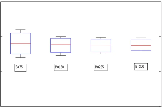
4.2.5.1 Criterion for Selecting the Number of Bootstrap Mod-els to be Constructed . . . 34
4.3 Case Study . . . 36
4.3.1 Case Study 1: The Four Branch Function . . . 36
4.3.1.1 Analysis . . . 36
4.3.1.2 Results . . . 37
4.3.2 Case Study 2: The Ishigami Function . . . 39
4.3.2.1 Analysis . . . 40
4.3.2.2 Results . . . 40
4.4 Chapter Summary . . . 41
5 Robust Surrogate Models - Random Model Parameters 43 5.1 Background Theory of Proposed Approach . . . 44
5.1.1 Bayesian Model Selection for Identical Trained Artificial Neural Networks . . . 44
5.1.2 Robust Artificial Neural Network Prediction . . . 46
5.1.3.1 Criterion for Selecting the Number of Identical
Net-works to be Constructed . . . 48
5.1.4 Adaptive Procedure for Robust Artificial Neural Network Train-ing . . . 48
5.2 Case Study . . . 51
5.2.1 Case Study 1: The 2-D Non-Linear Function . . . 51
5.2.2 Case Study 2: The Rosenbrock Function . . . 54
5.3 Chapter Summary . . . 56
6 Robust Surrogate Models - Model Structure and Random Model Parameters 58 6.1 Background to Problem . . . 58
6.2 Proposed Approach . . . 59
6.2.1 Formulation of Optimization Problem for Optimal ANN Archi-tecture and Training Sample Size Selection . . . 59
6.2.1.1 Searching Optimal ANN Solutions with Evolutionary Algorithm . . . 62
6.2.1.2 Encoding the Chromosome . . . 62
6.2.1.3 Procedures Taken to Search for Optimal Network Ar-chitectures . . . 63
6.2.1.4 Ensemble of Optimal Networks . . . 64
6.2.2 Bayesian Model Selection for Matrix Consisting of Identical ANNs 64 6.2.2.1 Robust Prediction from Artificial Neural Networks . 66 6.2.2.2 Confidence Interval for Robust Neural Network Pre-diction . . . 67
6.2.3 Model Averaging for the Ensemble of Robust Neural Networks 68 6.2.3.1 Combination of the Robust Networks Confidence In-tervals . . . 69
6.2.3.2 Criterion for Selecting the Number of Identical Net-works to be Constructed . . . 69
6.2.3.3 Adaptive Procedure for Optimized Robust ANN Train-ing . . . 69
6.3 Case Study . . . 72
6.3.1 Case Study 1 . . . 72
6.3.1.1 Analysis . . . 72
6.3.2 Case Study 2 . . . 76
6.3.2.1 Analysis . . . 77
6.3.2.2 Results . . . 77
6.4 Chapter Summary . . . 80
7 Uncertainty Quantification of the Site Ion eXchange Plant Using Robust Artificial Neural Networks 81 7.1 Overview . . . 81
7.1.1 Computational Model of the SIXEP . . . 82
7.1.1.1 Modelling the Uncertainty in the Model Input Param-eters . . . 85
7.2 Reliability Analysis of the SIXEP Using Robust Artificial Neural Net-works . . . 85
7.2.1 Analysis . . . 86
7.2.2 Results . . . 87
7.3 Sensitivity Analysis of the SIXEP Using the Proposed Approaches . . 88
7.3.1 Analysis . . . 89
7.3.2 Results . . . 89
7.4 Conclusion . . . 92
8 Fault Diagnosis of a Nuclear Power Plant Using Robust Artificial Neural Networks 93 8.1 Background to Problem . . . 93
8.1.1 Case Study: The Indian Pressurized Heavy Water Reactor (PHWR) 94 8.1.2 Aim and Objectives of Chapter . . . 95
8.1.3 Data Set for Training Predictive Model . . . 95
8.2 Fault Diagnostic by Robust ANN . . . 98
8.2.1 Case 1 . . . 98
8.2.2 Predicting Blind Case Data . . . 103
8.2.3 Case 2 . . . 104
8.2.3.1 Adapting the IIR-LRNN to the Multi-Objective Op-timization Framework . . . 104
8.2.4 Case 3 . . . 107
8.2.5 Proposed Framework for Combining Chapter 4 and 6 Approaches107 8.3 Chapter Summary . . . 110
9 Uncertainty Analysis of Spectral Correction Schemes in High-Energy Environments 111
9.1 Problem Definition . . . 111
9.1.1 Neutron Detectors for Measuring High-Energy Neutrons . . . 112
9.1.2 State-of-the-art . . . 112
9.1.3 Materials and Method . . . 113
9.1.3.1 Bonner Spheres and Neutron Dose Meters . . . 113
9.1.3.2 Neutron Spectra and Dose Correction Factors . . . . 115
9.1.4 Results and Discussion . . . 117
9.1.4.1 Characterising the Neutron Field . . . 117
9.1.4.2 General Trends in Spectral Correction Factors . . . . 118
9.1.4.3 Neutron Calibration Sources and Spectral Correction Factors . . . 121
9.1.4.4 Neutron dose meters and spectral correction factors . 122 9.1.5 Validation of the Proposed Models . . . 124
9.2 Uncertainty Analyses of the Spectral Correction Schemes . . . 127
9.2.1 Proposed Approach for Quantifying Uncertainty in Spectral Correction Schemes . . . 128
9.3 Chapter Summary . . . 136
10 Conclusions and Recommendations 138 10.1 Summary . . . 138
10.1.1 Research Contributions . . . 139
10.1.2 Applications . . . 140
List of Figures
1.1 Organisation of Chapters in Thesis . . . 7
3.1 Architecture of a 2 Hidden Layer Feed-forward Artificial Neural Net-work with Neurons . . . 20
4.1 Flow Chart for Adaptive Bootstrap Algorithm . . . 35
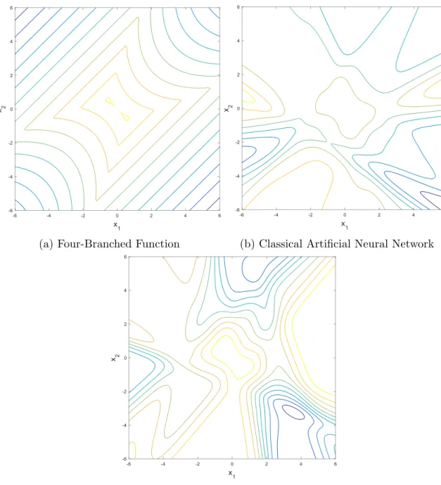
4.2 Limit State - Four branched Function . . . 36
4.3 Four-Branched Function - Visual Composition of Bootstrap Artificial Neural Network . . . 37
5.1 Flow Chart for Adaptive Robust ANN Algorithm . . . 50
5.2 Surface and Contour Plot of Limit State Function . . . 51
5.3 Limit State Surface Plot - Safety Function . . . 52
5.4 Surface and Contour Plot of Rosenbrock Function . . . 54
5.5 Surface and Contour Plot of Rosenbrock Function . . . 55
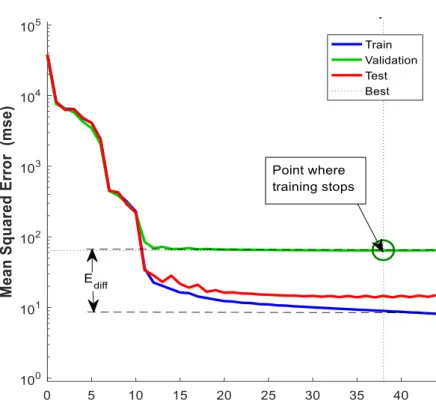
6.1 Region Where Edif f is Computed . . . 61
6.2 Flow Chart for Adaptive Optimized Robust ANN Algorithm . . . 71
6.3 Response Surface Plot - Safety Function . . . 74
6.4 Response Surface Plot - Resenbrock Function . . . 74
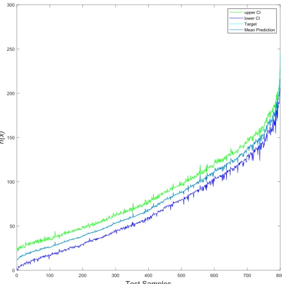
6.5 Robust ANN Prediction . . . 78
6.6 Kriging Prediction . . . 79
7.1 SIXEP Schematic [1] . . . 82
7.2 Black-Box Schematic of SIXEP . . . 83
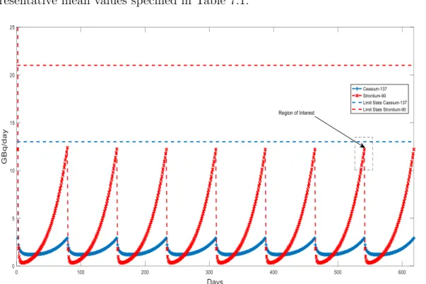
7.3 Deterministic Simulation from the SIXEP Model . . . 84
7.4 Bootstrap Confidence Intervals at Different Iterations of the Algorithm 87 7.5 Estimated Failure Probability Uncertainty Distribution for Different Number of Identical ANNs . . . 88
7.6 Confidence Intervals Caturing the Model Uncertainties for First Order Sensitivity Indices Estimate of 137Cs . . . 89
7.7 Confidence Intervals Caturing the Model Uncertainties for Total Effect
Sensitivity Indices Estimate of 137Cs . . . 90
7.8 Confidence Intervals Caturing the Model Uncertainties for First Order Sensitivity Indices Estimate of 90Sr . . . 90
7.9 Confidence Intervals Caturing the Model Uncertainties for Total Effect Sensitivity Indices Estimate of 90Sr . . . 91
8.1 PHT system of Indian PHWR . . . 94
8.2 Data Samples from South Inlet Header, PHT Pressure in South Hot Header, North Inlet Header, PHT Pressure in North Hot Header Re-spectively. . . 96
8.3 Illustration of Modelling Approach for Case 1 . . . 98
8.4 Performance of Robust ANN at Different Iterations of the Algorithm for Large Training Set. Top LeftM = 10, Top RightM = 20, Bottom Left M = 30, Bottom Right M = 40. . . 100
8.5 Performance of Robust ANN at Different Iterations of the Algorithm for Small Training Set. Top Left M = 10, Top RightM = 20, Bottom Left M = 30, Bottom Right M = 40. . . 102
8.6 Blind Case Data Set Prediction from Robust ANN. Top Figure, Break Level Prediction for 75% Break Size. Middle Figure, Break Level Pre-diction for 50% Break Size. Bottom Figure, Break Level PrePre-diction for 160% Break Size. . . 103
8.7 Illustration of Modelling Approach for Case 2 . . . 104
8.8 Blind Case Data Set Prediction from Robust RNN. Top Figure, Break Level Prediction for 75% Break Size. Middle Figure, Break Level Pre-diction for 50% Break Size. Bottom Figure, Break Level PrePre-diction for 160% Break Size. . . 106
8.9 Illustration of Modelling Approach for Case 3 . . . 107
8.10 Blind Case Data Set Prediction from Robust IIR-LRNN. Top Figure, Break Level Prediction for 75% Break Size. Middle Figure, Break Level Prediction for 50% Break Size. Bottom Figure, Break Level Prediction for 160% Break Size. . . 110
9.1 Methodology Followed in [2] . . . 113
9.2 Bonner Sphere Spectrometer - Neutron Detector . . . 114
9.4 Approximation of the spectrum-dependent dose correction factors for the 9-inch Bonner sphere (calibrated with 252Cf) using the flux percent-age of high-energy neutrons in the spectrum and a comparison with our previous result. . . 120 9.5 Spectrum-dependent dose correction factors for the 4P68Bonner sphere
(calibrated with 252Cf) as a function of the flux percentage of high-energy neutrons in the spectrum. . . 120 9.6 Approximation of the spectrum-dependent dose correction factors for
the 9-inch Bonner sphere (calibrated with 252Cf) using the ratio be-tween the responses of two Bonner spheres (4P68 versus 6-inch) and a comparison with the result in [2] . . . 121 9.7 Comparison of the spectrum-dependent dose correction factors for the
9-inch Bonner sphere calibrated with 252Cf, 241Am – Be and 239Pu – Be neutron sources. . . 122 9.8 Comparison of the spectrum-dependent dose correction factors for four
Bonner spheres (6-inch, 7-inch, 8-inch and 9-inch) calibrated with a 252Cf neutron source. . . . 123 9.9 Flow Chart for Adaptive Bootstrap Algorithm . . . 125 9.10 Validation of the proposed curve fitting in Figure 9.4 by considering
1000 randomly generated neutron spectra representing various work-places. . . 126 9.11 Validation of the proposed curve fitting in Figure 9.6 by considering
1000 randomly generated neutron spectra representing various work-places. . . 127 9.12 Flow Chart of Algorithm for Quantifying the Uncertainty in the
Spec-tral Correction Schemes . . . 130 9.13 Spectral Correction Schemes (Quadratic Model) with 95% Confidence
Intervals at Differetnt Iteration Levels . . . 132 9.14 Spectral Correction Schemes (Linear Model) with 95% Confidence
In-tervals at Differetnt Iteration Levels . . . 133 9.15 Spectral Correction Schemes (Linear Model) with 95% Confidence
In-tervals at Differetnt Iteration Levels . . . 134 9.16 Spectral Correction Schemes (Quadratic Model) with 95% Confidence
Intervals at Differetnt Iteration Levels . . . 135 9.17 Model Average of the Prediction from the Linear and Quadratic Model 136
List of Tables
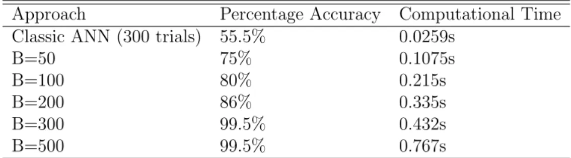
4.1 Accuracy of Method for Four-Branched Function . . . 38
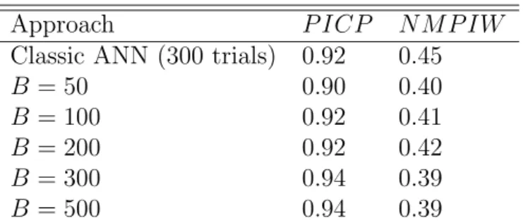
4.2 Prediction Intervals Performance Comparison Between the Proposed Approach and Classical Approach . . . 39
4.3 First Order Sobol’ Indices . . . 40
4.4 Total Effect Indices . . . 40
4.5 Accuracy of Method for Ishigami Function . . . 41
4.6 Prediction Intervals Performance Comparison Between the Proposed Approach and Classical Approach . . . 41
5.1 Estimate of the Failure Probability Using Robust ANN . . . 52
5.2 Accuracy of Proposed Approach - 2-D Non-Linear Function . . . 53
5.3 Prediction Intervals Performance Comparison Between the Proposed Approach and Classical Approach . . . 53
5.4 Estimate of the Failure Probability Using Robust ANN . . . 55
5.5 Accuracy of Proposed Approach - Rosenbrock Function . . . 56
5.6 Prediction Intervals Performance Comparison Between the Proposed Approach and Classical Approach . . . 56
6.1 Optimal ANN Architectures from GA Optimization - Safety Function 72 6.2 Optimal ANN Architectures from GA Optimization - Resenbrock Func-tion . . . 72
6.3 Estimate of the Failure Probability Using Robust ANN . . . 73
6.4 Estimate of the Failure Probability Using Robust ANN . . . 73
6.5 Accuracy of Method for 2D-Non-Linear Function . . . 75
6.6 Prediction Intervals Performance Comparison Between the Proposed Approach and Classical Approach . . . 75
6.7 Accuracy of Method for Rosenbrock Function . . . 75
6.8 Prediction Intervals Performance Comparison Between the Proposed Approach and Classical Approach . . . 76
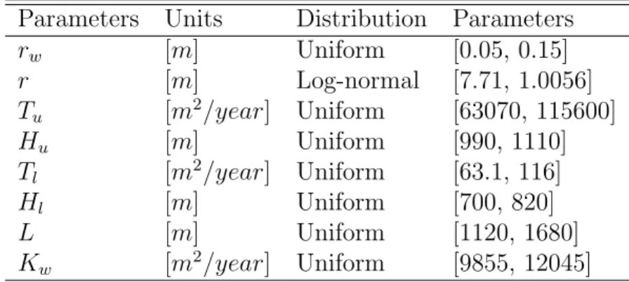
6.9 Borehole Model Definition of the Probabilistic Model of the Input
Pa-rameters . . . 77
6.10 Prediction Intervals Performance Comparison Between the Proposed Approach and Classical Approach . . . 79
7.1 Random Variables used to Represent the Uncertainties of the SIXEP Feed Inputs . . . 86
7.2 Percentage Accuracy of Chapter 4 Approach . . . 91
7.3 Percentage Accuracy of Chapter 5 Approach . . . 91
8.1 List of selected process parameters for LOCA identification . . . 97
8.2 Artificial Neural Network Architectures Discovered by Genetic Algo-rithm for Large Data Set. . . 99
8.3 Artificial Neural Network Architectures Discovered by Genetic Algo-rithm for Small Data Set. . . 101
Chapter 1
Introduction
”Personally, I see research like riding a bicycle, the more I push the pedal, the more I discover new ideas.”
1.1
Context
In state-of-the-art engineering practices, mathematical models are used to represent physical processes or engineering processes systems. There are vast applications of these models in various disiplnes such as the modelling of nuclear waste management systems (see [1]), the modelling of buildings with finite element models (FEM) (see [3]) etc. The mathematical model aims at replicating the behaviour of the physical system for a given set of input parameters. For example, the nuclear waste manage-ment model may predict the concentration levels of a particular radionuclide for a given period of time. The set of the model input parameters may include the physical and mechanical properties of the radioactive waste plant. On the other hand, due to the diversity of the applications and the kind of the analyses to be performed, the complexity of the mathematical model may range from simple analytical functions to complex mathematical equations (e.g. partial differential equations). Often, complex mathematical equations have no unique solution method, but rely on solvers such as finite element or finite difference schemes. Nowadays, a large number of commercial and non commercial software packages have been developed intending to solve these complex mathematical models. Despite the advances in these software packages, they all tend to be simplifications of reality. When having identified a suitable mathemat-ical model, different sources of inaccuracies may occur. As the mathematmathemat-ical model represents a simplification of reality, it usually contain model error. Additionally, these numerical models introduce numerical discretization errors. Most importantly,
the parameters of a mathematical model might not be known precisely. The differ-ent types of uncertainties might or might not be presdiffer-ent in a given problem setting. Hence, it is important to quantify the uncertainties in order to be able to interpret the results realistically. The main source of uncertainty identified in this literature is Aleatory uncertainty. Aleatory uncertainty (from Latin alea, rolling of dice), also called variability, refers to the intrinsic randomness of a natural phenomenon, which cannot be reduced by acquiring more data, and is described using probabilistic mod-els. In the multidisciplinary design of complex critical systems, ignoring the effect of uncertainty is unacceptable, as it may lead to catastrophic consequences. Addi-tionally, complex critical systems involve high-consequence decisions often made on the basis of quantitative data that is very scarce or prohibitively expensive to collect. Despite the availability of detailed high fidelity physical models, engineering practi-tioners still need to make clear decisions based on available information. Thus, they must be able to trust the methodology adopted to analyse the system, in order to quantify the risk with the available level of information, and so avoid wrong deci-sions due to artificial restrictions introduced at the modelling stage. Comprehensive modelling of uncertainty that accounts for inherent variability provide insight into engineering problems, enabling robust decisions to be made. Risk is conventionally understood as the product between the failure probability of the system and the ex-pected loss (or consequence) caused by the system failure. While the exex-pected loss is quantified in monetary units, the failure probability is calculated, by means of re-liability methods, within a rigorous mathematical framework. Usually, this requires the specification of precise distribution models (of probability), including dependen-cies for the input variables. The uncertainty management requires the uncertainty to be propagated, quantified and the risk to be assessed and subsequently minimised. Likewise, a system performance can only be improved if the parameters that affect the performance significantly are identified and focused on. Sensitivity analysis is used to achieve this by identifying and ranking the contributions of parameters of the system to the variability in the output quantity of interest. Most often, the variance based method to sensitivity analysis [4] is adopted when assessing the contributions of the state variables. This method is a class of simulation approaches that is used to decomposes the output variance into parts that can be attributed to the inputs and interactions between them. Usually, engineering models are often quite detailed and may require several hours for a single deterministic analysis. On the other hand, to quantify the effect of uncertainty on these systems, models need to be evaluated several times with different combinations of the input parameters. Obviously, this
leads to a computational problem, as a repeated number of model calls is required for robust analyses. Therefore, the development of fast accurate surrogate models is key to make the uncertainty quantification ever closer to the community of engineering practitioners.
1.2
General Framework for Uncertainty
Quantifi-cation in this Thesis
Uncertainty Quantification (UQ) is a general term to summarize the various task and challenges described previously. A summary of the main elements of UQ framework is listed in the following steps:
Step 1: The computational model representing the physical system or process may con-sist of an analytical function in the simplest case. However, the computational model may also consist of an entire work-flow containing different pieces of software coupled together or even physical experiments. In general, the compu-tational model map a set of input parameters to the quantity of interest that is used in decision making.
Step 2: The characterisation of input parameter uncertainties aims at identifying the type of uncertainty and modelling them adequately. A variety of modelling choices for different types of uncertainties are available, which includes con-stants (i.e. no uncertainty), probability distributions, intervals, and imprecise probabilities. The suitability of an uncertainty model depend on various fac-tors such as the availability of information of the input parameters, general knowledge of the system being analysed, as well as the purpose of the analysis. For the purpose of this thesis, probability distributions which comes under the framework of probability theory will be used to model the parameter uncertain-ties.
Step 3: Uncertainty propagation analyses how the uncertainty in the input parameters is transformed through the computational model towards the quantity of in-terest in the output of the model. When the input is modelled by uncertain parameters, the quantity of interest is likely to be uncertain too. Hence, this step analyses different statistics of interest, depending on the problem at hand. In this thesis, the statistics of interest include the failure probabilities, and sensitivity indices.
1.3
Problem Statement
In the general framework for UQ, there are various challenges. Starting from Step 1, consider the computational model that represents the physical system being anal-ysed (i.e. FEM model representing a building). The model may be complex (i.e. large number of parameters) and expensive to evaluate such that a single run of the computational model takes minutes, hours or even days to converge to a solu-tion. The computational model is usually given as a black box such that only the input parameters and the output quantity of interest are observable. Thereafter, in Step 2, probability theory is used to characterize and model the aleatory uncertainty. Nevertheless, when the computational model at hand is expensive to evaluate due to complexity of the model, the total computational cost is dominated by increased wall-clock time. Consequently, surrogate-modelling (also called response surface and meta models) techniques are widely established in probabilistic settings. Surrogate mod-els approximate the expensive computational model by a simple and inexpensive to evaluate function. Subsequently, these surrogate models can be used for uncertainty propagation analyses such as reliability analysis and sensitivity analysis, allowing for high number of model evaluations for reduced wall-clock time. Contrarily, the use of a surrogate model for this kind of analysis can introduce some additional uncertainty into the quantity of interest sorted out. Clearly, there is a need to quantify the addi-tional uncertainties introduced by the surrogate model in order to ensure robust and reliable results, in particular, when the results obtained from the surrogate model is used for decision making.
1.4
Objectives of the Thesis
Considering the problem statement, this thesis is focused on the following objectives: • To develop intuitive frameworks to quantify the surrogate model uncertainties. • To utilize state-of-art surrogate modelling techniques to conduct uncertainty
quantification analysis in the presence of aleatory uncertainties.
• To apply the proposed frameworks to a variety of classical uncertainty quantifi-cation analyses problems, such as structural reliability analysis and sensitivity analysis.
• To show the relevance of the proposed frameworks for other realistic nuclear engineering problems.
1.5
Original Contributions
This thesis provides numerical techniques that contributes to the field of surrogate modelling for Uncertainty Quantification and Regression Analysis. Although the techniques proposed in this thesis was originally meant for artificial neural networks, it can easily be adopted to different classes of surrogate models. Particularly, the techniques developed in this thesis are used for quantifying the model uncertainties introduced when using a surrogate model for Regression Analysis, and Uncertainty Quantification. the sources of uncertainties considered in this thesis originates from:
• Variability in training data set. • Random model parameters. • Structure of the model
To the author knowledge, there is no generalized numerical framework that tackles all theses sources of uncertainties affecting the performance of a surrogate model used in the aforementioned tasks. Thus, there is a need to develop such techniques, particularly, when surrogate models are used for safety critical applications.
1.6
Numerical Implementation
The quantification of surrogate model uncertainty require the availability of flexible numerical tools. For these reasons, the proposed numerical frameworks have been developed and integrated into OpenCossan (see [5]). OpenCossan is a collection of open source algorithms, methods and tools released under the LGPL licence, and under continuous development at the Institute for Risk and Uncertainty, University of Liverpool, UK. The source code of the software is available upon request. OpenCos-sanis also the computational core of the general purpose software, called COSSAN-X, which was originally developed by the research group of Prof. G.I. Schuller at the University of Innsbruck, Austria [6]. The term general purpose software implies that a wide range of engineering and scientific problems can be treated with a single software. The computational core of the software is developed in MATLAB object-oriented environment, which includes several predefined solution sequences to solve problems from different fields. The framework is organized in classes, consisting of properties and methods together with their interactions and interfaces. Thanks to the modular nature of OpenCossan, it is possible to define specialized solution se-quences for robust surrogate modelling and parallel computing strategies to reduce
the overall cost of implementing the proposed framework to the practical engineering problems in this thesis.
1.7
Outline of Thesis
The organisation of chapters in this thesis follows the simple structure shown in Figure 1.1. In Chapter 2, the theoretical background of uncertainty modelling, propagation and quantification is introduced. Thereafter, Chapter 3 gives a brief overview of the state-of-the-art in surrogate modelling, with emphasis paid to Artificial Neural Net-works (ANNs). In Chapter 4, an adaptive bootstrap technique used to quantify the model uncertainties of ANN originating from variability in training data. In Chapter 5, a framework used to deal with model uncertainties originating from random pa-rameters of the surrogate model is introduced. Subsequently, Chapter 6 extends the framework introduced in Chapter 5 by including another framework that considers the model uncertainties originating from the structure of the surrogate model. The applicability of the proposed frameworks in Chapter 4 and 5 are tested on real case study in Chapter 7. Furthermore, in Chapter 8, the framework developed in Chap-ter 6 is tested on another real case study concerning fault diagnostic of a nuclear power plant. In addition, the approach developed in Chapter 4 is combined with the approach in Chapter 6 and applied to the same case study. In Chapter 9, the framework proposed in chapter 4 is applied to real Nuclear engineering problem faced at high-energy neutron facilities. Lastly, some conclusions and recommendations are provided in Chapter 10, summarising the presented work and indicating directions for potential future developments.
Numerical Development Chapter 4 Chapter 5 Chapter 6 Applications Chapter 7 Chapter 8 Chapter 9 Theoretical Background Chapter 2 Chapter 3
Chapter 2
Modelling and Quantification of
Parameter Uncertainties
Parameter uncertainty can be modelled by a variety of concepts. In this chapter, random variable which is the selected choice to model aleatory uncertainty in this thesis is discussed. In addition, uncertainty propagation and quantification techniques such as reliability and sensitivity analyses are discussed.
2.1
Modelling Aleatory Uncertainty
2.1.1
Probability Theory
In a probability space (Ω,F,P), Ω denotes an event space (also called sample space, universal set, or outcome space) equipped with the σ-algebra F and a probability measure P ∈ [0,1]. Furthermore, for an event E ∈ Ω, and its complementary event Ec, by definition, their union is given asE ∪ Ec = Ω and their intersection gives a zero
eventE ∩Ec= Ø. Hence, the probability ofE andEcadd up to one:
P(E)+P(Ec) = 1.
The respective probability of the empty set Ø and the complete set are given as
P(Ø) = 0 and P(Ω) = 1. With this condition, a random variable X is defined by
the mapping X(ω) : Ω 7→ DX ⊂ R, where ω ∈ Ω is an elementary event and DX is
the support domain of X. A realization of the random variable X is denoted by the corresponding lower case letter x. A random variable X is normally characterized by a cumulative distribution function (CDF) FX which assigns a probability to the
event {X ≤ x}, i.e. FX(x) = P(X ≤ x). From this definition, any CDF that is
monotonically non-decreasing, tends to zero for low values ofx, and tends to one for large values of x. For continuous random variables, the first derivative of the CDF is the probability density function (PDF) and is denoted by fX(x) = dFX(x)/dx.
The PDF describes the likelihood ofX being in the neighbourhood ofx. Due to the monotonicity property of CDFs, fX(x)≥0 for all x∈ DX.
2.1.1.1 Data to Cumulative Distribution Function Empirical Cumulative Distribution Function
Consider a set of sample realizations χ = {χ(1), ..., χ(N)} of a random variable X, whose probability distribution is not known. To describe χ properly, the data χ is used to deduce a probability distribution. A basic method of statistics is then to compute the empirical CDF, which is defined as:
FXemp= 1 N N X i=1 Ix≥χ(i)(x), (2.1)
where I is the indicator function, which indicates I = 1 for a true subscript state-ment and I = 0 otherwise. As the number of samples N are limited, the empirical CDF is a stair-shaped curve with constant CDF values between samples and steps at x =χ(i), i = 1, ..., N. Assuming that the probability distribution X may be con-tinuous, the empirical CDF provides a poor but simple estimate of FX. Thus, more
sophisticated methods, such as the method of moments or the maximum likelihood method, are usually adopted for practical purpose.
Method of Moments
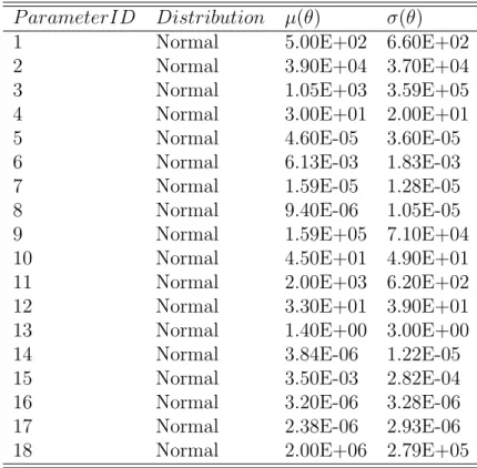
Here, a distribution family FX(x|θ) is considered, where θ denotes a vector of pa-rameters that defines the shape of the CDF. In addition, the number of papa-rameters is denoted as nθ = |θ|. Commonly used distributions in literature and practice,
have nθ = 2. Next, the method of moments determines the optimal distribution by
matching the first moments ofFX(x|θ) with the sample-based estimations of the first
moments based on χ, by denoting the mean value and variance of X by µ(θ) and
σ2(θ), which depend on the yet-to-be-determined parameters θ. Further, the sample mean and variance is given byE[χ] and V ar[χ]:
E[χ] = 1 N N X i=1 χ(i), (2.2) and, V ar[χ] = 1 N −1 N X i=1 (χ(i)−E[χ])2. (2.3)
The parametersθare obtained by solving: µ(θ) =E[χ],σ2(θ) = V ar[χ]. The method of moments relies on the knowledge of the underlying distribution family, which is
an additional assumption compared to the empirical CDF. However, this assumption avoids the stair-shaped CDF curves of the empirical CDF, thus providing a smooth CDF curve.
Maximum Likelihood Method
Analogous to the method of moments, the maximum likelihood method requires the knowledge of a distribution family FX(x|θ) with unknown distribution parameters θ. Thereafter, the likelihood of observing χ depending on the parameter value θ is computed by: L(θ|χ) = N Y i=1 fX(χ(i)|θ), (2.4)
wherefX(x|θ) is the PDF conditional onθ. The optimal parameter values are deduced by maximizing the likelihood function:
θ∗ =arg max
θ L(θ|χ). (2.5)
The practicability of the method depends on the initial assumption on the distribu-tion family. In fact, any distribudistribu-tion family can be fitted using this method.
2.2
Quantification of Parameter Uncertainties
Once the parameter uncertainty has been modelled with a PDF, propagation of the parameter uncertainties through the model to the quantify of interest is required for an adequate quantification of the uncertainties. To quantify the performance of complex critical systems in the presence of the parameters uncertainties, reliability analysis is carried out. Similarly, a system performance can only be improved if the parameters that affect the performance significantly are identified and focused on. Sensitivity analysis is used to achieve this by identifying and ranking the contributions of each state variable of the system to the variability in the performance. Henceforth, the following sections provides a concise discussion on the theory of reliability and sensitivity analysis using the simulation approach.
2.2.1
Reliability Analysis of Systems
Reliability methods is a powerful technique used in various engineering disciplines to quantify the performance of the system under investigation in the presence of param-eter uncertainties. The aim of reliability methods is producing a design that meets
some predefined performance objectives. For example, during the lifetime of a struc-ture, a series of conditions that depends on external actions affects the performance of the structure. Usually, the external actions are random processes in space and time. Hence, the external actions affect the structural responses. The structural re-sponses are referred to as demands, while the thresholds that the rere-sponses are not allowed to exceed are referred to as capacities. Further, the space of all demands and capacities is referred to as state space which is used to form the limit state surface of the structure. The intersection and union of this limit state surfaces define two mutually exclusive domains: the failure domain, χF , and the survival domain, χS.
A random state,x, of the system, which includes the demands and capacities, can be represented as a point in the state space, where the structure is in a ”safe” state if the point is strictly contained in the safe domain,x ∈χS, whereas it is in a ”failed”
state if contained in the failure domain, x∈χF . The reliability, pR, is formulated as the probability of a random state to be in the safe domain, whereas, the probability of failure,pF is the probability of a random state to be in the failure domain. Hence, pF +pR = 1. In the state space, some reliability metrics can be defined to assess
to what extent the structure can be considered safe. For instance, it is common to refer to the distance between a random state and the limit state surface as the safety margin. The failure probability pF is defined as:
pF = Z · · · Z χF fX(x1, . . . , xd)dx1. . . dxd, (2.6)
where, fX denotes the joint density function, and d is the number of model input
parameters. In general, the integral of Eq. (2.6) is difficult to calculate analyti-cally, due to the multi-dimensional nature of the integral. Thus, its estimation can be analytically intractable, especially for complex systems with a large number of parameters.
2.2.1.1 Estimation of the Failure Probability by means of Simulation
Consequently, various methods have been proposed to computepF in recent and past literature. The first attempts were oriented towards using analytical methods [7]. Afterwards, numerical methods based on the calculation of the performance function Hessian [8] or asymptotic approximation [9] were increasingly used. Conversely, these numerical methods becomes inefficient as the number of parameters increases, thus, the error in the estimate of pF increases for complex models. Hence, simulation
MC simulation is independent of the system complexity and is the most flexible method to estimate pF [6]. Fundamentally, MC simulation is performed by means
of sampling a large number of realisations from the joint distribution, x, from given probability distributions, thereafter counting the number of “safe” samples over the total number of samples. Specifically, an indicator function, IF , is used to label the
states, such that it indicates zero if “safe” and one if “unsafe”. Thus, the failure probability is estimated as:
pF = ∞ Z −∞ ∞ Z −∞ IF[x∈χF]fX(x1, ..., xd)dx1, ..., dxd. (2.7)
If the samples generated, x{s}, s = 1, ..., N
s, follows the pattern of the distribution fX, Eq. (2.7) can be approximated by:
ˆ pF = 1 Ns Ns X s=1 IF[x{s}]∈χF, (2.8)
by generating a large number of samples,Ns, which provides an unbiased estimation of the failure probability. The accuracy of the estimate of Eq. (2.8) solely depends on the number of samples generated and can be assessed computing the coefficient of variation, CoV , of the estimator, ˆpF. The CoV of the failure probability estimator
is defined as: CoV[ˆpF] = r 1−pF pF ×Ns . (2.9)
This simply means that a sample size Ns > 1/pF is required for CoV[ˆpF] < 1 and
acceptable values, where CoV[ˆpF] < 0.3, can be obtained for Ns = 10/pF. Thus, a
large number of model evaluations are required by the method in order to assess the indicator function, IF. The large number of model evaluations can be infeasible in realistic engineering practices, as the computational time for a single model evaluation can be long. Subsequently, the limitations of direct Monte Carlo can be mitigated by resorting to Advanced Sampling methods, such as Importance Sampling (IS) [12], Line Sampling (LS) [3, 13], Subset Simulation (SS) [14, 15], etc. Importantly, each of these simulation method carries their own special performance feature to target different classes of problems. For instance, LS is specially suited to estimate small failure probabilities in high dimensional spaces, provided that the limit state surface displays a single failure mode. However, the use of advanced sampling technique comes with several limitations that could affect the accuracy of the targeted failure probabilitypF.
should know what region of the space to sample from, as IS may underestimate the target failure probability if the proposal distribution does not cover the whole failure region. Similarly, the LS technique requires setting up an important direction which is defined as the direction pointing towards the region of interest. However, a priori knowledge about the system failure domain is required before defining the important direction. Contrarily, LS has been found to significantly outperform SS, in particular in the task of estimating very small failure probabilities (i.e., around 10−7) (see [16]).
2.2.2
Sensitivity Analysis of Systems
On the other hand, a system performance can only be improved if the state variables that affect the performance significantly are identified and focused on. Sensitivity Analysis (SA) is used to achieve this by identifying and ranking the contributions of the input parameters to the variability in the output quantity of interest. Different classes of SA methods can be found in the literature [17–19]. Specifically, the methods are divided into two classes, namely local and global SA methods. In local SA, the effect of small variations in the input variables to the quantity of interest are investigated, whereas global SA focuses on the entire variation of the input variables. In this thesis, global SA methods are focused on. Commonly, global SA methods are developed under the framework of the probability theory, i.e. the uncertainty in the input variables is modelled as random variables. Thus, a large number of evaluations of the computational model for different realizations of the input random variable is required. In this thesis, the variance-based sensitivity analysis method often referred to as Sobol’ indices is adopted. In the context of probability theory, the variance based method decomposes the variance of the output quantity of interest into fractions which can be attributed to the inputs. From a black box perspective, the model under investigation is viewed as a function y =f(x), where x is a vector of d uncertain model inputs x1, x2, ..., xd, and y is a chosen univariate model output
(note that this approach examines scalar model outputs, however multiple outputs can be analysed by multiple independent sensitivity analyses). Furthermore, it is assumed that the inputs are independently and uniformly distributed within the unit hypercube, i.e. xi ∈[0,1] for i= 1,2, ..., d. This incurs no loss of generality because any input space can be transformed onto this unit hypercube. Thus, f(x) may be decomposed as: y=f0+ d X i=1 fi(xi) + d X i<j fij(xi,xj) +· · ·+f1,2,...,d(x1,x2, ...,xd), (2.10)
where f0 is a constant and fi is a function of xi, fij a function of xi and xj, etc. A
condition of this decomposition is that: Z 1
0
f1,2,...,d(x1,x2, ...,xd)dxd = 0, (2.11)
i.e. all the terms in the functional decomposition are orthogonal. This leads to defi-nitions of the terms of the functional decomposition in terms of conditional expected values:
f0 =E(y), (2.12)
fi(xi) = E(y|xi)−f0, (2.13)
fij(xi,xj) =E(y|xi,xj)−f0−fi−fj. (2.14)
It can be seen that fi is the effect of varying xi alone which is the main effect of xi,
and fij is the effect of varying xi and xj simultaneously, additional to the effect of
their individual variations. This is known as a second-order interaction. Higher-order terms have analogous definitions. Further assuming that thef(x) is square-integrable, the functional decomposition may be squared and integrated to give:
Z 1 0 f2(x)dx−f02 = d X i=1 d X 1<...<d Z f12,2,...,ddxi, ..., dxd. (2.15)
Notice that the left hand side is equal to the variance ofy, and the terms of the right hand side are variance terms, now decomposed with respect to sets of the xi. This
finally leads to the decomposition of variance expression:
V ar(y) = d X i=1 Vi+ d X i<j Vij +· · ·+V1,2,···,d, (2.16) where, Vi =V arxi(Ex i(y|xi)), (2.17) and Vij =V arxij(Ex ij(y|xij)). (2.18)
A direct variance-based measure of sensitivity Si, called the first-order sensitivity index, or main effect index is stated as follows:
Si = Vi
V ar(y). (2.19)
This is the contribution to the output variance of the main effect of xi, therefore it
parameters. It is standardised by the total variance to provide a fractional contri-bution. Higher-order interaction indices such asSij can be formed by dividing other
terms in the variance decomposition by V ar(y). Note that this has the implication that, d X i=1 Si+ d X i<j Sij +· · ·+S1,2,...,d = 1. (2.20)
Using the Si, Sij and higher-order indices given above, one can visualize the signifi-cance of each variable in the output variance. However, when the number of variables is large, this requires the evaluation of 2d−1 indices, which can be too computa-tionally demanding. For this reason, a measure known as the Total-effect index, Ti,
is used. This measures the contribution to the output variance of xi, including all
variance caused by its interactions, of any order, with any other input variables. It is given as:
Ti = 1−
V arx i[Ex i(y|x i)]
V ar(y) . (2.21)
2.2.2.1 Estimating Sobol’ Indices by means of Monte Carlo Simulation
Subsequently, to estimate Sobol’ indices, MC sampling based methods have been developed in several literatures. For example, in ref [20], a method for estimating the Sobol’ first order and interaction indices have been developed. Additionally, in ref [17] a method for estimating the first order and total indices have been developed. Unfortunately, to get robust estimates of sensitivity indices, both methods are costly in terms of the large number of model runs required. Consequently, using quasi-Monte Carlo sequences such as Sobol sequence [21] or Latin hypercube sampling (LHS) [22] for sample generation instead of the classic Monte Carlo (MC) method can sometimes reduce the number of model runs by a factor ten [23]. Furthermore, in the Fourier Amplitude Sensitivity Test (FAST) method [24], a single frequency variable is used to represent a multivariate function in the frequency domain. Thus, the integrals required to compute the Sobol’ indices become univariate, resulting in low number of model calls. Consequently, ref [25] have extended the FAST method to compute total Sobol’ indices. In addition, ref [26] have coupled FAST method with a Random Balance Design. Recently, ref [27] have analysed and improved these methods. Contrarily, FAST remains expensive, unstable and biased when the number of inputs increases [27]. On the other hand, the advantages of using a MC based method to compute the sensitivity indices is that it provides error made on indices estimates via random repetition or bootstrap methods. Thus, MC based methods are
widely used. Generally speaking, using MC technique to estimate Si and theTi, the
total number of model calls follows the relationshipN(d+2). Hence, such analyses can become intractable when the computational model is expensive-to-evaluate. Then, the use of surrogate models is a popular solution to lower the total computational costs. The following chapter gives a brief overview of surrogate models.
2.3
Chapter Summary
The concepts presented in this chapter gives an overview of how the uncertainty in the model input parameter can be modelled, propagated and quantified within the context of the probabilistic theory. Subsequently, in an attempt to reduce the number of model calls for quantifying the parameter uncertainties, different techniques have been proposed. However, even for the most efficient technique proposed, the number of model calls are still large. Therefore, easy-to-evaluate surrogate models that can be used to replace the expensive models are required to reduce the computational cost. The following chapter gives the current state-of-the-art surrogate modelling techniques available.
Chapter 3
Classical Surrogate Models
This chapter gives an overview of the current state-of-the-art surrogate modelling techniques used for Uncertainty Quantification. In particular, feed-forward Artificial Neural Network and Deep Neural Networks are focused on.
3.1
State of the Art
Uncertainty Quantification (UQ) usually requires a large number of model calls for different input values through a MC simulation procedure. Such approach requires thousands to millions of model calls which is not affordable in many practical cases even with high-performance computing. Subsequently, a viable approach to reduce the computational burden associated to UQ is resorting to easy-to-evaluate surrogate models, also called response surfaces or meta-models. These surrogate models are used in place of the high fidelity expensive model. Although they are fast, they still require the same number of model calls required for UQ, but require a lesser wall-clock time. Furthermore, the construction of surrogate models require running the expensive moddel a predetermined number of times (e.g., 50-100 or more) via design of experiment techniques (see [28]) for specified range of the input variable space. Then, collecting the corresponding values of the output of interest. Thereafter, sta-tistical techniques are used to calibrate the internal parameters of the surrogate model in order to capture the underlying behaviour of the expensive model. The popular types of surrogate models include polynomial chaos expansions (PCE) [29], Kriging (also known as Gaussian process) [30–32], support vector machines (SVM) [33], ra-dial basis function (RBF) [34], reponse surfaces [35], and artificial neural networks (ANNs) [36], which have been extensively investigated in the last decade. Recent development in surrogate modelling such as PC-Krigin have been proposed in ref [37]. This current development combines classical PCE and Kriging. Furthermore,
it has been shown to perform better than either PCE or Kriging (see [37]). Several literatures can be found concerning the application of these aforementioned surrogate models in UQ analysis. For example, in refs [38–40], response surfaces are employed to evaluate the failure probability of structural systems. In [41–44], surrogate models such as ANNs, RBF and SVM are trained to provide local approximations of the failure domain in structural reliability problems. In [45, 46], Kriging models are used to speed up the computation of the global sensitivity indices for a complex hydro-geological model simulating radionuclide transport in groundwater. Finally, in the literature [37, 47, 48] a vast number of surrogate modelling techniques are used for UQ problems. Furthermore, comparing the accuracy of the aforementioned surrogate modelling techniques, Kriging models tend to gives the best predictive performance due to the capabilities of their correction of the trend function, which ensures that the model passes for the value of every sample. Particularly, on small datasets (i.e. small number of samples and low model complexity), Kriging models are accurate because of this well-tuned smoothing property and cheap computational cost. However, for a large multi-dimensional data set (i.e. large number of training samples and complex model) Kriging models tends to under-perform. Thus, a surrogate model that can scale to large datasets and can generalize globally is needed. For this reason, ANNs are been chosen as the primary surrogate models in this thesis. The following sections gives a brief background to ANNs.
3.2
Background to Neural Networks
The human brain is complex machine able to solve complex problems. Although humans have a basic understanding of some of the operations that drive the brain, we are still far from understanding everything there is to know about the brain. Subsequently, in order to understand ANNs, a basic knowledge is required on how the brain functions. The brain is part of the central nervous system and consists of a very large neural network. The neural network in the brain is complicated, but will be simplified for the basic knowledge needed to understand ANNs. The neural network is a network that consist of connected neurons. The center of the neuron is called the nucleus. The nucleus is connected to other nucleus by means of the dendrites and the axon. This connection is called a synaptic connection. The neuron can send electric pulses through its synaptic connections, which is received at the dendrites of other neurons. In particular, when a neuron receives enough electric pulses through its dendrites, it activates and fires a pulse through its axon, which
is then received by other neurons. As a consequence, information can propagate through the neural network. Note that the synaptic connections change throughout the lifetime of a neuron and the amount of incoming pulses needed to activate a neuron also change. As a result, this continuous change allows the neural network to learn efficiently. Generally speaking, the human brain consists of around 1011 neurons which are highly interconnected with around 1015 connections [49]. These neurons activate in parallel as an effect to internal and external sources. The brain is connected to the rest of the nervous system, which allows it to receive information by means of the five senses and also allows it to control the muscles.
3.2.1
Artificial Neural Network
Currently, it is not possible to make an artificial brain, however it is possible to make simplified artificial neurons and ANN. Importantly, an ANN is not intelligent, but is good for recognizing patterns and approximating non-linear functions. ANN approx-imate non-linear functions on the basis of learning-by-example, meaning that when it is presented with training examples of the underlying function, it can generalize from these examples in order to approximate the actual function. The task of the ANN is to approximate the output of a function for any valid input, after having seen input-output examples for only a small part of the input space. ANN also have excellent training capabilities which is why they are often used in artificial intelligence research.
3.2.1.1 The Artificial Neuron
The idea of the artificial neuron was proposed by [50], but until [51] proposed the back-propagation algorithm that more focus was paid to ANN research. Currently, the most widely used kind of ANN is the multi-layered feed-forward ANN (FF-ANN), which consists of multiple layers of artificial neurons. The neurons are connected by connections which only go forward in between the layers. The back-propagation algorithm and most other related algorithms trains an ANN by propagating an error value from the output layer and back to the input layer while altering the connections on the way. A multilayer FF-ANN consists of neurons and connections. The neurons are located in layers and the connections go forward between the layers. Each neuron receives multiple inputs from others via connections that have associated weights, analogous to the strength of the synapse. When the weighted sum of inputs exceed the threshold value of the node, it activates and passes the signal through an activation
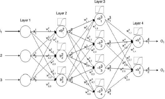
function and sends it to neighbouring nodes. Figure 3.1 shows a network architecture of a 2 hidden layer feed-forward network.
Figure 3.1: Architecture of a 2 Hidden Layer Feed-forward Artificial Neural Network with Neurons
More formally, if we call ai
j the activation value of the jth neuron in theith layer,
where a1
j is the jth element element in the input vector. Then, the next layer input
can the related to the previous layer input via the following relationship:
aij =κ(X
k
(wjki ×aki−1) +bij), (3.1)
whereκis the activation function,wi
jk is the weight from thekthneuron in the (i−1)th
layer to thejth neuron in theith layer. bi
j is the bias of thejth neuron in theith layer,
and aij represents the activation value of the jth neuron in theith layer. Usually, the activation function κ has many forms. Usually, when using an ANN for regression problems, a non-linear activation function can be used for all neurons except for the neurons in the output layer. On the other hand, in classification problems, non-linear activation function can be used in all layers including the output layer. Furthermore, if the output values from the activation function differ from the target values, the ANN undergoes training to minimize this difference between these values. The dominating training algorithm for training ANN is back-propagation and most other training algorithms are derivations of the standard back-propagation algorithm. There are two fundamentally different ways of training an ANN using the back-propagation algorithm:
• Incremental training the weights in the ANN are altered after each training pat-tern has been presented to the ANN (sometimes also known as on-line training or training by pattern).
• Batch training the weights in the ANN are only altered after the algorithm has been presented to the entire training set (sometimes also known as training by epoch).
Since training an ANN is simply adjusting the weights to minimize the error function:
E = 1 2 N X i=1 ||yˆ−y||2. (3.2)
E can be minimized using an iterative process of gradient descent, for which the gradient is needed to be calculated:
5E = ( ∂E
∂wi jk
). (3.3)
Each weight wi
jk is updated using the increment:
5wijk =−γ ∂E ∂wi jk
, (3.4)
where γ represents a learning constant, i.e., a proportionality parameter which de-fines the step length of each iteration in the negative gradient direction. With this extension of the original network the whole learning problem now reduces to the question of calculating the gradient of a network function with respect to its weights. Once we have a method to compute this gradient, we can adjust the network weights iteratively. The minimum of the error function is found where 5E = 0. On the other hand, many have viewed minimizing 5E as an optimization problem, which can be solved by techniques used for general optimization problems. These tech-niques include simulated annealing [52], particle swarm [53], genetic algorithms [54], Levenberg-Marquardt [55] and Bayesian techniques [56]. In addition, an approach which can be used in combination with these training algorithms is ensemble learning [57], which trains a number of networks and uses the average output (often weighted average) as the real output. The individual networks can either be trained using the same training samples, or they can be trained using different subsets of the total training set. Similarly, a technique known as boosting [58] gradually creates new training sets and trains new networks with the training sets. The training sets are created so that they will focus on the areas that the already created networks are
having problems with. These approaches have shown very promising results and can be used to boost the accuracy of almost all of the training algorithms, but it does so at the cost of more computation time. All of these algorithms use global optimization techniques, which means that they require that all of the training data is available at the time of training.
3.2.2
Deep Learning with Artificial Neural Networks
Deep learning is a machine learning technique that teaches computers to do what comes naturally to humans (i.e. learn by example). Most deep learning methods use ANN architectures, which is why deep learning models are often referred to as deep neural networks. The term ”deep” usually refers to the number of hidden layers in the ANN. Traditional feed-forward ANN architecture only contain 2-3 hidden layers, while deep networks can have as many ranging from hundreds to thousands. The famous types of deep neural network are the Convolution Neural Networks (CNNs) and Recurrent Neural Networks (RNNs).
3.2.2.1 Convolution Neural Networks
In convolution neural networks, each node is connected only to a local region in the input. The local connectivity is achieved by replacing the weighted sums from the neural network with convolutions. In each layer of the convolution neural network, the input is convolved with the weight matrix (also called the filter) to create a feature map. That is to say, the weight matrix slides over the input and computes the dot product between the input and the weight matrix. Note that as opposed to classic feed-forward neural networks, all the values in the output feature map share the same weights. This means that all the nodes in the output detect exactly the same pattern. The local connectivity and shared weights aspect of CNNs reduces the total number of adjustable parameters resulting in more efficient training. The underlying idea behind a convolution neural network is to learn in each layer a weight matrix that will be able to extract the necessary, hidden features from the input. The input to a convolution layer is usually taken to be three-dimensional (i.e. the height, weight and number of channels). In the first layer this input is convolved with a set of
M1 three-dimensional filters applied over all the input channels to create the feature output map. To give a mathematical interpretation of a CNN, we consider now a one-dimensional input x = (xt)Nt=0−1 of size N The output feature map from the first