The Journal of Logic and Algebraic Programming 57 (2003) 1–22 LOGIC AND ALGEBRAIC PROGRAMMING www.elsevier.com/locate/jlap
Binary decision diagrams for first-order predicate
logic
Jan Friso Groote
∗, Olga Tveretina
Department of Computer Science, Eindhoven University of Technology, Section Technical, P.O. Box 513, Eindhoven 5600 MB, The Netherlands
Received 15 December 2002; accepted 14 January 2003
Abstract
Binary decision diagrams (BDDs) are known to be a very efficient technique to handle proposi-tional formulas. We present an extension of BDDs such that they can be used for predicate logic. We define BDDs similar to Bryant [IEEE Trans. Comp. C-35 (1986) 677–691], but with the difference that we allow predicates as labels instead of proposition symbols. We present a sound and complete proof search method for first-order predicate logic based on BDDs which we apply to a number of examples.
© 2003 Elsevier Inc. All rights reserved.
Keywords: Automatic reasoning; Binary decision diagrams; First-order predicate logic
1. Introduction
A binary decision diagram (BDD) is a graph-based data structure. It is used to handle propositional formulas. The calculation of BDDs is an effective technique for proving that propositional formulae are tautologies. There are examples where BDDs outperform al-most all existing techniques with several orders of magnitude, e.g., the Urquhart formulae [17]. In various fields the application of BDD techniques caused substantial breakthroughs (see [9] for VLSI design and [3] for process theory).
However, the use of BDD technology is restricted as propositional logic is a very basic logic. ‘Extended’ logics such as predicate logic are more expressive and often cannot be expressed in propositional logic. In certain cases properties expressed in higher order logic can be formulated in propositional logic generally at the expense of an enormous growth of the formula. In both cases, verification techniques for propositional logic are not very helpful, establishing the validity of higher order logic.
∗Corresponding author.
E-mail addresses: [email protected] (J.F. Groote), [email protected] (O. Tveretina). 1567-8326/$ - see front matter2003 Elsevier Inc. All rights reserved.
In order to have the advantages of effective propositional proof procedures available for higher logics the techniques must be lifted to higher level. In this paper we describe a way to lift the BDD techniques to first-order predicate logic.
There are many proof procedures for first-order predicate logic. Virtually all of these are based on a form of resolution. In [7] it has been shown that BDDs and resolution are fun-damentally different techniques for propositional logic. This argument carries over to first-order logic. Therefore, we can conclude that the method proposed here is more efficient for some formulas and less efficient for others in comparison with existing provers.
Several approaches for representing first-order logic with BDDs have been proposed. Possega and Ludäscher [13] proposed to represent quantifier-free, first-order logic for-mulae with Shannon Graphs. Goubault uses ordered BDDs for representing forfor-mulae in conjunctive normal form. In [14,15] Joachim Posegga reports about an approach where BDDs are constructed without sorting their labels. In order to reduce the overhead caused by copying BDDs he indicates subBDDs as logical entities. These subBDDs stand for universally quantified subformulas; when copies of them are used during the proof search, only a BDD for the scope of the formula is inserted in the surrounding BDD.
In [5,6] a system is described operating in a very similar way. Here stress is put on determining optimal unifiers. In particular the copying operatorC creates many pairs of unifiable labels, that need not be considered. Moreover, using a smart weight function cer-tain unifiers get priority above others, which according to [6] very often selects the correct unifiers. A trial implementation exist that could easily solve all problems of Pelletier except a few using equality. This is due to the fact that equality is encoded using the standard equality axioms, instead of via special features found elsewhere.
In this paper we outline a way of extending reduced, ordered BDDs to handle predicate logic. Basically it works as follows. Given a formulaφthat we want to show a tautology. Denyφ and calculate the Skolem form of¬φ,which we callψ,in order to dispose of quantifiers. We must now showψ a contradiction. We construct the BDD ofψin almost the same way as one would construct the BDD of a propositional formula. Now we enter a search procedure where we repeatedly and alternately do the following two operations on the obtained BDD. We calculate so-calledrelevant unifiers and apply these to the BDD. This is done using backtracking. If this does not lead to a proof after an a priori bounded number of steps, we make a copy of the BDD, rename its variables such that they become fresh, and put it in conjunction with the original BDD. Then we start applying unifiers again. Ifψis a contradiction the search will terminate after a finite number of steps.
We have attempted several other approaches, especially those where quantifiers were explicitly incorporated in the representation. But, none of them seemed to work, as they became too complicated. The current approach is very natural and relatively simple. This leads us to think that we have identified a rather natural way to represent and reason within the setting of predicate logic using BDDs.
We have experimented by hand with proving numerous small problems for which easy proofs turned out to exist (see Section 8). The method proposed in this article must be seen as an initial step towards a full fledged system.
We provide a number of theorems about this representation. These theorems all work to-wards the particular proof search technique sketched above. It basically only uses the stan-dard algorithms for finding most general unifiers (MGUs) for terms and the construction of BDDs. Given these algorithms, the presented search technique is rather straightforward. This article is organized as follows. In Section 2 predicate logic is introduced. In Sec-tion 3 we define how BDDs for predicate logic look like. In SecSec-tions 4 and 5 we provide
a number of operations on BDDs of which we give the main completeness theorem in Section 6. In Section 7 we present the proof search algorithm and in Section 8 we show how the method works on three examples taken from [12].
2. First-order predicate logic
In the sequel we assume a setV = {x1, x2, . . .}of variables, a setF = {f1, f2, . . .}of
function and a setP r = {P1, P2, . . .}of predicate symbols and we assume that we know
the arity of each function symbol inF and of each predicate inP r.The setsV , F andP r are pairwise disjoint. If convenient we also use other letters thanx, f andP to refer to variables, function- and predicate symbols.
Definition 2.1. Termsare inductively defined by:
• x∈V is a term,
• iff ∈F is a function symbol of arityr0 andt1, . . . , trare terms, thenf (t1, . . . , tr)
is a term.
The set of all terms overF andV is denoted byT(F, V )and the set of all predicates of the form P (t1, . . . , tr)witht1, . . . , tr terms andP ∈P r is denoted byP(Pr, F, V ).
Terms not containing variables are calledclosed. For sequences of terms we use the vector notation, e.g.,t=t1, . . . , tn.
A substitution is a mappingζ:V →T(F, V ).The notationζ[x1:=t]represents a
sub-stitutionζ that maps each variablex toζ (x),except that it mapsx1tot.The substitution ζ[x:=t]behaves likeζ,except that it replaces variables inxby the corresponding term in
t.A substitutionζis closed if every term in its range is closed. We use ‘◦’ for composition of substitutions:ζ◦ξ(t )=ζ (ξ(t )),andιis the identical substitution. We assume thatζ is extended to a mapping from terms to terms and from predicates to predicates in the standard way.
Formulasare inductively defined by:
• tandfare formulas,
• P (t1, . . . , tr)∈P(P r, F, V )is a formula,
• ifφis a formula, then¬φis a formula,
• ifφandψare formulas, thenφ∧ψis a formula,
• ifφis a formula, andx∈V is a variable, then∀x.φand∃x.φare formulas.
The set of all formulas is denoted byF(P r, F, V ).The abbreviationφ∨ψ stands for
¬(¬φ∧ ¬ψ), φ→ψstands for¬φ∨ψ,andφ↔ψ represents(φ →ψ)∧(ψ→φ). We assume that substitutions extend to formulas in the standard way.
Definition 2.2. Astructureis a multi-tupleA= A;R1, R2, . . .;F1, F2, . . .where
• Ais a non-empty set,
• R1, R2, . . .are relations onA. The arity of Ri is equal to the arity of the predicate
symbolPi,
• F1, F2, . . .are functions onA.The arity ofFj is equal to the arity of function symbol
fj.
Herbrand structures are particularly interesting, as they connect the semantical world of interpretations and the syntactical world of symbolic manipulation. Herbrand structures have the formAH = T(F,∅), R1, . . .;f1, . . . , fn.I.e., the domainAconsists exactly of
all closed terms, and each function symbol is interpreted by itself. Relations can be chosen freely.
Definition 2.3. LetA= A;R1, . . .;F1, . . .be a structure andζ:V →Abe avaluation.
Theinterpretation[[t]]ζA:T(F, V )→Aof a termtis inductively defined by:
• [[x]]ζA=ζ (x)ifx∈V ,
• [[fj(t1, . . . , tr)]]ζA=Fj([[t1]]ζA, . . . ,[[tr]]ζA).
Theinterpretation[[φ]]ζA:P(P r, F, V )→ {0,1}of a formulaφis inductively defined by: • [[f]]ζA=0, • [[t]]ζA=1, • [[pi(t1, . . . , tr)]]ζA= 1 if[[t1]]ζA, . . . ,[[tr]]ζA ∈Ri, 0 otherwise, • [[¬φ]]ζA=1− [[φ]]ζA, • [[φ∧ψ]]ζA=min[[φ]]ζA,[[ψ]]ζA, • [[∀x.φ]]ζA=mina∈A [[φ]]ζA[x:=a], • [[∃x.φ]]ζA=maxa∈A [[φ]]ζA[x:=a].
We writeA, ζ |=φiff[[φ]]ζA=1,andA, ζ |=φiff[[φ]]ζA=0.We writeA|=φiff for all valuationsζ it holds thatA, ζ|=φ.We say thatφis atautology, notation|=φif for all structuresAit holds thatA|=φ.If for each structureAthere is a valuationζ such that A, ζ |=φ,we say thatφisunsatisfiable. Otherwise we say thatφis satisfiable.
We say that formulasφandψarest rongly (logically) equivalent,notation φψ,
if for all structuresAand all valuationsζ it holds thatA, ζ |=φiffA, ζ |=ψ. We say that formulasφandψarelogically equivalent, notation
φ≈ψ,
if for all structuresAit holds thatA|=φiffA|=ψ.
We say thatφandψareweakly(logically)equivalent, notation φ∼ψ,
if for some structuresA,andBit holds thatA|=φiffB|=ψ.
Note that logical equivalence is the ordinary notion of equivalence and that strong logi-cal equivalence implies logilogi-cal equivalence. For formulas in which no free variables occur strong logical equivalence and logical equivalence coincide, and logical equivalence im-plies weak logical equivalence. Furthermore, observe that ifφ∼ψandφis unsatisfiable, thenψis also unsatisfiable.
There are numerous standard facts about first-order predicate logic. We list three main results that are used in the sequel. The following theorem expresses that for each formula there is a corresponding formula which has only a set of leading universal quantifiers.
Theorem 2.4. Letφbe a formula. Then there exist variablesx1, . . . , xnand a quantifier
free formulaψsuch that
The formula∀x1· · · ∀xn.ψis called a Skolem form or formula ofφ.
Skolem formulas can efficiently be calculated.
We are essentially interested in proving that a formula from predicate logic is a tautol-ogy. This is equivalent to showing that the formula¬φis unsatisfiable. Using the previous theorem¬φcan be transformed to a Skolem formulaψmaintaining unsatisfiability.
The following theorem that restricts attention to a finite number of instances ofψis the basis of our proof procedure.
Theorem 2.5 (Herbrand’s Theorem). Let φ be a quantifier free formula in which the
variablesx=x1, . . . , xm occur. The formulaφis unsatisfiable iff there are closed terms
t1,t2, . . . ,tnsuch that
n
i=1φ[x:=ti]f.
As we consider Skolemised formulae we can restrict our attention to Herbrand struc-tures, using the following theorem. So, from now on, reference to a structure means refer-ence to a Herbrand structure.
Theorem 2.6. Letφbe a formula in Skolem form. There is a structureAand a valuation
ζ such thatA, ζ |=φiff there is a Herbrand structureAH and a valuationξ such that
AH, ξ |=φ.
Note that the valuationξ above is actually a closed substitution. So closed substitutions and valuations can be identified.
3. Binary decision diagrams
In this section we define BDDs almost completely according to Bryant [2]. The only real difference is that we allow predicates as labels instead of proposition symbols.
Definition 3.1. ABDDB=(Q, l,→f ,→t , s,0,1)is an acyclic, node labelled graph where
• Qis a finite set ofnodes,
• l:Q∪ {0,1} →P(P r, F, V )∪ {0,1}is anode labelling, satisfying thatl(0)=0, l(1)
=1 andl(q) /=0,1 for allq∈Q,
• →f :Q→Q∪ {0,1}is thefalse continuationof a node,
• →t :Q→Q∪ {0,1}is thetrue continuationof a node,
• s∈Q∪ {0,1}is the start node; we assume that all nodes inQare reachable froms using true or false continuations,
• 0∈/Qis a symbol representing false, and 1∈/Qis a symbol representing true. The BDD B is acyclic in the sense that there is no infinite sequence of nodes q0→♦0q1→ · · ·♦1 where for eachi0♦i =for♦i =t.
Note that as a consequence of the acyclicity of a BDD and the finiteness of the set of nodes each sequenceq0→♦1 q1→ · · ·♦2 is bounded and, if it cannot be extended, must end
in 0 or 1.
Notation 3.2. LetB =(Q, l,→f ,→t , s,0,1)be a BDD. We use the following notations:
• B↑for the initial nodes,
• p↓tfor the nodeqsuch thatp→t q,
• p↓ffor the nodeqsuch thatp→f q.
We assume a total ordering>onP(P r, F, V )∪ {0,1}such that 0> P (t1, . . . , tr)and
1> P (t1, . . . , tr)for all predicatesP (t1, . . . , tr).
Definition 3.3 (Interpretation of a BDD). LetBbe a BDD and letAbe a structure andζ
be a valuation. AA, ζ-pathof a nodeq0∈QBis the sequence
q0→♦0q1→ · · ·♦1 ♦n− 1
→ qn,
whereqn∈ {0,1}and for each 0i < n♦i =f ifA, ζ |=l(qi)and♦i =t ifA, ζ |=
l(qi).If theA, ζ-path ofq0ends in 1 we say thatq0holds, notationA, ζ |=q0.Otherwise,
i.e., when theA, ζ-path ofq0ends in 0,we say thatq0does not hold, notationA, ζ |=q0.
We writeA, ζ |=B forA, ζ |=B↑andA, ζ |=B forA, ζ |=B↑.Using this definition, the relations(strong equivalence), ≈(logical equivalence) and ∼(weak equivalence) and the notions tautology, satisfiable- and unsatisfiable formulas carry over to BDDs and nodes of BDDs.
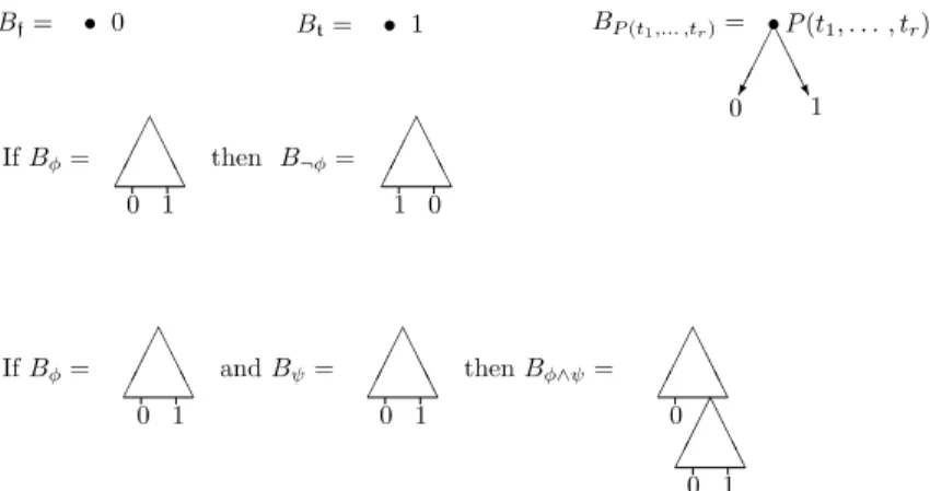
So, a BDD yields, given a structure and a valuation, a true value. As such they can be used to represent formulas. The following definition explains a way to do this. We sometimes use pictures, instead of rather laborious definitions of BDDs, as we think that these are as clear, and far easier to understand. We have adopted the convention to draw outgoing false continuations at the left and outgoing true continuations at the right of a node. We tag the nodes only with their labels and we draw multiple occurrences of the unique node labelled with 0, and similarly for the node labelled with 1.
Definition 3.4. Fig. 1 shows the BDDs,Bf, Bt, BP (t1,...,tr), B¬φ andBφ∧ψ correspond-ing to the formulasf,t, P (t1, . . . , tr),¬φandφ∧ψ.InBφ∧ψ it does not matter which
diagram is put on top and which one is put below.
Note that we divert here from[2]w.r.t. the definition ofBφ∧ψ,where a strict ordering
on the labels of the nodes is maintained. In [2] it is guaranteed that when traversing a BDD from the root to 0 or 1,the labels are run across in a strict ascending order. We introduce
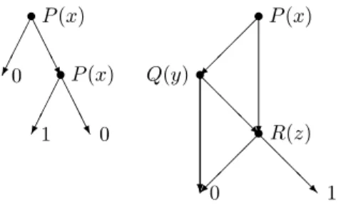
Fig. 2. BDDs forP (x)∧ ¬P (x)and(P (x)∨Q(y))∧R(z).
special rules to sort the labels, as we need these when applying unifiers. As these sorting rules are available anyhow, we have chosen for the simpler presentation of conjunction. As sorting a BDD is a very expensive operation, it seems wise to implement∧on BDDs as is done in [1,2].
Example 3.5. The BDDs belonging to the formulasP (x)∧ ¬P (x)and(P (x)∨Q(y))∧
R(z)are drawn in Fig. 2.
Theorem 3.6. Letφ be a(quantifier free)formula andBφits corresponding BDD. For
each structureAand each valuationζ we find that
A, ζ |=φ iff A, ζ |=Bφ.
Proof. Straightforward on the structure ofφ.
4. Simple operations on BDDs
In this section we provide simple operations to transform BDDs intoreducedor ca-nonical form [2]. We show that the reduced BDDs of (strongly) equivalent formulas are isomorphic (Theorem 4.10) and that the application of simple operators must terminate (Theorem 4.11).
The operatorsNp andJp,q are the same as those in [1], where it is pointed out how
simultaneous application of these two operators can be carried out on a BDD in linear time. Because of the details of the operators are somewhat tricky, we give the definitions in full detail. For easy understanding each operator is depicted.
Definition 4.1 (see Fig. 3). LetB =(Q, l,→f ,→t , s,0,1)be a BDD. Theneglect operator
Np(B)is defined if for someq ∈Q p
t →qandp→f q by: Np l(q) l(q) l(p) A A
l(r) l(p) l(r) l(q) l(p) B A p,q J B A l(s) l(s)
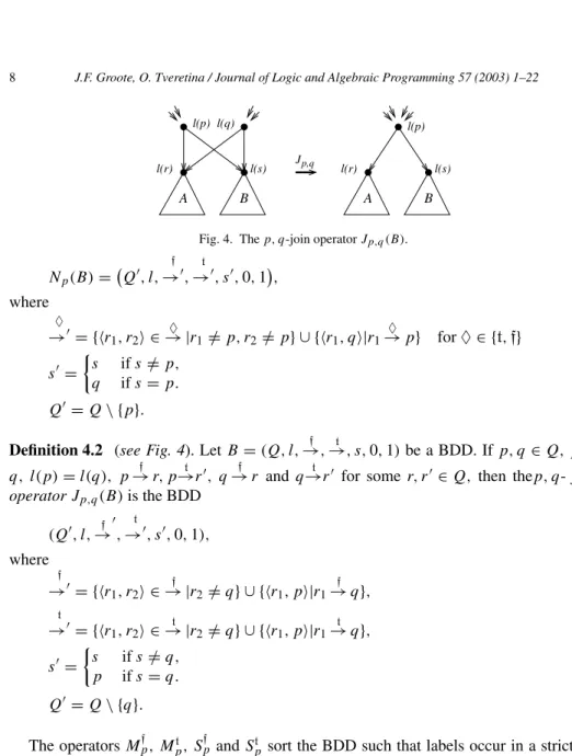
Fig. 4. Thep, q-join operatorJp,q(B).
Np(B)= Q, l, f →, t →, s,0,1, where ♦ → = {r1, r2 ∈→ |♦ r1=/ p, r2=/ p} ∪ {r1, q|r1→♦ p} for♦∈ {t,f} s = s ifs /=p, q ifs=p. Q =Q\ {p}.
Definition 4.2 (see Fig. 4). LetB=(Q, l,→f ,→t , s,0,1)be a BDD. Ifp, q∈Q, p /= q, l(p)=l(q), p→f r, p→t r, q→f r and q→t r for some r, r ∈Q,then thep, q- join operatorJp,q(B)is the BDD (Q, l,→f , t →, s,0,1), where f → = {r1, r2 ∈ f → |r2=/ q} ∪ {r1, p|r1 f →q}, t → = {r1, r2 ∈ t → |r2=/ q} ∪ {r1, p|r1 t →q}, s = s ifs /=q, p ifs=q. Q =Q\ {q}. The operatorsMpf, Mpt, S f
p andSpt sort the BDD such that labels occur in a strict
as-cending order. It is impossible to implement simultaneous application of these operators on a BDD efficiently, as for some polynomial-sized formulas there are exponential-sized BDDs only. When applying the operations on BDDs as described here to propositional logic, the only non-polynomial operator is sorting. It is possible to avoid sorting a BDD, except after application of a unifier.
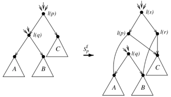
Definition 4.3 (See Fig. 5). LetB=(Q, l,→f ,→t , s,0,1)be a BDD. Ifp, q∈Q, p→f q, andl(p)=l(q),then thef-merge operatorMpf(B)is the BDD
(Q, l, f →,→t , s,0,1), where f → = {r1, r2 ∈ f → |r1=/ p∧r2=/ q} ∪ {p, r|q f →r} Q isQfrom which non-reachable parts are removed.
l(q) l(p) l(q) l(p) B C A f Mp B C A
Fig. 5. Thef-merge operatorMpf(B).
Ifp, q∈Q, p→t qandl(p)=l(q),then thet-merge operatorMt
p(B)is the BDD (Q, l,→f , t →, s,0,1), where t → = {r1, r2 ∈ t → |r1=/ p∧r2=/ q} ∪ {p, r|q t →r} Q isQfrom which non-reachable parts are removed.
Definition 4.4 (See Fig. 6). LetB=(Q, l,→f ,→t , s,0,1)be a BDD. Ifp, q∈Q, p→f q andl(p) > l(q)with respect to the ordering relation>on predicates, then thef-sort oper-ationis defined as follows:
Spf =(Q, l,
t
→,
f
→, s,0,1). Belowp andp are new nodes.
l(r)= l(p) ifr=p, l(q) ifr=p , l(r) otherwise. f → = {r1, r2 ∈ f → |r1=/ porr2=/ p} ∪ {r, p |r f →p} ∪ {p , p} ∪ {p, r|q→t r} ∪ {p, r|q→f r} t → = {r1, r2 ∈ t → |r2=/ p} ∪ {r, p |r t →p} ∪ {p , p} ∪ {p, r|p→t r} Q isQ∪ {p, p }from which parts that become unreachable are removed.
p f S l(s) l(r) l(p) l(q) l(p) l(q) C B A C B A
Ifp, q∈Q, p→t q andl(p) > l(q)with respect to the ordering relation>on predi-cates, then thet-sort operationis defined to be
Spt(B)=(Q, l,
t
→,
f
→, s,0,1). Below,p andp are new nodes.
l(r)= l(p) ifr=p, l(q) ifr=p , l(r) otherwise. f → = {r1, r2 ∈ f → |r2=/ p} ∪ {r, p |r f →p} ∪ {p , p} ∪ {p, r|p→f r} t → = {r1, r2 ∈ t → |r1=/ porr2=/ p} ∪ {r, p |r t →p} ∪ {p , p} ∪ {p, r|q→f r} ∪ {p, r|q→t r}
Q isQ∪ {p, p }from which parts that become unreachable are removed.
Lemma 4.5 (Soundness). Let B be a BDD. We find for p, q∈QB that in case O is
applicable toB O(B)B, whereOis one ofNp, Jp,q, Mpt, M f p, Spt andS f p.
Proof. It is trivial but tedious, to check that for all structuresAand valuationsζ it holds thatA, ζ |=O(B)iffA, ζ |=B.
Definition 4.6. We say that a BDDBisreducedwith respect to some total ordering<on
open predicates iff none of the operatorsNp, Jp,q, Mpt, M
f
p, Spt andS
f
pis applicable toB.
In general the ordering<is not mentioned, assuming it is clear from the context.
The next lemmas work towards Theorem 4.10 saying that strongly equivalent reduced BDDs are unique up to an isomorphism.
Lemma 4.7. LetB, C be BDDs with nodesp∈QB andq ∈QC.LetAbe a structure
and ζ a valuation such that A, ζ |=p and A, ζ |=q. LetP (t1, . . . , tn)be a label not
occurring in the subdags ofBandCrooted withpandq.Then:
1. There exists a structureBand a valuationξsuch that
B, ξ |=p,B, ξ |=qandB, ξ |=P (t1, . . . , tn).
2. There exists a structureBand a valuationξsuch that
B, ξ |=p,B, ξ |=qandB, ξ |=P (t1, . . . , tn).
Proof. ExtendAwith new fresh constants, one for every variable inB, CorP (t1, . . . , tn).
Defineξsuch that it maps every variable to this newly created constant. DefineBto hold on every predicateξ(Q(u1, . . . , um))iffAholds forζ (Q(u1, . . . , um)).Due to the structure
Lemma 4.8. LetB andCbe reduced BDDs. Letp∈QB andq ∈QC such thatpq.
We find:
1. l(p)=l(q), 2. p↓fq↓f, 3. p↓tq↓t,
4. ifBandCare the same BDDs,thenp=q.
Proof. We prove this lemma by contradiction. Assume there are reduced BDDsBandC
containing nodesp∈QB andq∈QCsuch that one of the conditions 1, 2, 3 or 4 do not
hold. Consider such BDDsBandCwith nodesp, qwith minimal value 2|p|+2|q|where
|p|is the length of the longest path leading frompto 0 or 1.
(1) Supposel(p) /=l(q).Consider the case wherel(p) < l(q).The case wherel(p) > l(q)is symmetric, and therefore omitted. As the sort and the merge operator are not ap-plicable toB andC,there are no nodes below p inB and belowq inC labelled with l(p).Now we can show thatp↓fq.The proof of this fact is also by contradiction. As-sumep↓fq.Then, there is a structureAand a valuationζ such thatA, ζ |=p↓f and A, ζ |=q,or vice versa,A, ζ |=p↓f andA, ζ |=q.We only deal with the first case, as the other is almost symmetric. By Lemma 4.7, there is a structureBand a valuationξsuch thatB, ξ|=p↓f,B, ξ |=q andB, ξ|=l(p).Hence,B, ξ |=p.But this contradicts that pq,asB, ξ|=q.So,p↓fq.Similarly, we can show thatp↓tq.Hence, by transi-tivity of , p↓tp↓f.As 2|p↓t|+2|p↓f| 2|p| <2|p|+2|q|it must be thatp↓
t=p↓f,
aspandq were the nodes with smallest exponential distance to end nodes violating one of the properties 1–4 in this lemma. But in this case the neglect operator is applicable, contradicting thatBis reduced. Hence,l(p)=l(q).
(2) Supposel(p)=l(q),butp↓f q↓f.Then there is a structureAand some valua-tionζ such thatA, ζ |=p↓f andA, ζ |=q↓for vice versa,A, ζ|=p↓fandA, ζ |=q↓f. We only consider the first case for symmetry reasons. Asl(p)does not occur in the subdags inBandCrooted withl(p),there is according to Lemma 4.7 a structureBand a valua-tionξ such thatB, ξ |=p↓f,B, ξ|=q↓fandB, ξ |=l(p).Hence,B, ξ |=p,B, ξ|=q contradicting thatpq.
(3) Similar to case 2.
(4) LetBandCbe the same BDDs. Suppose that cases 1–3 hold forpandq.In order to generate a contradiction, assumep /=q.Using 2 and 3,p↓fq↓fandp↓tq↓t.As 2|p↓f|+
2|q↓f|<2|p|+2|q|,it follows thatp↓
f=q↓f.In the same way it follows thatp↓t=q↓t.
Hence the join operator is applicable. But this contradicts thatBis reduced.
Definition 4.9. Let B =(QB, lB, f →B, t →B, sB,0B,1B) and C=(QC, lC, f →C, t →C,
sC,0C,1C)be BDDs. A functionf:QB∪ {0B,1B} →QC∪ {0C,1C}is called a
homo-morphismifflC(f (p))=lB(p), f (p↓f)=f (p)↓f andf (p↓t)=f (p)↓t.In casef is
bijective,f is called anisomorphism. If there exists an isomorphismf:QB∪ {0B,1B} →
QC∪ {0C,1C},thenBandCare calledisomorphic, written asB=C.
Theorem 4.10. Let B and C be reduced BDDs,such that BC. ThenB and C are
isomorphic,i.e.B=C.
Proof. We define functionsf:QB→QCandg:QC→QBas follows:
f (p)=q for theq∈QCsuch thatpq,
Assuming thatf andg are well defined functions, it is easy to see that f is a ho-momorphism using Lemma 4.8. Furthermore,gis clearly the inverse off,provingf an isomorphism.
So, we must only show thatf andgare proper functions. Due to symmetry we only do that forf.AsBC,it follows from Lemmas 4.8.2 and 4.8.3 and the fact that all nodes in Bare reachable from the root that each node inQB is related via to at least one node
inQC.Now, suppose that a nodep∈QBis related to nodesq1, q2∈QC.By transitivity
of it follows thatq1q2.Using Lemma 4.8.4 it must be thatq1=q2.
Theorem 4.11. LetBbe a BDD. The operatorsNp, Jp,q, Mpt, M
f
p, Spt andS
f
pcan only
be applied a finite number of times toB.
Proof. The transformation operators can be formulated as rewrite rules in the following
way (except the join operator), wherel1andl2are predicates withl1> l2. l1(l2(x, y), z)→l2(l1(x, z), l1(y, z)) Spf
l1(x, l2(y, z))→l2(l1(x, y), l1(x, z)) Spt
l1(x, x)→x Np
l1(l1(x, y), z)→l1(x, z) Mpf
l1(x, l1(y, z))→l1(x, z) Mpt
To each DAG we can obtain its canonical tree by undoing the sharing of subdags. Using a recursive path ordering [4,8], it is straightforward to see that application of these rules must terminate on these trees.
If the rules are applied on DAGs, observe that each rewrite of the DAG corresponds to one or more rewrites of the canonical tree. So, rewriting the DAG must also terminate.
Repeated application of the join operator must also terminate, as the number of nodes is strictly decreasing. The application of the Join operator does not change the canonical tree of a BDD. Therefore, it does not enable more rewrite steps to be applied. Hence, repeated application of all operators must terminate.
Notation 4.12. LetBbe a BDD and letCbe a reduced BDD such thatBC.According
to Theorem4.10C is unique up to an isomorphism. According to Theorem4.11C must exist,and can be effectively obtained. This allows us to writeR(B)forC.
Note that Theorem 4.10 implies thatR(Bφ)=Btifφis strongly equivalent to a
tautol-ogy. Note also thatR(Bφ)=Bfifφis strongly equivalent to a contradiction. This
obser-vation is the basis for using BDDs for propositional logic. Contrary to what is stated in [2], due to the different setting it is not the case thatR(Bφ)is the smallest representation forφ.
This is due to the particular construction of conjunction on BDDs and the sorting operator that can cause BDDs to grow.
5. Advanced operations on BDDs
In this section we present two operators on BDDs that are solely defined for predicate logic. The first one is acopying operatorC(B)that putsBin conjunction with a copy of itself, where variables are made fresh.
The second operator is theunification operatorUζ(B)whereζ is a so-calledrelevant
unifier.Uζ(B)instantiatesBaccording toζ.
Definition 5.1. LetBbe a BDD in which variablesxoccur. Thecopy operatorC(B)is
defined as
C(B)=B∧B[x:= x1],
wherex1is a sequence of pairwise distinct variables not occurring inB.
Definition 5.2. LetP (t1, . . . , tn), Q(u1, . . . , um)∈P(P r, F, V ).A substitutionζ:V →
T(F, V ) is called a unifier of P (t1, . . . , tn) andQ(u1, . . . , um) iff ζ (P (t1, . . . , tn))=
ζ (Q(u1, . . . , um)).A unifierζ ofP (t1, . . . , tn)andQ(u1, . . . , um)is calledmost general
if for each unifierζ ofP (t1, . . . , tn)andQ(u1, . . . , um)there is a substitutionξsuch that
ξ◦ζ =ζ .
If predicatesP (t1, . . . , tn)andQ(u1, . . . , um)are unifiable, then they have a MGU,
which is unique modulo renaming of variables. There is also an MGU that is idempotent, i.e.ζ (ζ (x))=x.Moreover, the MGU can be determined in linear time [10,11].
Definition 5.3. LetB =(Q, l,→f ,→t , s,0,1)be a BDD and letζ be a substitution. The BDDζ (B)is defined as:
ζ (B)=(Q, λx.ζ (l(x)),→f ,→t , s,0,1).
In the following definition we definerelevant unifiers. This definition and Lemma 5.5 help us to see that relevant unifiers are easy to find in reduced BDDs.
Definition 5.4. LetB=(Q, l,→f ,→t , s,0,1)be a BDD. A nodep∈Qis called redun-dantifp↓tp↓f.
A path
p0−→♦0 p1−→ · · ·♦1 ♦n− 1
−→pn−→♦n 2
for2∈ {0,1}is calledallowedif there are no 0i < jnsuch thatl(pi)=l(pj)and
♦i =/ ♦j.
A nodep∈Qis calledtrue–true capableif there is an allowed path p→t p1♦
1
→ · · ·♦n−1
→ pn→♦n1
A substitutionζ is called arelevant unifier forBif there is a path p0→♦0p1→ · · ·♦1 ♦n−
1
→ pn→♦n1
withp0=s; for all 0in pi is not redundant; for some 0i, jn♦i =f,♦j =t
andζ is an idempotent MGU ofl(pi)andl(pj).
Lemma 5.5. LetBbe a reduced BDD. We find:
• There are no redundant nodesp∈QB.
• Ifpi is not true–true capable,pi↓t=0.
• ζ is a relevant unifier forBiff for some0i, jn♦i =f,♦j =tandζis the MGU
ofl(pi)andl(pj)on the rightmost path
p0→♦0p1→ · · ·♦1 ♦n− 1
→ pn→♦n1
ofB. Proof
• SupposeBis reduced and there is a redundant nodep∈QB.Hence,p↓tp↓f.
Ac-cording to Lemma 4.8.4p↓t =p↓f.Hence, the neglect operator is applicable, con-tradicting thatBis reduced.
• If a path inB would not be allowed, the sort and/or merge operators are applicable, contradicting thatBis reduced.
• Ifpiis not true-true capable, every path starting withp↓tends in 0. Clearly, ifpi↓t =/ 0
the neglect operator is applicable at the one but last node on a path starting inp↓t.This contradicts thatBis reduced.
• We can only turn left on a non-true-true preserving node on the path where we search for relevant unifiers. According to the previous items in this way we walk along the rightmost path ofBto 1.
It is obvious from this characterization that relevant unifiers are easy to find as we only need to inspect the rightmost path ofB.For instance in the BDD at the left of Fig. 7 on page 18 the only relevant unifier on the rightmost path to 1 isy:=a.And in the BDD in Fig. 10 on page 19 the only relevant unifier on the rightmost path isy:=d.
Definition 5.6. LetBbe a BDD. Theunification operatorUζ(B)is defined by
Uζ(B)=ζ (B) ifζ is a relevant unifier ofB.
Note that ifζ is a relevant unifier, thenUζ(B)contains strictly less variables thanB.
Lemma 5.7(Soundness). LetBbe a BDD.
• B≈C(B),
• B≈B∧Uζ(B).
Proof. Easy logical consequence.
6. Completeness
In this section we show that if a formulaφis unsatisfiable, then there is a sequence of operators onBφthat turns it intoBf.The first lemma attracts attention to rightmost paths
in BDDs for calculating relevant unifiers. The next lemma shows that ifBφ is strongly
equivalent toBf then we can find it by repeatedly applying relevant unifiers onBφ.
Theo-rem 6.3 says, using Herbrand’s theoTheo-rem that ifBφis unsatisfiable we must apply relevant
unifiers to a certain number of copies toB,all interleaved with reduction operators. The algorithm in Section 7 is nothing more than recursively searching for this sequence of operators.
Lemma 6.1. LetB=(Q, l,→f ,→t , s,0,1)be a reduced BDD andξa closed substitution such thatξ(B)Bf.If there is a rightmost(allowed)path
q0−→♦0 q1−→ · · ·♦1 ♦m− 1
−→qm−→♦m 1
withq0=B↑,then there are0i, jmwith♦i =f,♦j =tandξ(l(qi))=ξ(l(qj)).
Proof. Let
s=q0−→♦0 q1−→ · · ·♦1 ♦m− 1
−→qm−→♦m 1
be the rightmost (allowed) path inB. Suppose there are no 0i, j m with♦i =f,
♦j =tandξ(l(qi))=ξ(l(qj)).Then, we can construct a Herbrand structureAHsuch that
AH, ξ |=B.
Define the relations inAHsuch that for each nodeqi:
[[l(qi)]]AξH =
0 if♦i =f
1 if♦i =t
and take[[l(qi)]]AξH =0 elsewhere.
As for 1i, jm,♦i =f,♦j =t,impliesξ(l(qi)) /=ξ(l(qj)),the definition ofAH
is indeed correct. Now it is trivial to check thatAH, ξ |=B,contradicting thatξ(B)Bf,
asAH, ξ |=Bf.
Lemma 6.2. Let B=(Q, l,−→f ,−→t , s,0,1)be a reduced BDD andξ a substitution
such thatξ(B)Bf.Then there is a sequence of relevant unifiersζ1, . . . , ζnsuch that
R(Uζ1(R(Uζ2(. . . (R(Uζn(B)))))))=Bf.
Moreover, nis smaller or equal than the number of variables inB.
Proof. We apply induction on the number of variables that occur inB.Note that if there
are no variables inB, ξ(B)=B,and therefore,BBf.Hence, asBis reduced,B =Bf.
So, we can take the sequence of relevant unifiers to be empty.
If there arek >0 variables inB,we know there is an allowed path to 1 inB,as oth-erwiseBBf,and using the same reasoning as above, we take the sequence of relevant
unifiers to be empty. As there is an allowed path to 1 inB then according to Lemma 6.1 there is also a rightmost allowed path
q0 ♦ 0
−→q1−→ · · ·♦1 ♦m− 1
−→qm−→♦m 1
to 1 in B with q0=B↑, and some 0i, j mwith ♦i =f, ♦j =t and ξ(l(qi))=
ξ(l(qj)).Hence, there is a relevant unifierζ such thatζ (l(pi))=ζ (l(pj)).Note that in
Uζ(B)there are strictly less variables than in B. As the operator R does not introduce
new labels of nodes, R(Uζ(B)) also contains strictly less variables than B. Moreover,
as, due to the fact that ζ is an mgu, there is some substitution ξ such that ξ ◦ζ = ξ.So,ξ (R(Uζ(B)))Bf.Furthermore,R(Uζ(B))is reduced. Now using the induction
hypothesis, there must be a sequenceζ1, . . . , ζnsuch that
R(Uζ1(. . . (R(Uζn(R(Uζ(B)))))))=Bf. So,ζ1, . . . , ζn, ζ is the required sequence.
Theorem 6.3. LetBbe an unsatisfiable BDD. Then
R(Uζ1(. . . R(Uζn(
ktimes
R(C(. . . R(C(B))))))))=Bf for certainn, k0and relevant unifiersζ1, . . . , ζn.
Proof. AsBis unsatisfiable, it follows from Theorems 2.5 and 3.6 that there are closed
substitutionsξ1, . . . , ξmsuch that m
i=1
ξi(B)Bf.
Select someksuch that 2k m.The term (ξ1◦ι[ x1:=x]) . . . (ξm◦ι[ xm:=x])(
ktimes
C(C(. . . (C(B)) . . .)))Bf. (1)
Here, the notationι[ xi:=x]is a renaming that takes care that the substitutionξioperates
on the appropriate variables. Writeξ =(ξ1◦ι[ x1:=x]) . . . (ξm◦ι[ xm:=x]).According to
Lemma 4.5R(B)B.So, we may interleave the copying operators with simple reduction operators without changing strong equivalence. Write
B = ktimes R(C(. . . (R(C(B)) . . .))) . Rephrasing (1) yields ξ(B)Bf.
By Lemma 6.2 it follows that there are relevant unifiersζ1, . . . , ζmsuch that
R(Uζ1(. . . (R(Uζm(B)))))=Bf. which is exactly what we must show.
7. Algorithm
The previous lemma suggest the following algorithm to find out whether a formulaφis unsatisfiable: Solve(φ)= B: =R(Bφ) Repeat TryToReduce(B) B: =R(C(B)) Endrepeat TryToReduce(B)=
IfB =Bf,report ‘unsatisfiable’ andstop
For all relevant unifiersζ ofBTryToReduce(R(Uζ(B)))
It says that firstR(Bφ)should be constructed. As is shown in [1,2] this can be done
up. The depth is linearly bounded by the number of different predicates). Note that if the construction is carried out as described in [1,2] the expensive sorting operator is not applied.
Then, recursively, relevant unifiers are applied toB inTryToReduce(B).Finding the relevant unifiers can be done efficiently. All pairs of pi, pj of predicates labelling the
rightmost pathσofB,withpi↓t =0 andpj↓t=/ 0 must be examined. Hence, if the length
ofσ isl,there are at most(1/4)l2potentially unifiable predicates. Using the algorithms proposed by [10,11] unifiers can be found linearly in the size of the terms.
Application of the unifier, calculation ofR(Uζ(B))may be costly. It is linear to
cal-culateUζ(B).But this may destruct the ordering of the labels. When reducing, it may be
necessary that the costly sorting operators are applied. An attempt can be made to avoid extensive sorting by grouping predicates with the same predicate symbol together.
Also the recursive nesting of calls toTryToReducecould be a cause of inefficiency. However, at each call at least one variable is instantiated. Therefore, the depth of recursive calls toTryToReduceis limited by the number of free variables in the BDD.
WhenTryToReduce(B)does not yieldBt,then a copy must be made, i.e. the command
B:=R(C(B))is carried out. The copy operator is defined using the∧and hence, using the techniques in [1,2]R(C(B))can be calculated efficiently.
So, the programme is clearly browsing through larger and larger BDDs of the form
R(Uζ1(R(Uζ2(. . . R(C(. . . R(C(Bφ)))))))) (2)
where we stop if this BDD appears to beBf.If φ is unsatisfiable, this algorithm must
terminate according to Theorem 6.3. Moreover, if we find that (2) is equal toBf then we may conclude with Lemmas 4.5 and 5.7 thatBφ≈Bφ∧Bf,which means thatBφmust be
unsatisfiable.
Note that the algorithm presented here only sketches a basic approach on which a num-ber of improvements are possible. First, it is sometimes possible to identify that a formula is satisfiable in an early phase of the protocol. This for instance seems to happen if finding unifiers fails. It is also the case that sometimes redundant unifiers are calculated in the approach above, for instance unifiers that undo a copying step. In [6] it has been described how to avoid some of the computational overhead.
8. Examples
In this section we apply the proposed method to three examples taken from [12]. The first one is chosen for its simplicity, while it still expresses an interesting fact. The second one is chosen because it needs copying and the third one is interesting because it is rated as reasonably difficult, while it is still small enough to carry out the construction of the BDD and the calculation of relevant unifiers by hand.
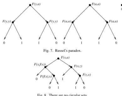
8.1. Russel’s paradox
Problem 39 of [12] says that ‘there is no Russell set’, i.e. a set which contains exactly those sets which are not members of themselves. The predicateF (x, y)must be read as ‘x is a member ofy’. The problem is originally stated as
F(y,y) F(y,y) F(y,a) F(a,a) F(a,a) F(a,a) 0 1 1 0 1 1 0 0 0
Fig. 7. Russel’s paradox.
1 1 0 0 F(x,f(x)) F(x,a) F(x,z) F(z,x) F(f(x),x) 1 0
Fig. 8. There are no circular sets.
We negate and Skolemise the formula. After removal of the remaining universal quan-tifier we obtain
F (y, a)↔ ¬F (y, y) (4)
whereais a Skolem constant. The leftmost BDD in Fig. 7 is obtained from this formula. There is one relevant unifier, which is obtained by making a rightmost walk through the BDD to an endnode 1.On this path the predicatesF (y, a)andF (y, y)are unifiable, with unifierζ (y)=a.Applying the unifier to this BDD yields the BDD in the middle of Fig. 7. Reduction leads toBf(at the right in Fig. 7) showing that (4) is unsatisfiable, and hence
(3) a tautology.
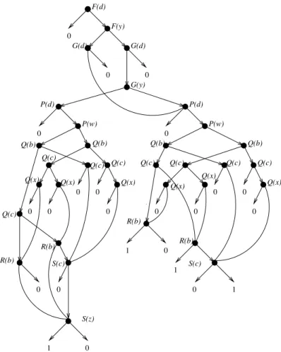
8.2. There are no circular sets
The second example is problem 42 of [12]. It says that ‘a set is circular if it is a member of another set, which in turn is a member of the original’. We show that there is no set containing all non-circular sets. The original formulation of this theorem is
¬∃y∀x(F (x, y)↔ ¬∃z(F (x, z)∧F (z, x))). (5) 0 0 F(x,f(x)) F(x,a) F(x,z) F(z,x) F(f(x),x) 0 1 1 0 0 1 F(u,a) F(u,v) F(v,u) F(f(u),u) F(u,f(u)) 0 0 1 1 0 1 F(u,a) F(u,v) F(v,u) F(f(u),u) F(u,f(u)) 0 0 0 F(a,a) 0 F(a,f(a)) F(f(a),a)
1 0 1 G(y) P(d) P(w) Q(b) Q(c) Q(x) P(w) Q(c) Q(x) R(b) Q(x) Q(c) F(d) F(y) G(d) R(b) R(b) Q(b) Q(c) Q(c) Q(c) Q(x) Q(x) Q(x) Q(b) Q(c) S(c) Q(c) 0 0 0 0 0 0 0 0 0 0 0 0 0 0 P(d) Q(b) R(b) 0 1 S(c) G(d) 0 0 0 S(z) 0 1
Fig. 10. A tedious problem from monadic logic.
Negation, Skolemisation and removal of quantifiers yields (F (x, a)−→ ¬(F (x, z)∧F (z, x)))∧(¬(F (x, f (x))
∧F (f (x), x))−→F (x, a)). (6)
Obviouslyaandf are Skolem functions. Note that the structure of the formula has changed somewhat due to Skolemisation, as in (5) there is a quantifier in the scope of a↔.In Fig. 8 the BDD for (6) is depicted. There are two relevant unifiers, the first one mappingzand xtoa,and the second one mappingxtoz.Application of the first unifier leads to a BDD B that neither is equal toBf nor has another relevant unifier. Application of the second
unifier leads to a subsequent unifier, mappingztoa.In effect application of this unifier leads again to the BDDB.In this way the BDDBfcannot be obtained.
According to the algorithm we now must apply the copying operator. This leads to the BDD at the left of Fig. 9. We have used fresh variablesuandvfor respectivelyx andz. Along a rightmost walk in this tree we obtain the following six unifiers.
x:=a z:=a x:=v u:=a z:=x u:=a v:=a u:=z x:=a v:=u
0 F(d) S(z) S(c) 1 0 0 1 0 0 0 R(b) G(d) 0 Q(b) P(d) 0 0 0 0 0 0 Q(c) S(c) Q(c) Q(b) Q(x) Q(c) Q(x) R(b) Q(x) Q(c) P(w) 0 Q(c) 0 0 0 0 Q(b) R(b) 0 Q(c) Q(x) Q(b) 0 F(d) G(d) 0 P(d) 0 P(w)
Fig. 11. A tedious problem from monadic logic (continued I).
If we apply the first one to the BDD we obtain the BDD on the right-hand side of Fig. 9. Now we find the following unifiers along the rightmost walk.
u:=f (a) v:=a u:=f (a) v:=a u:=a u:=a v:=a u:=v
Applying the first unifier yields a BDD that reduces toBf.So, formula (6) is
unsatisfi-able and hence, formula (5) is a contradiction.
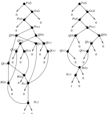
8.3. A problem for monadic logic
Some problems (i.e. problems 34, 47, 69 and 70) in [12] are rated as more difficult. They cannot be solved manually due to their length. In this example we apply our BDD techniques to problem 28, which is rated among the hardest ones. The hardest problem among the more tedious monadic logic problems from Kalish and Montague’ is formulated as follows. Note that there is a small mistake in its formulation in [12], as mentioned in the related Erratum. ((∀x(P (x)−→ ∀xQ(x)))∧ (∀x(Q(x)∨R(x))−→ ∃x(Q(x)∧S(x)))∧ (∃xS(x)−→ ∀x(F (x)−→G(x))))−→ ∀x (P (x)∧F (x)−→G(x)) (7)
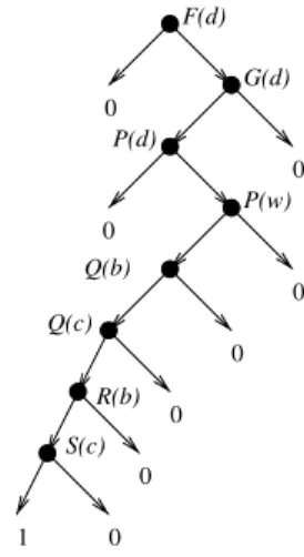
1 0 0 S(c) 0 R(b) Q(c) 0 0 Q(b) 0 F(d) G(d) 0 P(d) 0 P(w)
Fig. 12. A tedious problem from monadic logic (continued II).
By denying and Skolemising the formula, we obtain (a, b, canddare Skolem constants andw, x, yandzare variables):
(P (w)−→Q(x))∧
((Q(b)∨R(b))−→(Q(c)∧S(c)))∧ (S(z)−→(F (y)−→G(y)))∧ (P (d)∧F (d)∧ ¬G(d))
(8)
The BDD of this formula is depicted in Fig. 10. Its labels are sorted alphabetically. It has 35 nodes. The BDD has only one relevant unifier,y:=d.Application of this unifier reduces the size of the BDD with almost 50%. The newly obtained BDD is depicted on the left of Fig. 11. Again, it has only one relevant unifier, beingz:=c.The BDD resulting after application of this unifier has been depicted on the right-hand side of Fig. 11. This last BDD has two relevant unifiers,x:=bandx:=c.After applying either of those it we obtain the BDD depicted in Fig. 12. This BDD has the unique relevant unifierw:=d.Application of this last unifier yields the BDDBf,showing (8) unsatisfiable, and hence (7) a tautology.
9. Conclusions
We have designed a way to apply BDDs to predicate logic. We have shown that this yields a complete proof procedure. The procedure works by computing a Herbrand con-junction: if a quantifier-free formula is unsatisfiable then there exists a finite conjunction of ground instances of the formula that is propositionally inconsistent. If the proof has failed with a given number of copies a variant of the initial formula is conjunctively added.
We have shown that for the examples we have considered the technique leads so quickly to results that they can be carried out by hand. We have not implemented the system and hence not tried to use it on larger examples.
Independently of the work reported in here two other groups have been working on extending BDDs to predicate logic [5,6,14,15] in a rather similar way, probably indicating the naturalness of the approach.
In [14,15] the ideas have been implemented by transforming a BDD into a PROLOG programme. The PROLOG programme takes care of finding the unifiers, that in this case are found on the leftmost path (instead of on the rightmost path as has been done here). The implemented system is called SHARE and is available by contacting the author [16]. It is interesting to know that SHARE solved problem 1–46 of Pelletier [12] without men-tionable problems (see [14]).
Acknowledgements
We thank Jaco van de Pol and Hans Zantema for their assistance in proving termination of the basic operators on BDDs. We also thank Jaco van de Pol for his detailed comments, that contributed considerably to the quality of this paper. Thanks also go to Jean Goubault, Joachim Posegga and Bas van Vlijmen for general discussion and comments.
References
[1] K.S. Brace, R.L. Rudell, R.E. Bryant. Efficient implementation of a BDD package. 27th ACM IEEE Design Automation Conference 1990, pp. 40–45.
[2] R.E. Bryant, Graph-based algorithms for boolean function manipulation, IEEE Trans. Comp. C-35 (8) (1986) 677–691.
[3] J.R. Burch, E.M. Clarke, K.L. McMillan, D.L. Dill, L.J. Hwang, Symbolic model checking 1020states and beyond, Inform. Comput. 98 (2) (1992) 142–170.
[4] N. Dershowitz, Termination of rewriting, J. Symbol. Comput. 3 (1) (1987) 69–116.
[5] J. Goubault, Syntax independent connections, in: D. Basin, B. Fronhöfer, R. Hähnle, J. Posegga, C. Sch-wind (Eds.), Proceedings of the 2nd Workshop on Theorem Proving with Analytic Tableaux and Related Methods, 1993.
[6] J. Goubault, Proving with BDDs and control of information, unpublished manuscript, 1995.
[7] J.F. Groote, H. Zantema, Resolution and binary decision diagrams cannot simulate each other polynomially, Technical Report UU-CS-2000-14, Department of Computer Science, Utrecht University, 2000.
[8] J.W. Klop, Term rewriting systems, in: S. Abramsky, D.M. Gabbay, T.S.E. Maibaum (Eds.), Handbook of Logic in Computer Science, vol. 2, Oxford Science Publications, 1992, pp. 1–116.
[9] K.L. McMillan, J. Schwalbe, Formal verification of the Gigamax cache consistency protocol, in: Interna-tional Symposium on Shared Memory Multiprocessing, 1991.
[10] A. Martelli, U. Montanari, An efficient unification algorithm, ACM Trans. Prog. Lang. Syst. 4 (2) (1982) 258–282.
[11] M.S. Paterson, M.N. Wegman, Linear unification, J. Comp. Syst. Sci. 16 (1978) 158–167.
[12] F.J. Pelletier, Seventy-five problems for testing automated theorem provers, J. Automat. Reason. 2 (1986) 191–216. Journal of Automated Reasoning, 4 (1988) 235–236 (See also Errata).
[13] J. Possega, B. Ludäscher, Towards first-order deduction based on Shannon graphs, in: Proceedings of 16th German Conference on AI(GWAI-92), volume 671 of Lecture Notes in Artificial Intelligence, Springer-Verlag, 1992, pp. 67–76.
[14] J. Posegga, P.H. Schmitt, Automated deduction with shannon graphs, J. Logic Comput. 5 (6) (1995) 697– 729.
[15] J. Posegga, K. Schneider, Deduction with first-order BDDs, in: D. Basin, Bertram Fronhöfer, Reiner Häh-nle, J. Posegga, C. Schwind (Eds.), Proceedings of the 2nd Workshop on Theorem Proving with Analytic Tableaux and Related Methods, 1993.
[16] J. Posegga, SHAnnon graph REfutation system. This is an implementation of a BDD based theorem prover. Information: [email protected], 1995.