Optimal ordered binary decision diagrams for
read-once formulas
Martin Sauerho
a;∗;1, Ingo Wegener
a;1, Ralph Werchner
a aFachbereich Informatik, Universitat Dortmund, 44221 Dortmund, Germany Received 16 January 1998; received in revised form 3 August 1999; accepted 9 August 1999Abstract
In many applications like verication or combinatorial optimization, ordered binary decision diagrams (OBDDs) are used as a representation or data structure for Boolean functions. Ecient algorithms exist for the important operations on OBDDs, and many functions can be represented in reasonable size if a good variable ordering is chosen. In general, it is NP-hard to compute optimal or near-optimal variable orderings, and already simple classes of Boolean functions contain functions whose OBDD size is exponential for each variable ordering. For the class of Boolean functions representable by fan-in 2 read-once formulas the structure of optimal variable orderings is described, leading to a linear time algorithm for the construction of optimal variable orderings and the size of the corresponding OBDD. Moreover, it is proved that the hardest read-once formula has an OBDD size of order nÿ where ÿ= log
4(3 +
√
5)¡1:1943. ? 2000 Elsevier Science B.V. All rights reserved.
Keywords:Ordered binary decision diagram; Ecient algorithms; Boolean function; Variable ordering; Read-once formula
1. Introduction
In order to work with Boolean functions one needs a representation or data structure which has small size for “many” Boolean functions and which supports the ecient realization of important operations on these functions. Within the more than 10 years since their introduction by Bryant [4], OBDDs have become the state-of-the-art repre-sentation in many applications.
The survey article [5] describes applications in CAD tools for verication, synthe-sis and analysynthe-sis of combinatorial and sequential circuits, and automatic test pattern
∗Corresponding author.
E-mail addresses: [email protected] (M. Sauerho), [email protected] (I. Wegener), [email protected] (R. Werchner)
1Supported by DFG grant We 1066/8-2.
0166-218X/00/$ - see front matter?2000 Elsevier Science B.V. All rights reserved. PII: S0166-218X(99)00210-3
generation. But OBDDs have also found applications in combinatorial optimization problems like maximum ow [12] or counting problems like determining the number of knight’s tours on an 8×8-chessboard [16]. Hence, it is well motivated to investigate OBDDs from a complexity theoretical and mathematical viewpoint.
In the following, we dene OBDDs as a restricted type of branching programs.
Deÿnition 1. A branching program on n variables is a directed acyclic graph with one source. Each sink is labeled by a Boolean constant and each other node v by a Boolean variable from {x1; : : : ; xn}. Such a nodevhas two outgoing edges, one labeled by 0 leading to the node low(v) and the other labeled by 1 and leading to the node high(v). The branching program represents the Boolean function f: {0;1}n → {0;1} dened in the following way. An edge with label c ∈ {0;1} leaving a node labeled by xi is activated by an input a ∈ {0;1}n if ai =c. The value f(a) is dened as the value of the sink reached by the unique path of edges activated by a which starts at the source. The size of a branching program is the number of its non-terminal nodes.
A branching program is called read-once if each path contains at most one node labeled by xi for each variable xi. A variable ordering of n variables is a permu-tation of {1;2; : : : ; n} which we also describe by the permuted variable sequence
x(1); : : : ; x(n). An ordered binary decision diagram (OBDD) with respect to the vari-able ordering (-OBDD for short) is a read-once branching program where the labels of the successors of a node vare located behind the label of v in the sequence
x(1); : : : ; x(n).
It is well known [4] that the OBDD of minimal size (called reduced OBDD) is unique for a given function and a xed variable ordering. By an optimal variable ordering for a given function we mean an ordering which leads to the reduced OBDD of the smallest possible size representing this function.
The following two problems are essential for the application of OBDDs. Which classesCof Boolean functions completely consist of functions which have polynomial-size OBDDs and how can we estimate the OBDD polynomial-size of all functions in C? For which classesC is it possible to compute an optimal or near-optimal variable ordering eciently?
Already very small classes of Boolean functions like the class of functions with polynomial-size DNFs (disjunctive normal forms) contain functions which have expo-nential OBDD size for each variable ordering. In [26], the OBDD size of symmetric Boolean functions on n variables is described by structural properties: All symmet-ric Boolean functions have an OBDD size of O(n2) and there are symmetric functions which need size (n2). These results have been generalized to some classes of partially symmetric Boolean functions [25].
Obviously, it is NP-hard to compute an optimal variable ordering if the function is described by a circuit. The problem even is NP-hard [3] if the function is already described by an OBDD. Recently, it has been shown that it is also NP-hard to compute
an almost optimal variable ordering in this situation [22,23]. Consequently, a lot of heuristics for the computation of variable orderings have been proposed for practical applications of OBDDs [7–9,17,19]. These algorithms are also used to generate initial orderings for iterative improvement techniques [2,10,14,18,20,21].
In this article, we answer the questions posed above for the class of Boolean func-tions representable by fan-in 2 read-once formulas.
Deÿnition 2. A read-once formula on n variables x1; : : : ; xn is a binary tree with n leaves labeled by x1; : : : ; xn. The inner nodes (also called gates) are labeled by func-tions from B∗
2, by which we denote the set of all Boolean functions on two vari-ables (AND, OR, NAND, NOR, xy; xy; x∨y,x∨y, EXOR, NEXOR). A read-once formula represents the Boolean function f:{0;1}n → {0;1} which is computed by recursively applying the functions at the inner nodes to the functions or variables at their children.
The classes of Boolean functions representable by dierent kinds of read-once for-mulas have been frequently investigated as natural classes of Boolean functions, e.g., in the setting of algorithmic learning. Angluin and Hellerstein [1] have considered the problem of learning read-once formulas over the restricted basis {AND, OR, NOT}, while Bshouty et al. [6] have proved similar results even for read-once formulas over the basis of arbitrary Boolean functions with constant fan-in and the basis of arbitrary symmetric Boolean functions. Heiman et al. [13] have investigated the randomized decision tree complexity of read-once formulas of constant depth over the basis of threshold functions. In this paper, we always consider read-once formulas over the basis of all Boolean functions with fan-in 2 as dened above.
There is no heuristic for the computation of good variable orderings which computes an optimal variable ordering for OBDDs representing an arbitrary read-once formula according to the above denition. Moreover, for read-once formulas like x1x2∨x3x4∨ · · ·∨xn−1xn it is easy to prove that the optimal variable ordering leads to an OBDD of linear size while all but an exponentially small fraction of all variable orderings lead to OBDDs of exponential size [28]. Hence, the considered problems are not trivial for the class of read-once formulas.
In Section 2, we state some denitions and basic facts. Then we consider variable orderings which can be obtained by a depth-rst search (DFS) traversal of the tree corresponding to the read-once formula. For such so-called DFS variable orderings we completely describe the structure of reduced OBDDs in Section 3. In Section 4, we then prove that for functions representable by a read-once formula there always exists an optimal variable ordering which is a DFS variable ordering. These results lead to an algorithm which from a read-once formula computes an optimal variable ordering and the size of the corresponding OBDD in linear time with respect to the number of variables (Section 5). The corresponding OBDD can be computed in linear time with respect to its size. In Section 6, we nally prove our mathematically most involved result, namely an upper bound of 1:36nÿ on the size of optimal OBDDs for read-once
formulas, where ÿ= log4(3 +√5)¡1:1943. Hence, all these functions have OBDDs of small polynomial size. This upper bound is asymptotically optimal. We present a sequence of read-once formulas which have an optimal OBDD size which for innitely many n is larger than 1:33nÿ.
2. Further deÿnitions and basic facts
In this section, we review some further denitions and basic facts on OBDDs. For our proofs, it is essential to describe which functions are represented at the nodes of reduced OBDDs. A function f is said to depend essentially on a variable xi if the subfunctions (cofactors) f|xi=0 and f|xi=1 are not equal. The proof of the following theorem describing the structure of OBDDs is due to Sieling and Wegener [24].
Theorem 3. Let f:{0;1}n → {0;1} be deÿned on the variables x
1; : : : ; xn. The re-duced OBDD forf and the variable ordering= id contains as manyxi-nodes(i.e.; nodes labeled by variable xi) as there are dierent subfunctionsf|x1=a1;:::;xi−1=ai−1; for
a1; : : : ; ai−1 ∈ {0;1}; which depend essentially onxi.
We will now introduce two extensions of the denition of OBDDs from the last section.
First, we allow that a single OBDD may represent several Boolean functionsf1; : : : ; fr. Such an OBDD may have up to r sources. For each fi, there is a pointer (labeled by the name of the function) to a node of the graph which represents this function in the way described in Denition 1. For a xed set f1; : : : ; fr of functions, the reduced OBDD representing these functions is unique. The number of nodes of this reduced OBDD labeled by a xed variable is obtained by counting subfunctions of f1; : : : ; fr analogous to Theorem 3. OBDDs representing several functions are also known as
SBDDs, shared OBDDs, and have been introduced by Minato et al. [19].
We use the notation size(f1; : : : ; fr; ) for the size of the reduced OBDD with vari-able ordering which simultaneously represents f1; : : : ; fr. By size(f1; : : : ; fr) we de-note the minimum of the sizes of OBDDs for f1; : : : ; fr over all variable orderings.
In practice, one usually works with OBDDs containing complemented edges which have also been introduced by Minato et al. [19].
Deÿnition 4. An OBDD with complemented edges has the same structure as a usual OBDD, but each edge in the graph carries an additional complement label which is either 0 or 1. This holds for edges between nodes of the OBDD as well as for the pointers belonging to each represented function. In order to evaluate a function f
represented by such an OBDD for an input a, one starts at the node which represents
f and follows the unique path of edges activated by a. The output f(a) is obtained by computing the parity of the label of the sink nally reached and all complement labels on the path, including that of the pointer for f.
In order to obtain a unique representation for a xed set of functions, one imposes the restriction on OBDDs with complemented edges that only edges to low-successors may carry the complement label 1 and that the 1-sink is the only sink. We use the name
OBDDs with complemented edges in canonical form for this type of representation. We denote the size of reduced OBDDs with complemented edges in canonical form by sizece. The following theorem describes the structure of these OBDDs.
Theorem 5. Let f be deÿned on the variables x1; : : : ; xn. Let G be the reduced
-OBDD with complemented edges in canonical form which represents f; where
= id. The number of xi-nodes in G is exactly half the number of xi-nodes in the reduced-OBDDG0 which represents(f;f).Especially;it holds that size(f;f; ) = 2 sizece(f; ).
Proof. Let f1; : : : ; fr denote the dierent subfunctions f|x1=a1;:::;xi−1=ai−1 depending
es-sentially on xi. If we construct the xi-level of the reduced -OBDD G with comple-mented edges, we can save the node forf‘, if for somek ¡ ‘, we havefk= f‘. Hence, we getr−snodes ifsis the number of indices ‘ such thatfk= f‘, for somek ¡ ‘. If we construct the xi-level of the reduced -OBDD G0 for (f;f), we can start with 2r nodes for f1; : : : ; fr;f1; : : : ;fr. We can save a node if fk= f‘. But then also f‘= fk. Hence, we can save 2s nodes, and the number of xi-nodes in G0 is 2r−2s= 2(r−s), i. e., twice the number of xi-nodes in G.
In the following, we will usually talk about OBDDs without complemented edges. We will use the above theorem later on to transfer our results for usual OBDDs without complemented edges to OBDDs with complemented edges.
As already mentioned in the introduction, variable orderings of the following special type will play a major role for this paper.
Deÿnition 6. A variable ordering is called a DFS variable ordering for a read-once formula if there is a depth-rst traversal of the tree corresponding to the formula which generates a list of variables describing this ordering as its output. During the traversal, the order of successors may be chosen arbitrarily for each non-terminal node.
3. The structure of OBDDs for read-once formulas and DFS variable orderings
Let an arbitrary read-once formula representing a Boolean function f be given. We assume that f is of the form
f(x1; : : : ; xk; y1; : : : ; ym) =g(x1; : : : ; xk)⊗h(y1; : : : ; ym):
In the tree corresponding to the read-once formula, ⊗ is the function computed at the root, and g and h are the functions computed by its children. The function ⊗ may be any function from the set B∗
2 of all Boolean functions with fan-in 2 depending essentially on both inputs.
In this section, we only consider variable orderings for f where all x-variables are tested before the y-variables or vice versa. Our plan is to build up the reduced OBDD for f and a variable ordering of this type by putting together appropriate subgraphs for the functions g and h with orderings g and h on the x- and the y-variables, resp. If is a DFS variable ordering, we can iterate this construction recursively. As a by-product, we will also obtain a set of recursive equations which allow the computation of the exact OBDD size for any DFS variable ordering.
We will only consider the cases ⊗=∧ and⊗=⊕for the construction. Each gate of B∗
2 can be replaced by one of these gates and some negations. Negations can be handled easily: If f= g, we obtain the OBDD forf by swapping the 0- and 1-sink in the OBDD for g. The size of the OBDDs for f and for f with respect to the same variable ordering is equal, and both functions have the same optimal variable orderings. Let the given ordering of the variables of f be obtained by concatenation of the ordering g of the variables x1; : : : ; xk and the ordering h of the variables y1; : : : ; ym, i.e., is described by the sequence
xg(1); : : : ; xg(k); yh(1); : : : ; yh(m):
Since we only have to consider commutative operators ⊗, all results also apply to the symmetric case where is the variable ordering obtained by rst testing the variables according to h and then according to g.
It turns out that it is not sucient only to supply OBDDs for the functions g andh
as building blocks in order to make the recursive approach work. If ⊗=⊕, the OBDD for f according to (as dened above) consists of an OBDD for g according to g at the top and an OBDD for (h;h) according to h at the bottom. Thus we have to consider OBDDs for (h;h) in the next stage of the recursion. Can this lead to more and more cases in subsequent stages? We prove that for each function ’ represented in the formula for f we only have to consider OBDDs for ’ and for (’;’).
Hence, we only have to consider a limited number of cases. The results of the following case inspection are illustrated in Fig. 1.
Case 1: OBDD for f; ⊗=∧. The OBDD G for f starts with an OBDD G1 for g with ordering g. The 0-sink of G1 is identied with the 0-sink ofG, while its 1-sink is identied with the source of an OBDD G2 for h ordered according to h. For the size of the OBDD we obtain
size(f; ) = size(g; g) + size(h; h):
Case 2: OBDD for f; ⊗=⊕. The OBDD G for f starts with an OBDD G1 for
g and g. The 0-sink of G1 is identied with the source for h of an OBDD G2 for (h;h) with orderingh, and the 1-sink of G1 is identied with the source for h of G2. Hence, we obtain
size(f; ) = size(g; g) + size(h;h; h):
Case 3: OBDD for (f;f); ⊗=∧. Here, f=g∧h and f= g∨h. The OBDD G
Fig. 1. Structure of OBDDs forfand for (f;f).
identied with the 0-sink of G, and the 1-sink of G1 is identied with the 1-sink of
G. The 1-sink of G1 is identied with the source for h of an OBDD G2 for (h;h), and the 0-sink of G1 is identied with the source for h of G2. The resulting OBDD is reduced as we will show now. It is sucient to prove that x-nodes represent dif-ferent functions, i.e., cannot be merged. If not, f|x1=a1;:::;xi−1=ai−1 =f|x1=a01;:::;xi−1=a0i−1
for some constants a1; a01; : : : ; ai−1; a0i−1 ∈ {0;1}. This is impossible since there ex-ists some b with h(b) = 0. Applying the fact that size(g; g) = size( g; g), we obtain
size(f;f; ) = 2 size(g; g) + size(h;h; h):
Case 4: OBDD for (f;f); ⊗=⊕. The OBDD G for (f;f) starts with an OBDD
G1 for (g;g). The source for g in G1 becomes the source for f in G and the source for g the source for f. The 0-sink of G1 is identied with the source for h of an OBDD G2 for (h;h), and the 1-sink is identied with the source for h. Hence, we
obtain
size(f;f; ) = size(g;g; g) + size(h;h; h):
We get a complete description of the structure of reduced OBDDs for DFS vari-able orderings if we recursively apply the above results. By solving the appropriate set of recursive equations we even can compute the exact size of the OBDDs. But can an OBDD of minimal size be obtained by only considering DFS variable order-ings?
4. On the existence of optimal DFS variable orderings
We will now justify that it is sucient to look for optimal variable orderings for read-once formulas only within the class of DFS variable orderings.
Lemma 7. Let f(x1; : : : ; xk; y1; : : : ; ym)=g(x1; : : : ; xk)⊗h(y1; : : : ; ym)for some⊗ ∈B∗2. Then there is an optimal OBDD variable ordering for f where all x-variables are tested before all y-variables or vice versa. The same holds for(f;f).
Proof. Again, it is sucient to consider the cases ⊗=∧ and ⊗=⊕. Let be an arbitrary ordering of the variables of f. W.l.o.g. the rst variable according to is an
x-variable if⊗=⊕, and the last variable according to is ay-variable if⊗=∧. Then we claim that the following variable ordering 0 is at least as good as . With respect to0 we start with allx-variables in the same order as prescribed by followed by all
y-variables in the same order as prescribed by . After renumbering, we can assume that 0 is the variable ordering x
1; : : : ; xk; y1; : : : ; ym. LetGbe the reduced OBDD forf or for (f;f), resp., according toandG0the same for0. We claim thatGcontains for each variablezat least as manyz-nodes asG0. We prove the claim applying Theorem 3. We consider eight cases distinguishing whether we investigate f or (f;f); ∧ or ⊕, and x- or y-nodes.
Case1: (f;∧; xi). There is somej∈ {0; : : : ; m} such that, by Theorem 3, the number of xi-nodes in G is equal to the number of dierent functions
f|x1=a1;:::; xi−1=ai−1;y1=b1;:::;yj=bj=g|x1=a1;:::; xi−1=ai−1∧h|y1=b1;:::;yj=bj
depending essentially on xi. The number of xi-nodes in G0 is equal to the number of dierent functions
f|x1=a1;:::; xi−1=ai−1=g|x1=a1;:::; xi−1=ai−1∧h
depending essentially on xi. Since h depends essentially on all its variables, we can chooseb1; : : : ; bj∈ {0;1} such that h|y1=b1;:::;yj=bj is not the constant 0. Already for this replacement of the y-variables by constants we obtain inG as manyxi-nodes as in G0. Case 2: ((f;f);∧; xi). Here we have to consider OBDDs for (f;f). For some j, the number of xi-nodes in G is equal to the number of dierent subfunctions
essentially depending on xi. Note that j ¡ mby the above assumptions, since we are in the case⊗=∧. Sinceb1; : : : ; bj can be chosen such thath|y1=b1;:::;yj=bj is not the constant 0 or 1, the number ofxi-nodes inGis at least twice the number of dierent subfunctions
g|x1=a1;:::; xi−1=ai−1 essentially depending onxi. On the other hand, the number ofxi-nodes
in G0 is exactly twice this number.
Case3: (f;⊕; xi). For some j, the number of xi-nodes in G is equal to the number of dierent subfunctions
g|x1=a1;:::; xi−1=ai−1⊕h|y1=b1;:::;yj=bj
essentially depending on xi. But this is at least the number of dierent subfunctions
g|x1=a1;:::; xi−1=ai−1⊕h essentially depending on xi, which is the number of xi-nodes in
G0.
Case 4: ((f;f));⊕; xi). The number of xi-nodes in G0 is equal to the number of dierent subfunctions
g|x1=a1;:::; xi−1=ai−1⊕h and g|x1=a01;:::; xi−1=a0i−1⊕h
essentially depending on xi. This is equal to the number of dierent subfunctions
g|x1=a1;:::; xi−1=ai−1 and g|x1=a01;:::; xi−1=a0i−1
essentially depending on xi. The number of xi-nodes in Gis at least that much already for an arbitrary xed replacement b1; : : : ; bj of the variables y1; : : : ; yj tested before xi, e.g., b1=· · ·=bj= 0.
Case5: (f;∧; yj). There is some isuch that, by Theorem 3, the number ofyj-nodes in G is equal to the number of dierent functions
f|x1=a1;:::; xi=ai;y1=b1;:::;yj−1=bj−1=g|x1=a1;:::; xi=ai∧h|y1=b1;:::;yj−1=bj−1
depending essentially on yj. The number ofyj-nodes in G0 is equal to the number of dierent functions
f|x1=a1;:::; xk=ak;y1=b1;:::;yj−1=bj−1=g|x1=a1;:::; xk=ak∧h|y1=b1;:::;yj−1=bj−1
depending essentially on yj. Obviously, g|x1=a1;:::; xk=ak is a constant. If the constant is 0, the corresponding subfunction of f cannot depend essentially on yj. Otherwise we consider subfunctions of h. Similarly to Case 1, it is sucient to choose (a1; : : : ; ai) such that g|x1=a1;:::; xi=ai is not the constant 0.
Case 6: ((f;f);∧; yj). For some i, the number of yj-nodes in G is equal to the number of dierent subfunctions
g|x1=a1;:::; xi=ai∧h|y1=b1;:::;yj−1=bj−1 and g|x1=a01;:::; xi=a0i ∧h|y1=b01;:::;yj−1=b0j−1
essentially depending on yj. If i ¡ k, we can use the arguments of Case 2. If i=k, in both G andG0, the same set of variables is tested before yi. Hence, the number of
yj-nodes in G is the same as in G0.
Case 7: (f;⊕; yj). Here we obtain as many yj-nodes in G0 as there are dierent functionsh|y1=b1;:::;yj−1=bj−1 andh|y1=b1;:::;yj−1=bj−1⊕1 depending essentially onyj. Now,
we apply the assumption that in the case ⊗=⊕ the rst variable according to is an x-variable, i.e., in G we consider the functions g|x1=a1;:::; xi=ai⊕h|y1=b1;:::;yj−1=bj−1 for
some i¿1. Since g depends essentially on all its variables, we obtain at least two dierent subfunctions g|x1=a1;:::; xi=ai, which leads to the same number ofyj-nodes in G as in G0.
Case8: ((f;f);⊕; yj). Again, there are as manyyj-nodes inG0 as there are dierent functions h|y1=b1;:::;yj−1=bj−1 and h|y1=b1;:::;yj−1=bj−1⊕1 depending essentially on yj. The
number ofyj-nodes inGis at least that much already for an arbitrary xed replacement
a1; : : : ; ai of the variablesx1; : : : ; xi tested before yj, e.g., a1=· · ·=ai= 0.
For a function represented by a read-once formula, we can apply Lemma 7 recur-sively, to obtain:
Theorem 8. Let f be representable by a read-once formula. Then there is a DFS variable ordering for which the resulting OBDD has minimal size for both f and
(f;f).
Proof. By the results of the last section, we obtain problems of the same type as in the hypothesis of Lemma 7 for the functions g and h. It only remains to verify the additional claim that there even is a DFS variable ordering which is simultaneously optimal for the OBDD for f and the OBDD for (f;f). This follows from the case inspection above, since there is only one case for each of the two types of gates where the choice of x-variables before y-variables or vice versa matters.
5. Ecient computation of optimal variable orderings
Putting together the results of the last two sections, we already obtain a complete description of the structure of optimal OBDDs for read-once formulas. Now we show that we even can eciently compute an optimal variable ordering.
We consider the tree representing the given formula. For each gate g in the tree, we want to compute the size g.size1 of an optimal OBDD for the function ’computed at
g as well as the size g.size2 of an optimal OBDD for (’;’). Furthermore, we compute a variable ordering described by a list of variables which simultaneously belongs to a minimal OBDD for ’ as well as to a minimal OBDD for (’;’).
The algorithm below shows how the information at each gate can be computed using the recursive equations derived in Section 3. For binary gates, we have to choose which of the operands is to be considered rst in the variable ordering. Since one of the possibilities is guaranteed to be optimal, we simply have to take the solution with the smallest OBDD. Note that for the trivial case of a read-once formula consisting only of a single variable, the optimal variable ordering also consists only of this variable and the optimal sizes of OBDDs for ’ and (’;’) are 1 and 2, resp. By list1+list2 we denote the list where list2 is appended to list1.
Algorithm 1: VariableOrdering(g: gate), returns list of variables; list, list1, list2: list of variables;
case
g =xi:
g:size1:=1; g:size2:=2; list:={xi}; g =@g1:
list:=VariableOrdering(g1);
g:size1:=g1:size1; g:size2:=g1:size2; g = g1∨g2;g = g1∧g2:
list1:=VariableOrdering(g1); list2:=VariableOrdering(g2); g:size1:=g1:size1 + g2:size1; s1:=2·g1:size1 + g2:size2; s2:=2·g2:size1 + g1:size2;
if s1¡ s2then g:size2:=s1; list:=list1 + list2
elseg:size2:=s2; list:=list2 + list1
ÿ;
g = g1⊕g2:
list1:=VariableOrdering(g1); list2:=VariableOrdering(g2); g:size2:=g1:size2 + g2:size2; s1:=g1:size1 + g2:size2; s2:=g2:size1 + g1:size2;
ifs1¡s2then g:size1:=s1; list:=list1 + list2
elseg.size1:=s2; list:=list2 + list1
ÿ;
esac;
return list;
end VariableOrdering
Theorem 9. Algorithm 1 computes an optimal OBDD variable ordering for a read-once formula on n variables in time and space O(n).
Proof. We only need time O(1) for each gate if we ensure by a pointer to the end of each list that we can append lists in constant time, which gives the claimed time bound. For the space bound, we remark that we create lists only for the variables. Later we append lists, i.e., we automatically destroy the lists for the predecessors. Hence, the total length of all lists is always bounded by n.
Knowing an optimal variable ordering, we can construct the corresponding OBDD with the well-known synthesis algorithm of Bryant [4]. All gates in the tree corre-sponding to a read-once formula compute subfunctions of the function represented by the whole formula. Hence, the optimal OBDD for the function computed at a gate is
always smaller than the optimal OBDD for the whole formula. The synthesis algo-rithm is very fast in practice, but it does not guarantee a run time linear in the size of the resulting OBDD. The results of the case inspection illustrated in Fig. 1 can also be used as a basis for a direct construction of the OBDD with guaranteed linear run time. However, we do not recommend to implement this approach, since the synthesis algorithm is fast enough for all practical purposes. Nevertheless, it is a theoretically interesting result that for read-once formulas and a DFS variable ordering the OBDD can be constructed directly without synthesis algorithm in linear time.
At the end of this section, we discuss the extension of the above results to OBDDs with complemented edges. The following theorem shows that no new algorithm is needed to compute optimal variable orderings for OBDDs with complemented edges in canonical form.
Theorem 10. Let fbe a function which is represented by a read-once formula. Then the variable ordering computed by Algorithm 1 is also optimal for OBDDs with complemented edges in canonical form.
Proof. By Theorem 5, it follows that the same variable orderings are optimal for OBDDs without complemented edges for (f;f) and for OBDDs with complemented edges for f. Since the variable ordering computed by Algorithm 1 is optimal for OBDDs for f and for OBDDs for (f;f), the claim follows.
6. Upper and lower bounds
We know that OBDDs can have (2n=n) nodes for an arbitrary function on n vari-ables. How large can an optimal OBDD for a function from the restricted class of read-once formulas be? We conclude our analysis by answering this question.
Prior to this paper, the best upper bound known for the OBDD size of read-once formulas over the basis of all Boolean functions with fan-in 2 was nlog 3=n1:585:::, due to Wegener [27]. We have been able to improve this bound to nÿ, where ÿ= log
4(3 +√5) = 1:194: : : .
As before, let f be represented by a read-once formula where the root computes
f=g⊗h. It has been shown in Section 3 that the measures size(f) and size(f;f) may depend on size(g); size(g;g); size(h), and size(h;h). To prove an asymptotically sharp upper bound on size(f), we have to consider both measures size(f) and size(f;f) simultaneously.
The two values size(f) and size(f;f) are “encapsulated” by interpreting them as a vector fromR2and applying a suitably chosen norm’:R2→R
+∪{0}to “reduce” this vector to a single number. We will inductively prove an upper bound on this number. To be more precise, we will show that ’(size(f);size(f;f))6’(1;2)nÿ, where again
We dene ’:R2→R
+∪ {0} by
’(s; t):=max (a1|s|+a2|t|; a01|s|+a02|t|; a001|s|+a002|t|);
where the constants a1; a2; a01; a02; a001; a002¿0 are optimized to get the smallest possible upper bound. The details of the choice of these values are contained in the proof of the following main technical lemma.
Lemma 11. Let s; t;s;˜t˜be non-negative real numbers with
s6t62s; s˜6t˜62˜s; ’(s; t)6mÿ and ’(˜s;t˜)6m˜ÿ: Then we have
’(s+ ˜s;2s+ ˜t)6(m+ ˜m)ÿ if s ¡s˜∨s= ˜s∧t˜6t and
’(s+ ˜t; t+ ˜t)6(m+ ˜m)ÿ if t ¡ t˜ ∨t˜=t∧s6s:˜
Proof. We have some freedom to choose the parameters in the denition of ’. We have
’(s; t) = max(a1|s|+a2|t|; a01|s|+a02|t|; a001|s|+a002|t|) and ÿ= log4(3 +√5) = log2(p3 +√5).
The upper bound on size(f) which we will prove later on is ’(1;2)=’(1;1)nÿ. Hence, we do not have to care about constant factors of’. Minimizing’(1;2)=’(1;1)nÿ subject to the assumption, we obtain the following choice of the parameters.
First, we dene two points p= (p1; p2) and q= (q1; q2) inR2 by
p1= q 3 +√5 2 = 2ÿ−1; p2= (2 + √ 5). q3 +√5 = (2 +√5)2−ÿ; q1= (3 + √ 5).4 = 4ÿ−1; q2= (1 + √ 5).2:
These points fulll the equations
2 +q2=q1= 2p2=p1 and 1 +p1=p2= 2q1=q2 which we will require below.
We now denea1; a2; a01; a02; a001; a002 as the unique solution of the the following system of linear equations: a1p1+a2p2= 1; a0 1p1+a02p2= 1; a0 1q1+a02q2= 1; a00 1q1+a002q2= 1; a00 2 = 0; a1+ 2a2= 2−ÿ(3a01+ 4a02):
Using a symbolic algebra tool, one obtains the following approximation to the solution:
a1= 0:17814: : : ; a2= 0:43008: : : ;
a0
1= 0:40764: : : ; a02= 0:28824: : : ;
a00
1 = 0:76393: : : ; a002 = 0:
Note that a1; a2; a01; a02; a100; a002 are all non-negative and, furthermore, a1¡ a01¡ a001 and
a2¿ a02¿ a002.
One easily checks that ’dened using these parameters is indeed a norm on R2. In the following, we only need the fact that ’(cs; ct) =|c|’(s; t) for all (s; t)∈R2 and
c∈R. Furthermore, we will use that the functions’(1; t) and ’(s;1) are monotonically increasing in t and s, resp., on R+∪ {0} which is also easy to see.
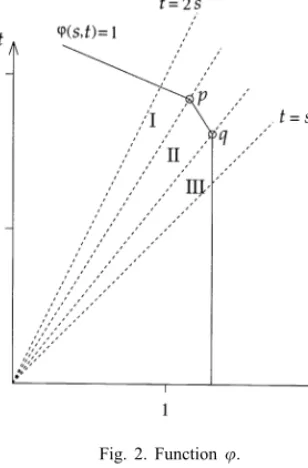
We only consider’on the region of all (s; t) withs6t62sin the positive quadrant. This region is shown in Fig. 2. One can verify that the set of all (s; t) with ’(s; t) = 1 consists of three segments which meet in p= (p1; p2) and q= (q1; q2), as shown in Fig. 2. Therefore, we divide the considered region into three sectors by the lines
t= (p2=p1)sandt= (q2=q1)s. We number the sectors from top to bottom by I, II, and III. Note that ’ is linear within each sector.
We now prove the rst inequality of the lemma. In the following assume thats;s; t;˜ t˜ fulll the condition for the rst inequality. We have to show that(s;s; t;˜ t˜) is nonneg-ative, where :R4
+→Ris dened by
(s;s; t;˜ t˜):=(’(s; t)1=ÿ+’(˜s;t˜)1=ÿ)ÿ−’(s+ ˜s;2s+ ˜t):
Let ’1(s; t) denote the partial derivative of ’(s; t) with respect to s and, accordingly, let’2(s; t) denote the partial derivative with respect to t. is monotonically increasing in ˜s since it is continuous and, on every line in ˜s-direction, @=@s˜is dened on all but at most four points with
@
@s˜(s;s; t;˜ t˜) =ÿ(’(s; t)1=ÿ+’(˜s;t˜)1=ÿ)ÿ−1 1
ÿ’(˜s;t˜)1=ÿ−1’1(˜s;t˜)
Fig. 2. Function’. = 1 + ’(s; t) ’(˜s;t˜) 1=ÿ!ÿ−1 ’1(˜s;t˜)−’1(s+ ˜s;2s+ ˜t) ¿’1(˜s;t˜)−’1(s+ ˜s;2s+ ˜t) ¿0:
The last inequality follows from the fact that, in the positive quadrant, moving in the direction of the vector (1;2) never increases ’1. The function ’1 is constant within each of sectors I, II, and III, with the smallest value in I and the largest value in III. Since the lines bounding the sectors have a slope of at most 2, the last inequality is correct.
Thus, we can choose the least possible value for ˜swhich is ˜s=s by the assumptions for the rst inequality. Furthermore, using ’(cs; ct) =|c|’(s; t) we obtain
(s; s; t;t˜) =s(1;1; t=s;t=s˜ ):
Hence, it is sucient to prove that (1;1; t;t˜)¿0 for arbitrary t; t˜with 16t˜6t62. Now dene ˆ on the triangle D⊆R2
+ with the corners (1;1);(2;1);(2;2) by ˆ
(t;t˜):=(1;1; t;t˜) = (’(1; t)1=ÿ+’(1;t˜)1=ÿ)ÿ−’(2;2 + ˜t):
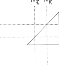
It remains to show that ˆ is nonnegative on D. As shown in Fig. 3, the four linest=
q2=q1; t=p2=p1, ˜t=q2=q1, and ˜t=p2=p1 partitionDinto six regions, which are triangles and rectangles. Restricted to each of these regions, ˆ is a “linear transformation” of the function :R2
+→R+ dened by (x; y):=(x1=ÿ+y1=ÿ)ÿ:
Fig. 3. TriangleD. This means, there are linear functions ‘1; ‘2; ‘3 such that
ˆ
(t;t˜) =‘1(t;t˜) + (‘2(t); ‘3(˜t)):
Note that also’(2;2+˜t) is linear on the intervals [1; q2=q1];[q2=q1; p2=p1] and [p2=p1;2], since 2 +q2=q1= 2p2=p1.
Next we show that is concave onR2. This can be done by proving that the matrix of second-order partial derivatives is negative semi-denite. More explicitly, we have to check that @2 @x2 (x; y)60; @2 @y2 (x; y)60; and @2 @x@y (x; y) 2 − @2 @x2 (x; y) @2 @y2 (x; y) 60:
We omit the tedious but simple calculations. It follows that the function ˆ is concave on each of the six regions of D. Thus the minimum value of ˆ on D appears on a corner of one of the six regions.
It is ˆ(q2=q1; q2=q1) = 0. Again using a symbolic algebra tool, one can verify that ˆ is positive on the other nine corners of the regions. Thus, is non-negative on D and we have proved the rst inequality of the lemma.
The second claim of the lemma is proved analogously. Assume that s;s; t;˜ t˜ fulll the condition of the second claim. Setting
(s;s; t;˜ t˜):=(’(s; t)1=ÿ+’(˜s;t˜)1=ÿ)ÿ−’(s+ ˜t; t+ ˜t); we need to show that (s;s; t;˜ t˜)¿0. Since
@ @t(s;s; t;˜ t˜) = 1 + ’(˜s;t˜) ’(s; t) 1=ÿ!ÿ−1 ’2(s; t)−’2(s+ ˜t; t+ ˜t)
¿’2(s; t)−’2(s+ ˜t; t+ ˜t) ¿0;
is monotonically increasing in t. Again, the last inequality follows from the fact that moving in direction of (1;1) never increases’2. Thus we can restrict ourselves tot=˜t= 1 and s6s˜. Dene ˆon the triangleD0⊆R2
+ with the corners (0:5;0:5); (0:5;1); (1;1) by
ˆ
(s;s˜):=(s;s;˜1;1) = (’(s;1)1=ÿ+’(˜s;1)1=ÿ)ÿ−’(s+ 1;2):
The four lines s=p1=p2; q1=q2; s˜=p1=p2, and q1=q2 divide D0 into six regions. On each of those regions ˆ is a linear transformation of , and thus concave (note that also ’(s+ 1;2) is linear on every region since p1=p2+ 1 = 2q1=q2). Evaluating ˆ on the 10 corners of the regions shows that ˆ(p1=p2; p1=p2)=0; ˆ(0:5;0:5)=0, and ˆ ¿0 on the other corners. This completes the proof of the second claim.
Lemma 12. Letf be a function onn variables representable by a read-once formula. Then we have
’(size(f);size(f;f))6’(1;2)nÿ; where ÿ:=log4(3 +√5)¡1:1943.
Proof. We prove the lemma by induction on n. For n= 1 the claim holds since size(f)61 and size(f;f)62 in this case.
Let n ¿1 and let f be computed by f=g⊗h, where g and h are functions on k
and m variables respectively. Set ˜=’(1;2). By the induction hypothesis we have
’(size(g);size(g;g))6( ˜1=ÿk)ÿ; and
’(size(h);size(h;h))6( ˜1=ÿm)ÿ: We distinguish two cases according to ⊗.
Case 1:⊗=∧. We assume w.l.o.g. that
size(g)¡size(h) or size(g) = size(h) ∧ size(h;h)6size(g;g):
Then Cases 1 and 3 in Section 3 together with the rst inequality of Lemma 11 yield
’(size(f);size(f;f))6’(size(g) + size(h);2 size(g) + size(h;h)) 6( ˜1=ÿk+ ˜1=ÿm)ÿ
= ˜nÿ:
Case 2:⊗=⊕. We assume w.l.o.g. that
Then Cases 2 and 4 in Section 3 together with the second part of Lemma 11 yield
’(size(f);size(f;f))6’(size(g) + size(h;h);size(g;g) + size(h;h)) 6( ˜1=ÿk+ ˜1=ÿm)ÿ
= ˜nÿ:
Theorem 13. Let f be a function on n variables representable by a read-once for-mula. Then size(f)6nÿ and size
ce(f)6nÿ; where :=’(1;2)=’(1;1)¡1:3592.
Proof. By the preceding lemma, ’(size(f);size(f;f))6’(1;2)nÿ. Using the already mentioned facts that ’(1; t) is monotonically increasing in t and that, for s; t; c ∈ R+; ’(cs; ct) =c’(s; t), we have
size(f) =’(size(f);size(f;f))’(1;size(f;f)=size(f))−1 6’(1;2)nÿ’(1;1)−1
=nÿ
with :=’(1;2)=’(1;1)¡1:3592. Analogously, we get
size(f;f) =’(size(f);size(f;f))’(size(f)=size(f;f);1)−1 6’(1;2)nÿ’(0:5;1)−1
= 2nÿ:
Applying Theorem 10, we get sizece(f)6nÿ.
So OBDDs for all read-once formulas are quite small. In order to nd out how tight this bound really is, it is desirable to nd functions representable by read-once formulas which have OBDDs “as large as possible” for a given number of variables.
We restrict ourselves to read-once formulas consisting of ∧- and ⊕-gates only. In general,⊕-gates are more dicult than ∧-gates. Moreover, the proof of the older upper bound of Wegener [27] indicates that we should consider read-once formulas based on balanced trees. We investigate complete binary trees with alternating levels of ∧- and ⊕-gates, where the gate at the root is an⊕-gate. Since x1⊕x2⊕x3⊕x4 is harder than
x1x2⊕x3x4 for OBDDs without complemented edges, we sometimes use only ⊕-gates at the two bottom-most levels above the leaves. This leads to the following function, called Reed–Muller-tree (RMT), since the Reed–Muller decomposition rule is based on ∧- and ⊕-gates.
Deÿnition 14. The function RMTn is represented by a read-once formula which is a complete binary tree with n= 2k variables as leaves and k gate levels numbered from 0 to k−1 starting at the root. The root (level 0) is an ⊕-level. If k is odd, the levels
alternatingly consist of⊕- and∧-gates only. Ifk is even, the levels are also alternating with the exception that level k−1 also consists of ⊕-gates. If n= 1; RMT1(x1) =x1.
Theorem 15. Let n= 2k; wherek is a positive integer. Deÿne r:=3 +√5; s:=3−√5; and 1:=12(7 + 3√5); 2:=12(7−3√5); ˜ 1:=101(15 + 7 √ 5); ˜2:=101(15−7 √ 5):
Then the minimal OBDD size of RMTn fulÿlls size(RMTn) =
(
1rk=2−1+2sk=2−1 if k is even; ˜
1r(k−1)=2+ ˜2s(k−1)=2 if k is odd: Moreover; size(RMTn) = (nÿ) for ÿ= log4(3 +
√ 5).
Proof. Let x1; : : : ; xn be the variables in the read-once formula for RMTn. Because of the symmetry of the circuit, any DFS variable ordering is optimal. W.l.o.g we consider the variable ordering = id. For this ordering, we compute the size of the reduced OBDD for RMTn using the recursive equations from Section 3.
Let n= 2k. Let S
k be the size of the reduced OBDD with variable ordering for RMTn and let Tk be the size of the reduced OBDD for (RMTn;RMTn) and ordering
. We know by case inspection that S1= 3; T1= 4; S2= 7, and T2= 8. Now we consider the levels 0 and 1 of the circuit for RMTn. It holds that
RMTn(u; v; x; y) = (RMTn=4(u)∧RMTn=4(v))⊕(RMTn=4(x)∧RMTn=4(y)); whereu; v; x andyare vectors of (n=4) variables each. We abbreviate this asf=(f1∧
f2)⊕(f3∧f4). Then, by the results of Section 3, size(f) = size(f1∧f2) + size((f3∧f4);(f3∧f4))
= size(f1) + size(f2) + 2·size(f3) + size(f4; f4): Hence, Sk= 4Sk−2+Tk−2. Also by the results of Section 3
size(f;f) = size((f1∧f2);(f1∧f2)) + size((f3∧f4);(f3∧f4)) = 2 size(f1) + size(f2; f2) + 2 size(f3) + size(f4; f4): Hence, Tk= 4Sk−2+ 2Tk−2.
Altogether, we have obtained a system of linear dierence equations for Sk andTk. For the ease of notation, we set U‘:=S2(‘+1); V‘:=T2(‘+1) if k = 2(‘+ 1); ‘¿0 (k even) and U‘:=S2‘+1; V‘:=T2‘+1 if k= 2‘+ 1; ‘¿0 (k odd) and consider the system
U‘ V‘ = 4 1 4 2 U‘−1 V‘−1 ; ‘¿1:
Let A be the coecient matrix of this system. An exact solution can be obtained by standard methods, e.g., by the general method based on generating functions described
in [11]. Since we have a simple homogeneous system, we prefer to apply the analogue of the well-known method for solving lineardierentialequations with constant coe-cients (cf. [15, chapter 6]). This method is based on the computation of the eigenvalues and eigenvectors of the coecient matrix A. Here, the general solution of the system is of the form U‘ V‘ =1b1r‘+2b2s‘; ‘¿0;
where 1; 2 ∈R are arbitrary coecients, r and s as dened in the theorem are the eigenvalues of A (each with multiplicity 1) and b1 and b2, resp., are corresponding eigenvectors, e.g.,
b1= (1;−1 +√5)> and b2= (1;−1−√5)>:
The coecients 1 and2 are determined by the initial values. For even k, we have
u0 V0 = S2 T2 = 7 8 = 1 1 −1 +√5; −1−√5 1 2
with the solution 1= (1=2)(7 + 3√5) and 2= (1=2)(7−3√5). For odd k,
u10 V0 = S1 T1 = 3 4 = 1 1 −1 +√5; −1−√5 ˜ 1 ˜ 2
with the solution ˜1= (1=10)(15 + 7√5) and ˜2= (1=10)(15−7√5).
We remark that we have also obtained an exact formula for Tk as a “by-product”:
Tk= ( 1(−1 + √ 5)rk=2−1+ 2(−1− √ 5)sk=2−1 if k is even; ˜ 1(−1 + √ 5)r(k−1)=2+ ˜ 2(−1− √ 5)s(k−1)=2 if k is odd:
This is interesting since Tk=2 is the size of the optimal OBDD with complemented edges for RMTn and n= 2k. The lower bound for the OBDD size of RMTn matches asymptotically with the upper bound from Theorem 13. For the innitely manyn where
k is odd, the constant factor of nÿ is ˜
1r−1=2¿1:3395 by Theorem 15. To see how close the bounds are for some n, we compare the results in Table 1.
7. Conclusion
The variable ordering problem is crucial for the successful application of OBDDs. In order to better understand the variable ordering problem, we have analyzed the restricted class of functions representable by read-once formulas. We have presented an ecient algorithm for this restricted version of the variable ordering problem, based on an extensive analysis of the structure and size of optimal OBDDs. Furthermore, we have proved that the size of optimal OBDDs for functions which are representable by read-once formulas cannot become large. On the other hand, there are functions with read-once formulas which are not representable by OBDDs of linear size.
Table 1
Upper and lower bounds
OBDDs OBDDs with compl. edges
Old upper bound New upper bound Lower bound Upper bound Lower bound
n nlog 3 nÿ size(RMTn) nÿ sizece(RMTn)
32 243 85 84 62 52 64 729 195 188 143 116 128 2187 446 440 328 272 256 6561 1021 984 751 608 512 19,683 2337 2304 1719 1424 1024 59,049 5349 5152 3935 3184 Acknowledgements
We would like to thank the anonymous referee for helpful comments and suggestions.
References
[1] D. Angluin, L. Hellerstein, M. Karpinski, Learning read-once formulas with queries, J. ACM 40 (1993) 185–210.
[2] B. Bollig, M. Lobbing, I. Wegener, Simulated annealing to improve variable orderings for OBDDs. International Workshop on Logic Synthesis (IWLS), 5/1–5/10, May 1995.
[3] B. Bollig, I. Wegener, Improving the variable ordering of OBDDs is NP-complete, IEEE Trans. Comput. 45 (9) (1996) 993–1002.
[4] R.E. Bryant, Graph-based algorithms for Boolean function manipulation, IEEE Trans. Comput. C-35 (8) (1986) 677–691.
[5] R.E. Bryant, Symbolic Boolean manipulation with ordered binary-decision diagrams, ACM Comput. Surveys 24 (3) (1992) 293–318.
[6] N.H. Bshouty, T.R. Hancock, L. Hellerstein, Learning Boolean read-once formulas over generalized bases, J. Comput. System Sci. 50 (1995) 521–542.
[7] K.M. Butler, D.E. Ross, R. Kapur, M.R. Mercer, Heuristics to compute variable orderings for ecient manipulation of ordered binary decision diagrams, Proceedings of the 28th ACM/IEEE Design Automation Conference (DAC), 1991, pp. 417–420.
[8] H. Fujii, G. Ootomo, C. Hori, Interleaving based variable ordering methods for ordered binary decision diagrams, Proceedings of the ACM/IEEE International Conference on Computer Aided Design (ICCAD), 1993, pp. 38–41.
[9] M. Fujita, H. Fujisawa, N. Kawato, Evaluation and improvements of Boolean comparison method based on binary decision diagrams, Proceedings of the ACM/IEEE International Conference on Computer Aided Design (ICCAD), 2–5, November 1988.
[10] M. Fujita, Y. Matsunaga, T. Kakuda, On variable ordering of binary decision diagrams for the application of multi-level logic synthesis, Proceedings of the European Design Automation Conference (EDAC), 1991, pp. 50–54.
[11] R.L. Graham, D.E. Knuth, O. Patashnik, Concrete Mathematics, Addison-Wesley, Reading, MA, 1994. [12] G.D. Hachtel, F. Somenzi, A symbolic algorithm for maximum ow in 0–1-networks, Formal Methods
System Des. 10 (1997) 207–219.
[13] R. Heiman, I. Newman, A. Wigderson, On read-once threshold formulae and their randomized decision tree complexity, Theoret. Comput. Sci. 107 (1993) 63–76.
[14] N. Ishiura, H. Sawada, S. Yajima, Minimization of binary decision diagrams based on exchange of variables, Proceedings of the ACM/IEEE International Conference on Computer Aided Design (ICCAD), 1991, pp. 472–475.
[15] R. Lidl, H. Niederreiter, Introduction to Finite Fields and Their Applications, Cambridge University Press, Cambridge, 1994.
[16] M. Lobbing, I. Wegener, The number of knight’s tours equals 33,439,123,484,294 — counting with binary decision diagrams, Electron. J. Combin. 3(#R5) (1996) 1–4.
[17] S. Malik, A.R. Wang, R.K. Brayton, A.L. Sangiovanni-Vincentelli, Logic verication using binary decision diagrams in a logic synthesis environment, Proceedings of the ACM/IEEE International Conference on Computer Aided Design (ICCAD), 6–9, November 1988.
[18] M.R. Mercer, R. Kapur, D.E. Ross, Functional approaches to generating orderings for ecient symbolic representations, Proceedings of the 29th ACM/IEEE Design Automation Conference (DAC), 1992, pp. 624–627.
[19] S. Minato, N. Ishiura, S. Yajima, Shared binary decision diagram with attributed edges for ecient Boolean function manipulation, Proceedigns of the 27th ACM/IEEE Design Automation Conference (DAC), June 1990, pp. 52–57.
[20] S. Panda, F. Somenzi, Who are the variables in your neighborhood, International Workshop on Logic Synthesis (IWLS), 5/11–5/20, May 1995.
[21] R.L. Rudell, Dynamic variable ordering for ordered binary decision diagrams, Proceedings of the ACM/IEEE International Conference on Computer Aided Design (ICCAD), November 1993, pp. 42– 47.
[22] D. Sieling, The nonapproximability of OBDD minimization, Technical Report 663, Universitat Dortmund (1998) Submitted to Information and Comput.
[23] D. Sieling, On the existence of polynomial time approximation schemes for OBDD minimization, Proceedings of the 15th Annual Symposium on Theoretical Aspects of Computer Science (STACS), Lecture Notes in Computer Science, Vol. 1353, Springer, Berlin, 1998.
[24] D. Sieling, I. Wegener, NC-algorithms for operations on binary decision diagrams, Parallel Process. Lett. 3 (1) (1993) 3–12.
[25] D. Sieling, I. Wegener, On the representation of partially symmetric Boolean functions by ordered multiple valued decision diagrams, Multiple Valued Logic 4 (1998) 63–96.
[26] I. Wegener, Optimal decision trees and one-time-only branching programs for symmetric Boolean functions, Inform. and Control 62 (2/3) (1984) 129–143.
[27] I. Wegener, Comments on A characterization of binary decision diagrams, IEEE Trans. Comput. 43 (1994) 383–384.
[28] I. Wegener, Branching Programs and Binary Decision Diagrams — Theory and Applications, Monographs on Discrete and Applied Mathematics, SIAM, Philadelphia, PA, to appear.