°
W
HAT
D
O
W
E
D
O WITH
M
ISSING
D
ATA
? S
OME
O
PTIONS FOR
A
NALYSIS OF
I
NCOMPLETE
D
ATA
Trivellore E. Raghunathan
Department of Biostatistics and Institute for Social Research,
University of Michigan, Ann Arbor, Michigan 48109; email: [email protected]
■ Abstract Missing data are a pervasive problem in many public health investiga-tions. The standard approach is to restrict the analysis to subjects with complete data on the variables involved in the analysis. Estimates from such analysis can be biased, especially if the subjects who are included in the analysis are systematically different from those who were excluded in terms of one or more key variables. Severity of bias in the estimates is illustrated through a simulation study in a logistic regression setting. This article reviews three approaches for analyzing incomplete data. The first approach involves weighting subjects who are included in the analysis to compensate for those who were excluded because of missing values. The second approach is based on multiple imputation where missing values are replaced by two or more plausible values. The final approach is based on constructing the likelihood based on the incom-plete observed data. The same logistic regression example is used to illustrate the basic concepts and methodology. Some software packages for analyzing incomplete data are described.
Key Words available-case analysis, observed data likelihood, missing data mechanism, multiple imputation, nonresponse bias, weighting
INTRODUCTION
Missing data are a ubiquitous problem in public health investigations involving human populations. In a cross-sectional study relying on a survey, subjects may refuse to participate entirely or may not answer all the questions in the question-naire. The former type of missing data is called unit nonresponse, and the latter, item nonresponse. In a longitudinal study, subjects may drop out, be unable, or refuse to participate in subsequent waves of data collection. The missing data in this context may be viewed as unit or item nonresponse. For instance, in a cross-sectional analysis of data from a particular wave, drop-outs may be viewed as unit nonrespondents, whereas in a longitudinal analysis involving data from all waves, missing data due to drop-outs may be viewed as item nonresponse.
The standard approach, a default option in many statistical packages, is to restrict the analysis to subjects with no missing values in the specific set of variables. This
so-called available-case analysis can yield biased estimates. Sometimes, where multiple analyses are involved, including descriptive analysis, the standard ap-proach excludes subjects with any missing values in any of the variables used in at least one analysis (the so-called complete-case or listwise deletion analysis). Other ad hoc approaches such as treating the missing data as a separate category also result in biased estimates (35).
To demonstrate the potential bias in the available-case estimates, consider a population with a binary disease variable, D, a binary exposure variable, E, and a continuous confounder, x. Suppose that this population adheres to the following model assumptions:
x∼N (0,1),
logit Pr(E=1|x)=0.25+0.75×x,and
logit Pr(D=1|x,E)= −0.5+0.5×E+0.5×x.
This model and the parameters were partly motivated by the analysis of cohort data. A sample size of 1000 is drawn from essentially an infinite population, and a logistic regression model is fitted, with D as the outcome variable and x and E as predictors (the last equation in the above model assumptions), resulting in the estimates of −0.54, 0.57, and 0.53 for the intercept, regression coefficients for
E and x, respectively. These estimates are close to the true values in the logistic
regression model given above.
Now suppose that some values of x are deliberately set to be missing using the following logistic model,
logit[Pr(x is missing)]= −1.11−1.09×D−1.85×E+2.31×D×E.
That is, for each subject, generate a uniform random number between 0 and 1, and if this number is less than or equal to the probability computed from the above equation, then set that value of x to missing. This model for deleting values was designed to produce approximately 15% missing values, and the percentage of observations with missing values in the 4 cells formed by D and E was 26% for (D =0, E =0), 11% for (D =1, E= 0), 5% for (D =0, E =1), and 14% for (D = 0, E = 0). These parameters were chosen to match the missing values in the cohort data that motivated this experiment. The same logistic regression model was fitted to the data set, now restricted only to those subjects with no missing values in x. The resulting estimates of intercept, regression coefficients for E and x were−0.30, 0.28, and 0.52, respectively. The estimate of the regression coefficient for E is remarkably different when compared to the “before-deletion” estimate as well as the true value of 0.5. One might wonder whether the observed difference is due to idiosyncrasies of this particular data set or has occurred purely by chance.
To investigate further, the experiment was replicated as follows:
1. Generate 2500 samples (we will call these before-deletion samples) each of size 1000.
2. Delete some values of x in each data set using the same logistic model mechanism given above (we will call the corresponding data sets with values of x set to missing as “after-deletion” data sets).
3. Fit logistic regression models to both 2500 before-deletion and the corre-sponding after-deletion data sets.
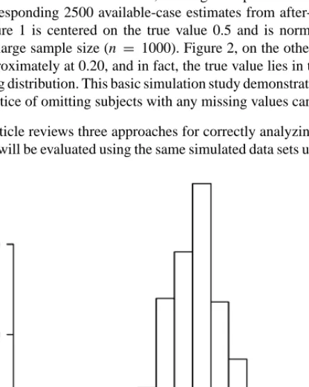
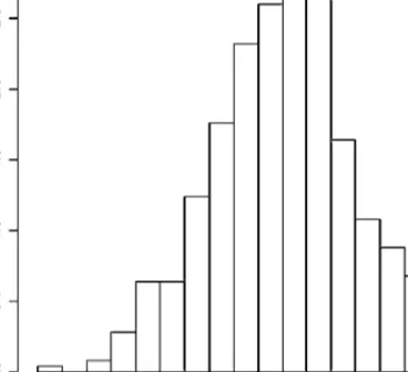
4. The primary parameter of interest is the regression coefficient for E, the log-odds ratio measuring the association between D and E adjusted for x. Figure 1 provides the histogram of 2500 estimated regression coefficients from before-deletion data sets, and Figure 2 provides the histogram of the corresponding 2500 available-case estimates from after-deletion data sets. Figure 1 is centered on the true value 0.5 and is normal in shape, given the large sample size (n = 1000). Figure 2, on the other hand, is centered approximately at 0.20, and in fact, the true value lies in the tail of the sam-pling distribution. This basic simulation study demonstrates that the standard practice of omitting subjects with any missing values can be invalid. This article reviews three approaches for correctly analyzing incomplete data, and these will be evaluated using the same simulated data sets used to illustrate the
Figure 1 Histogram of logistic regression coefficient from 2500 simulated data sets before deleting any covariate values.
Figure 2 Histogram of logistic regression coefficient from 2500 simulated data sets after deleting some covariate values and using available-cases.
perils of using the available-case approach. The first approach involves attaching weights to each subject included in the analysis to represent subjects who were excluded. This is often used to compensate for unit nonresponse in surveys [see (9) for a review]. The second approach is through multiple imputation (29, 30), where the missing set of values is replaced by more than one plausible set of values. Each plausible set of values in conjunction with the observed data results in a completed data set. Each completed data set is analyzed separately using the standard complete data software, and the resulting point estimates and standard errors are combined using a simple formula described later.
The distinction between the observed and filled-in values must be incorpo-rated in any subsequent analysis of data with imputed values. That is, the filled-in values for any one subject with missing values should not be considered as micro-data for that subject but rather as values that are statistically plausible given other information on that subject. These filled-in or completed data sets are plausible samples from the population under certain assumptions. Thus, the completed data sets should result in inferences (point estimates and confidence intervals, for ex-ample) that are within the realm of statistical plausibility of inferences that would have been obtained had there been no missing data. In that respect, the multiple imputation approach is a statistical approach of “rectangularizing” the observed
data to exploit the available complete data software to obtain valid inferences. The inferential validity based on the multiple imputed data sets is the goal, and any imputation procedure should not viewed as a method for recovering the missing values for any given individual.
The third approach is based on the likelihood constructed from the observed in-complete data. This approach has a long history: The earliest reference seems to be McKendrick (21), who used an algorithm similar to the Expectation-Maximization (EM) algorithm (5) to obtain estimates from a sample with missing values. The EM algorithm is a popular approach for maximizing the observed data likelihood. This paper emphasizes weighting and imputation approaches and briefly discusses the maximum likelihood approach. The maximum likelihood approach is available only for very few selected models such as multivariate normal linear regression, contingency tables, and certain other multivariate analyses. A detailed discussion of the maximum likelihood approach can be found in Reference 19 and a Bayesian approach similar in spirit in Reference 34.
All these methods make certain assumptions about why data are missing. The answer to this question is stated in terms of assumptions about the missing data mechanism. In the next section, this critical concept is described. The missing data mechanisms comprise probabilistic specifications of why data are missing. These mechanisms were developed by Rubin (28) and later extended to longitu-dinal data by Little (17). All three approaches described above are valid under the so-called missing at random (MAR) mechanism, and, generally, the available-case approach is valid under a stricter mechanism called missing completely at random (MCAR). The third section describes the weighting approach; the fourth section, the multiple imputation approach; and the fifth section describes the likelihood-based methods. The final section concludes with discussion and limitations.
MISSING DATA MECHANISM
To understand the taxonomy of missing data mechanisms, consider a simple case where the analysis of interest is concerned with a set of variables (U, V), the missing values are in a single variable U, and variables in vector V have no missing values. Our simulation study falls into this category. Suppose that R denotes an indicator variable taking the value 1 if U is observed and 0 if U is not observed. Thus, the observed data are R, (U, V), if R =1 and V, if R = 0. The missing data mechanism or, equivalently, the response mechanism is the conditional probability distribution of R, Pr(R|U,V), given (U, V). That is, what probabilistic mechanism
governs the observation of U, specifically in relation to the variables of interest U and V?
The missing data mechanism is called MCAR, if Pr(R = 1|U,V) = c, a
con-stant. That is, the probability that U is observed is independent on the underlying values of U or V. Under this assumption, the available-cases (that is, with R = 1) constitute a random subsample of the original sample. In a more general case,
where missing values can also occur in V, the MCAR assumption implies that the missing values in any variable are independent of the underlying values of U or V. The subjects included in the available-case analysis, therefore, constitute a random subsample of the original sample. Thus, the analysis that includes only those who have U and V observed is generally valid under this assumption because the process of excluding the subjects with any missing values does not distort the representativeness of the original sample. This assumption is clearly violated in our simulation study where the percentages with missing values differ across the four cells based on D and E. The MCAR is a rather strong assumption and is rarely satisfied in practical applications. Sometimes the available-case analysis may be valid under a weaker assumption [see, for example, (7, 12, 15)], but these exceptions are few and idiosyncratic.
A weaker assumption is MAR where, again, resorting to the simple case first,
Pr(R = 1|U,V) = f(V), a function that depends on V but not on U. The
dele-tion mechanism used in the simuladele-tion study falls under this category where the missingness in x depends on D and E but not on x. In essence, this assumption entails that for two individuals with the same value of V, one has U observed and the other has U missing; the missing U is arising from the same distribution (for a given V) as the observed one. That is, conditional on V, the missing U is predictable from the observed distribution of U. In a more general situation where the missing values can be in several variables, the exact analytical specification of this assumption is difficult. Loosely speaking, suppose that di,obs denotes the observed components of complete data, (Ui,Vi), for subject i, and di,mi ssdenotes the missing components. For two individuals, i and j, when di,obs = dj,obs, the missing components, di,mi ss and dj,mi ss, have the same distribution.
Given this conditional nature of the assumption, the stronger the correlates of
U in V, the weaker is the assumption about the missing data mechanism for U.
For example, if U were income, then having a rich set of variables to condition on in V, such as age, gender, education, occupation, property values, monthly expenditures, and neighborhood level information, makes the assumption about missing data considerably weaker when compared to MCAR or when the list of variables to be conditioned on is limited to, say, age and gender. The limitation of the MAR assumption is due to lack of appropriate variables that can be con-ditioned on in the analysis, and empirically it has been shown to be reasonable in practical situations (4, 33). The three approaches discussed in this paper are valid under different versions of this weaker assumption about the missing data mechanism.
Finally, the missing data mechanism is said to be Not-Missing at Random (NMAR), if Pr(R= 1|U, V)= f(U, V), a function that certainly depends on U but
may also depend on V. That is, even after conditioning on V, the distribution of U for the respondents and nonrespondents are dissimilar. This function, however, is not estimable from the observed data because whenever R =0, U is unobserved.
Therefore, an explicit form of f has to be specified and the data cannot be used to empirically verify the validity of this assumption.
The specification of Pr(R=1|U, V), in conjunction with the substantive model Pr(U, V), is used to construct inferences about the parameters of interest. This is
a selection model method and was first proposed by Heckman (8). The alternative approach is to specify how different the distributions of (U, V) are for the respon-dents and nonresponrespon-dents. That is, specify the population distribution as a mixture of two components, Pr(U, V|R=1) and Pr(U, V|R=0), for respondents and non-respondents, respectively. This mixture is used to construct inferences about the population. Again, there is no data to specify the part of the mixture Pr(U, V|R =
0) because U is unobserved whenever R =0. This approach was first proposed by Rubin (27, 29) and later extended by Little (16). In any event, both these approaches make empirically unverifiable assumptions, and their use is very limited to situ-ations where some prior knowledge may exist to specify the mixture distribution or the selection model. For more details see Chapter 15 in Reference 19.
WEIGHTING
The origins of weighting may be traced to sample survey practice where it is used as a simple device to account for unequal probabilities of selection (11). The survey weight for an individual is the inverse of his/her selection probability. To be concrete, suppose that a national probability survey sampled 1000 subjects with 500 Whites and 500 African Americans. That is, the African Americans were oversampled with respect to their representation in the population. Suppose that one were to ignore this fact and proceeded to compute a simple average of 1000 observations as an estimate of the population mean. If there are large differences between Whites and African Americans in the survey variable of interest, the sample mean will be a distorted representation of the population mean. Down-weighting the observations on African Americans to their representation in the population and up-weighting the observations on Whites to their representation in the population would obtain the accurate picture of the population. Thus, the weighted average (where the weights are inverse of their selection rate) is an unbiased estimate of the population mean whereas the simple mean is not. However, special software is needed to compute standard errors and confidence intervals that use these weights. Currently, popular packages such as SAS, STATA, and SUDAAN have built-in routines to take into account these survey weights.
Weighting to compensate for nonresponse is an extension of the same idea. That is, excluding the subjects because of missing values is a distortion of the representation in the original sample, and weights are attached to subjects included in the analysis to restore the representation. To be concrete, consider the simulation example. Suppose that ndeis the number of subjects with D =d and E=e where
d, e = 0,1. Let the number of subjects with observed x in the corresponding cell be rde. To restore the available-case analysis to its original sample representation, we should weight each respondent in (d, e) cell bywde=nde/rde, inverse of the response rate in that cell or the inverse of the selection probability into the data
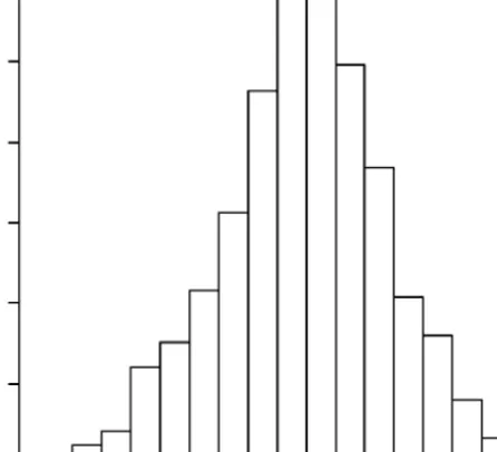
Figure 3 Histogram of logistic regression coefficient from 2500 simulated data sets after deleting some covariate values and using weights to compensate for missing data.
analysis. A weighted logistic regression can be used to estimate the parameter of interest (2).
Figure 3 gives the point estimates for the same 2500 data sets analyzed previ-ously, but this time based on weighted logistic regression where the weights were computed as the inverse of the response rates in the four cells. As can be seen, the weighted estimates are unbiased and, understandably, slightly more variable than the before-deletion estimates.
There are several approaches for constructing weights (9). Consider the example given earlier where the analysis of interest is concerned with a set of variables (U,
V), the missing values are in a single variable U, and variables in a vector V have no
missing values. The adjustment-cell method involves constructing a contingency table through cross-classification of sampled subjects based on V. The inverse of the response rate in any cell is the weight attached to each respondent in that cell. The underlying assumption is that, conditional on belonging to an adjustment cell, the respondents and nonrespondents have similar distribution of variables with missing values (that is, respondents and nonrespondents are exchangeable within
the adjustment cell). The simulation example described above used this method to construct the weights based on D and E. The disadvantage of this approach is that the continuous variables in V have to be categorized, and if V has a large number of variables, the contingency table can be sparse, leading to unstable weights.
An alternative approach is to estimate the response propensity through a logistic regression model, Pr(R =1|V )=[1+exp(−βo−Vtβ1)]−1, whereβo andβ1are the unknown regression coefficients and the superscript t denotes matrix transpose. Suppose that ˆβo and ˆβ1are the estimated regression coefficients; the weights for a respondent j is then defined aswj =1+exp(−βˆo−Vjtβˆ1). One may include the interaction terms between different variables or transformation in V. There is no need to categorize continuous variables. This response propensity approach is more practical when we have large numbers of variables. Sometimes categorization of estimated response probabilities forms adjustment cells.
MULTIPLE IMPUTATION
Weighting is a simple approach for making the subjects included in the available-case analysis representative of the original sample and is effective in removing nonresponse bias. However, by including only subjects with complete data, it ignores partial information from subjects with incomplete data. For example, in a multiple linear regression with some subjects missing one variable at the most, it can be very inefficient to ignore information on the rest of the variables, especially if they are good predictors of the variables with missing values.
An alternative approach is based on filling in or imputing the missing values in the data set. Again, this approach can be traced back to survey practices adopted by the U.S. Bureau of Census [See (6) for historical accounts]. This practice of filling in the missing values (this is called single imputation method) in the survey practice is attractive for several reasons. First, imputation adjusts for differences between nonrespondents and respondents on variables observed for both and in-cluded in the imputation process, as well as differences on variables not inin-cluded in the model that are predicted by the model; such an adjustment is generally not made by available-case analysis. Second, the complete data software can be used to process the data to obtain descriptive statistics and other statistical measures. This is a significant advantage because complete-data software has kept closer pace with the statistical methodological developments than the incomplete-data software. Third, when a data set is being produced for analysis by the public or multiple researchers, imputation by the data producer allows the incorporation of specialized knowledge about the reasons for missing data in the imputation pro-cedure, including confidential information that cannot be released to the public or other variables in the imputation process that may not be used in substantive anal-ysis by a particular researcher. Raghunathan & Siscovick (24) demonstrate that using an auxiliary variable in the imputation process can improve the efficiency considerably. Moreover, the nonresponse problem is solved in the same way for
all users so that analyses will be consistent across users. The researcher using the filled-in data can concentrate on addressing substantive questions of interest and not be distracted by incomplete data. See Reference 31 for a detailed list of applications of this approach.
Although single imputation, that is, imputing one value for each missing datum, enjoys the positive attributes just mentioned, analysis of a singly imputed data set using standard software fails to reflect the uncertainty due to the fact that the imputed values are plausible replacements for the missing values but are not the true values themselves. As a result, such analyses of singly imputed data tend to produce estimated standard errors that are too small, confidence intervals that are too narrow, and significance tests with p-values that are too small.
Multiple imputation (29, 30) is a technique that seeks to retain the advantages of single imputation while also allowing the uncertainty due to imputation to be incorporated into the analysis. The idea is to create more than one, say M, plausible sets of replacements for the missing values, thereby generating M completed data sets. The variation across the M completed data sets reflects the uncertainty due to imputation. Typically, M is not larger than five.
The analysis of the M completed data sets resulting from multiple imputation proceeds as follows:
1. Analyze each completed data set separately using a suitable software package designed for complete data (for example, SAS, SPSS, or STATA).
2. Extract the point estimate and the estimated standard error from each analysis.
3. Combine the point estimates and the estimated standard errors to arrive at a single point estimate, its estimated standard error, and the associated confidence interval or significance test.
Suppose elis the estimate and slits standard error, based on the completed data set l =1,2,· · ·,M, whereM≥2. The multiply imputed estimate is the average,
¯eM I = 1 M M X l=1 el,
and the standard error of the multiply imputed estimate is
sM I = r ¯uM+ M+1 M bM, where ¯uM = 1 M M X l=1 sl2 and
bM = 1 M−1 M X l=1 ¡ el−¯eM I ¢2
The sampling variance (term inside the square root sign) has two parts: The first part is the average sampling variance by treating the imputed values as though they are real. This is called within-imputation component of variance. The second part is the variability across the imputed values (the between-imputation component of variance), which is not estimable unless more than one plausible set of values are used as fill-in. Rubin & Schenker (32) and Rubin (30) derived the sampling distribution as t-distribution with degrees of freedom,ν = (M −1)(1+rM)2, where rM = ¯uM/[(1+M−1)bM]. Several other methods have been developed to construct intervals (1, 13, 14).
Most straightforward justification for generating more than one plausible set of values is through draws from the predictive distribution of the missing val-ues conditional on the observed valval-ues. Revisiting the simulation example, one could generate several plausible values from the predictive distribution based on a regression model,
x=βo+β1D+β2E+β3D×E+ε,
whereβ =(βo, β1, β2, β3) is a vector of regression coefficients, and the residual
ε ∼ N (0, σ2). A simple approach is to estimate the regression coefficients and the residual variance using subjects with x, D, and E observed. Suppose ˆx is the predicted value for an individual with missing x. Adding different noise variables
z∼N (0,σˆ2), where ˆσ2is the estimate of residual variance, to the predicted value generates plausible values. This method is reasonable for large sample size but still is not proper (30) because plausible values are generated without reflecting uncertainty in the estimates of the regression coefficients and residual variances. A proper approach reflects uncertainty in every estimate while generating plausi-ble values. A proper approach for generating the plausiplausi-ble values is the Bayesian approach where the missing values are drawn from the posterior predictive distri-bution of the missing observations conditional on the observed data. The approach is technical and the procedure for the simulation example is described in the ap-pendix. More formal description of a proper method can be found in References 19, 30, and 34.
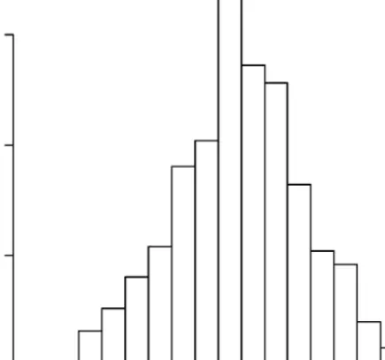
The fully Bayesian approach described in the appendix was implemented on 2500 simulated data sets with missing values described earlier. Five imputations were created for each of 2500 data sets with missing values. Five completed data sets were analyzed by fitting a logistic regression model to each. The multiple imputation estimate and its standard error were computed using the formula given above. Figure 4 gives the histogram of 2500 multiple imputation estimates, which shows that the sampling distribution is centered on the true value 0.5.
The most straightforward approach for creating multiple imputations is model-based using a Bayesian formulation. That is, draw values from the posterior
Figure 4 Histogram of logistic regression coefficient from 2500 simulated data sets after deleting some covariate values and using multiple imputation method.
predictive distribution, Pr(dmi ss|dobs), of the missing values, dmi ss, conditional on the observed values, dobs. Little & Raghunathan (18) argue that the impu-tation should condition on as much observed information as possible to make MAR plausible and imputations efficient. Schafer (34) has developed several rou-tines for implementing the Bayesian method where one can achieve approximate normality of continuous variables through transformation and a limited number of categorical variables (see the website http://www.stat.psu.edu/∼jls). However, this model-building task can be quite difficult in practical situations with hundreds of variables, skip patterns in the questionnaire, different types of variables such as continuous, categorical, count, and semicontinuous (basically, continuous but with a spike at 0). Other common problems include structural dependencies. For example, the question asking about years of smoking is applicable only to current and former smokers, whereas years since quitting is applicable only to former smokers. Also, years smoked cannot exceed the age of the person.
An alternative, though not a fully model-based Bayesian but fully conditional approach, is the sequential regression approach (23), which builds on a version for
continuous variables originally proposed by Kennickel (10). A brief description of SRMI is as follows: Let X denote the fully observed variables, and let Y1,Y2, . . . ,Yk denote k variables with missing values in any order. The imputation process for
Y1,Y2, . . . ,Yk proceeds in c rounds. In the first round, Y1is regressed on X, and the missing values of Y1are imputed (using a process analogous to that described for the logistic regression example in the Appendix); then Y2is regressed on X and
Y1(including the imputed values of Y1), and the missing values of Y2are imputed; then Y3is regressed on X,Y1 and Y2, and the missing values of Y3 are imputed; and so on, until Yk is regressed on X,Y1,Y2. . . ,Yk−1, and the missing values of
Ykare imputed.
In Rounds 2 through c, the imputation process carried out in Round 1 is repeated, except that now, in each regression, all variables except for the variable to be im-puted are included as predictors. Thus, Y1is regressed on (X,Y2,Y3, . . . ,Yk), and the missing values of Y1are imputed; then Y2is regressed on (X,Y1,Y3, . . . ,Yk), and the missing values of Y2 are imputed; and so on. After c rounds, the final imputations of the missing values in (Y1,Y2, . . . ,Yk) are used.
An SAS-based software IVEware implementing this approach is available from the website http://www.isr.umich.edu/src/smp/ive. The S-plus version of a similar approach is available from http://www.multiple-imputation.com. For the regres-sions in the SRMI procedure, IVEware allows the following models:
1. a normal linear regression model if the Y-variable is continuous; 2. a logistic regression model if the Y-variable is binary;
3. a polytomous or generalized logit regression model if the Y-variable is cat-egorical with more than two categories;
4. a Poisson loglinear model if the Y-variable is a count;
5. a two-stage model if the Y-variable is mixed (i.e., semicontinuous). In the first stage zero/nonzero status is imputed using a logistic regression model. Conditional on being nonzero, a normal linear regression model is used to imput a nonzero value.
Because SRMI requires only the specification of individual regression models for each of the Y-variables, it does not necessarily imply a joint model for all of the
Y-variables conditional on X. This procedure compares well with the fully Bayesian
approach as demonstrated through the simulation study by Raghunathan et al. (23). This is the most practical approach in many situations involving structural dependencies and the large number of predictors of varying types.
MAXIMUM LIKELIHOOD
In the complete data statistical methodology, maximum likelihood for a given model is a dominant inferential procedure, for example, the linear, logistic, Poisson, log-linear, and random effects models. All use likelihood as a basis for constructing
inferences. Extending the same notion, one possibility is to base our inferences on likelihood function constructed from the actual observed data set. To motivate this approach, consider an example based on a random sample of size n from a bivariate normal distribution,
µX Y ¶ ∼N ·µµ X µY ¶ , µσ2 X σX Y σX Y σY2 ¶¸ .
Suppose that p subjects provide both X and Y, q subjects provide only X and not Y, and r subjects provide Y but not X. The objective is to estimate the five unknown parameters (µX, µY, σX2, σ
2
Y, σX Y). Once these estimates are obtained, any function of these parameters, such as correlation coefficient or regression coefficients, can be computed. Wilks (36) addressed this estimation problem using several approaches including the maximum likelihood method.
The observed data likelihood is a product of three components,
Lobs=Lp×Lq×Lr,
where the first component is the contribution from p subjects who provided both
X and Y. This is a product of bivariate normal density function evaluated at the
observed values for those p subjects, and it involves all five parameters. The second component is the contribution from q subjects who provided only X. This is a product of univariate normal density functions involving only (µX, σX2). Finally, the third component, based on r subjects who provided only Y, is a product of univariate normal density functions involving only (µY, σY2). The observed data likelihood is then maximized with respect to (µX, µY, σX2, σ
2
Y, σX Y) using some iterative routines such as Newton-Raphson method or, more popular, the EM algorithm (5). More generally, suppose that Yiis a complete data vector on subject i = 1, 2,
. . ., n; Yi,obsdenotes the observed components and Yi,missthe missing components; andYi =(Yi,obs,Yi,mi ss). Suppose the complete data model is
f (Yi|θ)= f (Yi,obs,Yi,mi ss|θ),
whereθis the unknown parameter to be estimated. The observed data likelihood is Lobs(θ)= n Y i=1 L(θ|Yi,obs)∝ n Y i=1 Z f (Yi,obs,Yi,mi ss|θ) dYi,mi ss.
The justification that this is the correct likelihood to be maximized when data are MAR is given in Reference 28.
The approximate sampling variances are typically estimated by inverting the negative second derivative of the logarithm of the observed data likelihood. Though the estimates based on this approach are perhaps the most efficient and enjoy all the nice properties accorded to maximum likelihood estimates, implementa-tion is quite difficult even in the simple logistic regression case considered ear-lier. Typically special software needs to be developed for a particular problem.
Software for multivariate normal model is available in SPSS 10 and as an add-on package in GAUSS. The general location model, which can be used to model normal continuous and discrete variables simultaneously, was considered by Little & Schluchter (20), Raghunathan & Grizzle (22) and Schafer (34). Software for fitting such models using a Bayesian approach was developed by Schafer (34). Due to these technical difficulties, this method is not practical in many real world applications.
DISCUSSION AND LIMITATIONS
Analysis of data with some missing values is an important problem, and the stan-dard strategy of including only those on whom a particular analysis can be carried out can lead to biased estimates. Three approaches have been discussed with in-creasing levels of statistical sophistication. Weighting is the simplest approach; multiple imputation is at the second level but is still a more general approach. The maximum likelihood approach is the most difficult, often requiring user-developed software for implementation. All these approaches are valid under a general class of mechanisms called MAR, whereas the available-case analysis is generally valid under MCAR, though there are some exceptions (7, 12). These exceptions are few and idiosyncratic, and are often difficult to verify in a practical setting. Even if the data are MCAR, the available-case method is less efficient owing to discard-ing subjects with partial information. It is not uncommon for substantial numbers of subjects to be excluded in a regression analysis, even though each subject is missing only a few variables.
Weighting is a simple device to correct for bias, but it suffers from the same disadvantages as the available-case method in terms of efficiency. It still discards partial information from subjects with missing values. Thus, if the bias correction is the motivating factor, then weighting should be used to compensate for missing data. Either the adjustment-cell method or the response propensity method can be used to derive the weights, though the response propensity method relies on the logistic regression model. A compromise might be to use the response propensities to form adjustment cells to rely less on the correctness of the response propensity model specification.
Perhaps the most practical approach is based on multiple imputation. This ap-proach involves an upfront investment in multiply imputing the missing values in the database. Once multiply imputed, any complete data software can be used to repeatedly analyze the completed data sets, extract the point estimates and their standard errors, and combine them using the formula given in the third section of this review. The last step can be carried out using a spreadsheet program such as Excel. There are user-developed routines now available in STATA (3) and IVE-WARE (23), and in commercial software such as SAS version 8.2 and SOLAS. Though this method requires additional storage and extra steps of repeated analysis and combining estimates, in the grand scheme of public health investigations, it is
a minor step, especially owing to the availability of software for creating multiple imputations.
Though we emphasize multiple imputations, it is possible to correct the standard errors using the single imputation method. For a limited set of variables such as means and proportions and the correlation coefficients, Rao & Shao (26) and Rao (25) have proposed the Jackknife method for computing correct standard errors from singly imputed data sets. Nevertheless, the multiple imputation approach seems to be the most practical approach in a setting involving a large data set with multiple researchers using different portions of the same data set, as well as for a single researcher analyzing a particular data set with missing values, provided an upfront investment is made to develop multiple imputations.
Perhaps the gold standard is the maximum likelihood method, working directly with the likelihood based on observed incomplete data. This option is preferable for a limited set of models for which the software is available. In fact, the multi-ple imputation based on Bayesian formulation can be viewed as an approximate maximum likelihood method. Specifically, suppose that L(θ|Dobs,Dmi ss) is the likelihood that would have been constructed had there been no missing data. The observed data likelihood is,
L(θ|Dobs)= R
L(θ|Dobs,Dmi ss) Pr(Dmi ss|Dobs) d Dmi ss.
In the event that the M imputations, (D(l)mi ss,l =1,2, . . . ,M), are draws from
the posterior predictive distribution, Pr(Dmi ss|Dobs), the observed data likelihood can be approximated by the average,
L(θ|Dobs)≈ 1 M X l L¡θ|Dobs,D (l) mi ss ¢ ,
of the completed-data likelihoods. That is, the multiple imputation analysis that combines the likelihood-based analysis from each completed data set is approxi-mately equivalent to the analysis based on the observed data likelihood. This dis-cussion is another justification for Bayesian imputation or something very close to it.
Clearly, several possible options exist for a public health researcher to perform a correct analysis with incomplete data. Both user-driven software and commercial software are becoming available to implement these methods. Though most meth-ods rely on a MAR assumption, its lack of applicability is related to the lack of variables that can be used to predict the missing values. Because the missing data are inevitable, a prudent step, from the design perspective, is to investigate potential predictors of variables with missing data and include them in the data-collection process. Such auxiliary variables can include administrative data, neighborhood-level observations, and interviewer observations. These additional variables can be used in the multiple imputation process. It is important that missing data be con-sidered not solely a data analysis problem, but also a design and analysis problem.
APPENDIX
Suppose in a sample of n, r subjects are missing values in x. Let URdenote the design matrix with r rows and four columns representing intercept, D, E, and
D×E . Similarly, let UMdenote the design matrix with n-r rows and four columns for the nonrespondents. Let ˆβ = (URtUR)−1URtXR be the least square estimate of the regression of XRon UR, where XRis a vector with r rows containing ob-served values of the covariate x. Let s = (XR −URβˆ)t(XR −URβˆ) denote the residual sum of squares. The following algorithm then represents a draw from the posterior predictive distribution of missing covariates conditional on the observed data.
1. Draw a chi-square random variable, c, with r-4 of freedom and define,σ∗2=
s/c.
2. Draw r independent standard normal deviates and arrange them as a vector z.
3. Defineβ∗ =βˆ+σ∗TRz, where TRis the square root (Cholesky decomposi-tion) of the matrix (Ut
RUR)−1.
4. Draw n-r independent random normal deviates and arrange them as a vectorv.
5. Define x∗=UMβ∗+σ∗vas imputed values.
6. Repeat steps 1–3 independently to generate multiple imputation. The Annual Review of Public Health is online at
http://publhealth.annualreviews.org
LITERATURE CITED
1. Barnard J, Rubin DB. 1999. Small-sample degrees of freedom with multiple imputa-tion. Biometrika 86:949–55
2. Binder DA. 1983. On the variances of asymptotically normal estimators from complex survey data. Int. Statist. Rev. 51:279–92
3. Carlin JB, Li N, Greenwood P, Coffey C. 2002. Tools for analyzing multiple imputed data sets. Tech. Rep., Univ. Melbourne, Australia
4. David MH, Little RJA, Samuhel ME, Tri-est RK. 1986. Alternative methods for CPS income imputation. J. Am. Statist. Assoc. 81:29–41
5. Dempster AP, Laird NM, Rubin DB.
1977. Maximum likelihood from incom-plete data via the EM algorithm (with discussion). J. Roy. Statist. Soc. 39:1– 38
6. Ford BN. 1983. An overview of hot deck procedures. In Incomplete Data in
Sam-ple Surveys, Vol II: Theory and Anno-tated Bibliography, ed. WG Meadow, I
Olkin, DB Rubin, pp. 185–206. New York: Academic
7. Glynn RJ, Laird NM. 1986. Regression es-timates and missing data: complete case analysis. Tech. Rep., Harvard School of Public Health, Dep. Biostatistics
8. Heckman JI. 1976. The common structure of statistical models of truncation, sample
selection and limited dependent variables, and a simple estimator for such models.
Ann. Econ. Soc. Meas. 5:475–92
9. Holt D, Elliot D. 1991. Methods of weight-ing for unit nonresponse (correction: v41, p. 599). Statistician 40:333–42
10. Kennickell AB. 1991. Imputation of the 1989 Survey of Consumer Finances: stochastic relaxation and multiple imputa-tion. Proc. Sec. Surv. Res. Meth. Am. Statist.
Assoc. pp. 1–10
11. Kish L. 1965. Survey Sampling. New York: Wiley
12. Kleinbaum DG, Morgenstern H, Kupper LL. 1981. Selection bias in epidemio-logical studies. Am. J. Epidem. 113:452– 63
13. Li KH, Meng XL, Raghunathan TE, Ru-bin DB. 1991. Significance levels from repeated p-values with multiply imputed data. Statist. Sinica 1:65–92
14. Li KH, Raghunathan TE, Rubin DB. 1991. Large sample significance levels from multiply-imputed data using moment-based sta tistics and an F-reference dis-tribution. J. Am. Statist. Assoc. 86:1065– 73
15. Little RJA. 1992. Regression with miss-ing X’s: a review. J. Am. Statist. Assoc. 87:1227–37
16. Little RJA. 1993. Pattern-mixture models for multivariate incomplete data. J. Am.
Statist. Assoc. 88:125–34
17. Little RJA. 1995. Modeling the drop-out mechanism in longitudinal studies. J. Am.
Statist. Assoc. 90:1112–21
18. Little RJA, Raghunathan TE. 1997. Should imputation of missing data condition on all observed variables? Proc. Sec. Surv.
Res. Meth. Am. Statist. Assoc. pp. 617–
22
19. Little RJA, Rubin DB. 2002. Statistical
Analysis with Missing Data. New York:
Wiley
20. Little RJA, Schluchter MD. 1985. Maxi-mum likelihood estimation for mixed con-tinuous and categorical data with missing values. Biometrika 72:497–512
21. McKendrick AG. 1926. Applications of mathematics to medical problems. Proc.
Edinburgh Math. Soc. 44:98–130
22. Raghunathan TE, Grizzle JE. 1995. A split-questionnaire survey design. J. Am. Statist.
Assoc. 90:55–63
23. Raghunathan TE, Lepkowski JM, van Hoewyk M, Solenberger PW. 2001. A multivariate technique for multiply imput-ing missimput-ing values usimput-ing a sequence of re-gression models. Survey Methodol. 27:85– 95. For associated IVEware software, see http://www.isr.umich.edu/src/smp/ive 24. Raghunathan TE, Siscovick DS. 1996. A
multiple imputation analysis of a case-control study of the risk of primary cardiac arrest among pharmacologically treated hypertensive. Appl. Statist. 45:335– 52
25. Rao JNK. 1996. On variance estimation with imputed survey data. J. Am. Statist.
Assoc. 91:499–506
26. Rao JNK, Shao J. 1992. Jackknife variance estimation with survey data under hot deck imputation. Biometrika 79:811–22 27. Rubin DB. 1974. Characterizing the
esti-mation of parameters in incomplete data problems. J. Am. Statist. Assoc. 69:467– 74
28. Rubin DB. 1976. Inference and missing data (with discussion). Biometrika 63:581– 92
29. Rubin DB. 1977. Formalizing subjective notions about the effect of nonrespondents in sample surveys. J. Am. Statist. Assoc. 72:538–43
30. Rubin DB. 1987. Multiple Imputation
for Nonresponse in Surveys. New York:
Wiley
31. Rubin DB. 1996. Multiple imputation after 18+years (with discussion). J. Am. Statist.
Assoc. 91:473–89
32. Rubin DB, Scehnker N. 1986. Multiple im-putation for interval estimation from sim-ple random samsim-ples with ignorable non-response. J. Am. Statist. Assoc. 81:366– 74
Handling “don’t know” survey responses: the case of Slovenian plebiscite. J. Am.
Statist. Assoc. 90:822–28
34. Schafer JL. 1997. Analysis of Incomplete
Multivariate Data. New York: CRC Press.
For associated software, see http://www. stat.psu.edu/∼jls
35. Vach W. 1994. Logistic Regression with
Missing Values in Covariates. New York:
Springer-Verlag
36. Wilks SS. 1932. Moment and distribu-tion of estimates of populadistribu-tion parame-ters from fragmentary samples. Ann. Math.