(will be inserted by the editor)
Online Learning for 3D LiDAR-based Human Detection: Experimental
Analysis of Point Cloud Clustering and Classification Methods
Zhi Yan · Tom Duckett · Nicola Bellotto
Received: date / Accepted: date
Abstract This paper presents a system for online learning of human classifiers by mobile service robots using 3D Li-DAR sensors, and its experimental evaluation in a large in-door public space. The learning framework requires a min-imal set of labelled samples (e.g. one or several samples) to initialise a classifier. The classifier is then retrained it-eratively during operation of the robot. New training sam-ples are generated automatically using multi-target tracking and a pair of “experts” to estimate false negatives and false positives. Both classification and tracking utilise an efficient real-time clustering algorithm for segmentation of 3D point cloud data. We also introduce a new feature to improve hu-man classification in sparse, long-range point clouds. We provide an extensive evaluation of our the framework us-ing a 3D LiDAR dataset of people movus-ing in a large indoor public space, which is made available to the research com-munity. The experiments demonstrate the influence of the system components and improved classification of humans compared to the state-of-the-art.
Keywords Online learning·Human classification·Point cloud clustering·3D LiDAR-based tracking·Dataset PACS 87.85.St·42.68.Wt·42.79.Qx
Mathematics Subject Classification (2000) 68T40·
93C85
This project has received funding from the European Union’s Hori-zon 2020 research and innovation programme under grant agreement No 645376 (FLOBOT).
Zhi Yan
Distributed Artificial Intelligence and Knowledge Laboratory (CIAD), University of Technology of Belfort-Montb´eliard (UTBM), France E-mail: [email protected]
Tom Duckett, Nicola Bellotto
Lincoln Centre for Autonomous Systems (L-CAS), University of Lin-coln, UK
E-mail: tduckett, [email protected]
1 Introduction
Human detection is a key feature of mobile service robots operating in public and domestic spaces. Besides obvious safety requirements, distinguishing between humans and inan-imate objects provides extra information for the robot to plan and adapt its next movement in the environment. Typ-ically, the robot observes the surrounding area through on-board sensors and estimates the location of all the relevant static and/or moving objects within range. In order to rec-ognize whether these objects are humans or not, cues from tracking and trajectory analysis can be exploited for classi-fication purposes.
Most human detection and tracking systems for service robots must deal with both hardware limitations and chang-ing environments. RGB-D cameras can provide colour in-formation and dense point clouds, but their sensing range is usually just a few meters and their field-of-view is usually less than 90◦ in both horizontal and vertical directions. A SICK-like 2D LiDAR is capable of sensing ranges of several tens of meters but it is difficult to extract useful information from the sparse distribution of points obtained. In response to changing environments, a feature-based classifier usually needs to be re-tuned and often tediously retrained to achieve acceptable performance in new scenarios. An approach to eliminate this dilemma is to train a generalized classifier. However, the latter requires a large amount of labelled data, usually associated with high labor costs.
The application of 3D LiDAR sensors in robotics and au-tonomous vehicles has grown dramatically in recent years, either used alone [32, 38, 23, 40, 43, 44, 10, 25, 42] or in com-bination with other sensors [15, 33, 46, 16], including their use for human detection and tracking. An important speci-fication of this type of sensor is the ability to provide long-range and wide-angle laser scans. In addition, it produces point clouds that become more sparse as the distance
in-Fig. 1 A screenshot of the 3D LiDAR-based tracking system in ac-tion with an online learned human classifier. The detected people are enclosed in green bounding boxes. The colored lines are the people trajectories generated by the multi-target tracking system. The blue ar-rows indicate the odometry of the robot. Please note that the bounding box with tracking ID 100 is a false positive derived from the classifier.
creases, but which usually are very accurate and not affected by lighting conditions. However, human detection in 3D Li-DAR scans is still very challenging, especially when the per-son is too close or too far away from the robot. Moreover, since increasing the sensing range increases also the area under consideration, and therefore the number of people po-tentially within it, 3D LiDAR-based human detection can be computationally very expensive. Finally, a large number of manually-annotated training data was usually required by previous methods to learn, offline, a human classifier [32, 23, 33, 46, 16, 25, 42]. Unfortunately, labelling 3D LiDAR point clouds is tedious work and prone to human error, in particu-lar if many variations of human pose, shape and size need to be correctly classified. Offline manual annotation is also not very feasible for complex real-world scenarios and where the same system needs to be retrained for different opera-tional environments.
This paper extends our recent work [47] on human clas-sification, in which we developed a framework for online learning to classify humans in 3D LiDAR scans, taking ad-vantage of a suitable multi-target tracking system [3] (see Fig. 1). Since online learning methods do not rely on ex-plicit human supervision, they are affected by errors. In or-der to deal with the latter, and inspired by previous solutions for tracking-learning-detection [20], we proposed an online learning approach based on two types of “experts”, one con-verting false negatives into new positive training samples (P-expert), and another one correcting false positives to gener-ate new negative samples (N-expert). We then showed an improvement in the performance of the human classifier by iteratively correcting its errors.
Compared to [47], the current paper includes several new contributions.
– Firstly, we improve the 3D LiDAR-based human clas-sification with a new low-cost feature, coupling human profiles in point clouds with distance changes, hence
en-hancing the sensitivity of the classifier to samples far away from the robot.
– Secondly, we provide a detailed comparison of our re-cent 3D LiDAR dataset to other popular ones for pedes-trian detection as a guideline for researchers in this area. – Thirdly, we perform a thorough evaluation of our clus-tering algorithm for 3D LiDAR point clouds, including a comparison with other state-of-the-art solutions, cov-ering both precision and runtime performance.
– Finally, we extend significantly the performance evalua-tion of our approach for human classificaevalua-tion, including a detailed stability analysis of the online learning pro-cess.
The remainder of this paper is organized as follows. Sec-tion 2 gives an overview of related work, in particular on 3D point-cloud-based segmentation and human classifica-tion. Then, we introduce our online framework in Section 3 and the relation between its modules, including those for hu-man tracking and classification. The former is presented in Section 4, including a detailed description of the clustering algorithm. The actual learning process for human classifica-tion is explained in Secclassifica-tion 5, which clarifies the link be-tween the P-N experts and tracking. Section 6 presents our publicly available 3D LiDAR dataset and a comparison to the existing ones, while Section 7 provides a comprehensive experimental evaluation of the system performance, includ-ing clusterinclud-ing and human classification. Finally, conclusions and future research are discussed in Section 8.
2 Related Work
Human detection and tracking for mobile service robots have been widely studied in recent years, including solutions for RGB [33, 16] and RGB-D cameras [31, 27, 18, 39], as well as 2D [1, 2, 28, 24, 27, 4] and 3D LiDARs [32, 38, 40, 41]. Al-though the latter provides accurate distance information, one of the main challenges working with LiDARs is the diffi-culty of recognizing humans from a relatively sparse set of points and without additional color information.
The traditional perception pipeline for object tracking consists of several stages, typically including segmentation (e.g. clustering), feature extraction, classification, data asso-ciation, and position/velocity estimation. However, emerg-ing methods like end-to-end learnemerg-ing (typically deep learn-ing) provide alternative frameworks for tracking applications. For example, Dequaireet al.[9] employed a recurrent neural network (RNN) to capture the environment state evolution with 3D LiDAR (the 3D point clouds were reduced to a 2D scan), training a model in an entirely unsupervised manner, and then using it to track cars, buses, pedestrians and cy-clists from an autonomous car. Zhou and Tuzel [50] devel-oped another end-to-end network that divides the 3D point
cloud into a number of voxels. After random sampling and normalization of the points, several Voxel Feature Encod-ing (VFE) layers are used for each non-empty voxel to ex-tract voxel-wise features. This network is trained to learn an effective discriminative representation of objects with vari-ous geometries. Despite encouraging results in this field, we have not integrated deep learning-based approaches into our online framework because such methods typically require considerable fine-tuning with manual intervention, longer training times, and special hardware requirements (e.g. GPU and power supply), making it difficult to meet the require-ments of autonomous mobile robots in real-world applica-tions.
The framework described in this paper involves a multi-stage perception pipeline, where the most relevant meth-ods for 3D point cloud segmentation utilise the scan line run [49], depth information [6], and Euclidean distance [36]. The run-based segmentation includes two steps which first extracts the ground surface in an iterative fashion using de-terministically assigned seed points, and then clusters the re-maining non-ground points using a two-run connected com-ponent labeling technique from binary images. Depth clus-tering is a fast method with low computational demands, which first transforms 3D LiDAR scans into 2D range im-ages, then performs the segmentation on the latter. The Eu-clidean method, instead, clusters points by calculating the distance between any two of them directly in the 3D space. Our clustering method is compared against these three alter-natives in Section 7.1.
Regarding point-cloud-based human classification, a very common approach is to train a classifier offline, under hu-man supervision, and then apply it to sensor data during robot operations. For example, Navarro-Sermentet al.[32] introduced seven features for human classification and trained an SVM classifier based on these features. Kidonoet al.[23] proposed two additional features considering the 3D human shape and the clothing material (i.e. using the reflected laser beam intensities), showing significant classification improve-ments. H´aselichet al.[17] implemented eight of the above-mentioned features for human detection in unstructured en-vironments, discarding the intensity feature due to a lack of hardware support. Li et al.[25] implemented instead a re-sampling algorithm in order to improve the quality of the geometric features proposed by the former authors. Wang and Posner [46] applied a sliding window approach to 3D point data for object detection, including humans. They di-vided the space enclosed by a 3D bounding box into sparse feature grids, then trained an SVM classifier based on six features related to the occupancy of the cells, the distribution of points within them, and the reflectance of these points. Spinelloet al.[40] combined a top-down classifier, based on volumetric features, and a bottom-up detector to reduce false positives for tracking distant persons in 3D LiDAR scans.
An alternative approach by Deugeet al.[10] introduced an unsupervised feature learning approach for outdoor object classification by projecting 3D LiDAR scans into 2D depth images.
Although our paper focuses on a different sensor, the use of 2D LiDARs in human detection and tracking is worth mentioning. Often, this type of sensor is used for robot nav-igation, including localization and safe obstacle avoidance, and it is therefore installed on the lower front side of the mobile robot, close to the ground. Some researchers have exploited this configuration to perform human tracking by detecting human legs in 2D range data [1, 2, 28, 24, 27, 4].
The inconvenience with offline methods is that the pre-trained classifier is not always effective when the robot moves to a different environment, and fine-tuning or retraining are typically required as a consequence. To help relieve the user from these tedious tasks, some authors proposed methods requiring less annotation. For example, Teichmanet al.[44] presented a semi-supervised learning method for multi-object classification, which needs only a small set of hand-labelled seed object tracks for training the classifiers. However, it re-quires a large training set of background objects (i.e. with no pedestrians, cyclists, cars, etc.), provided by a human expert, in order to achieve good classification performance. Other authors proposed classifier-free methods. Shackletonet al.[38], for example, employed a surface matching technique for hu-man detection and an Extended Kalhu-man Filter to estimate the position of a human target and assist the detection in the next LiDAR scan. However, the method is suitable only for simple scenarios, and is further restricted to the case of moving humans. Dewanet al.[11] proposed a classifier-free approach to detect and track dynamic objects, which again relies on motion cues and is therefore not suitable for slow and static objects such as pedestrians.
Despite the need for low-annotation or classification-free approaches for human detection, good datasets are impor-tant for validation and comparison of new methods to pre-vious ones. Unfortunately, unlike the abundance of datasets collected with RGB and RGB-D cameras1, there are only a
few 3D LiDAR datasets available to the scientific commu-nity [40, 43, 10, 15], in particular for mobile service robots. Our dataset introduces a new combination of interesting prop-erties, useful for 3D LiDAR-based human detection and track-ing in large indoor environments, which are compared with the existing datasets in Section 6.
To summarize, by looking at the current state-of-the-art, it is clear that an effective low-annotation method would be highly beneficial to detect humans in 3D LiDAR scans. Our work contributes to this need by demonstrating that human detection can be improved by combining tracking and online learning with a mobile robot, even in highly dynamic
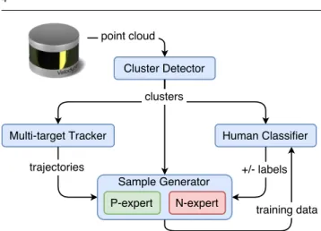
Fig. 2 Process details of the online learning framework.
ronments, and that such an approach provides comparable or superior results with respect to previous methods.
3 General Framework for Online Learning
Our system consists of four main components: a cluster de-tector for 3D LiDAR point clouds, a multi-target tracker, a human classifier and a training sample generator (see Fig. 2). The classifier is initialised by supervised learning with a small set of human clusters. The size of this set could be as small as one, since more samples will be added incre-mentally and used for retraining in future iterations.
The online process works as follows. At each new itera-tion, a 3D LiDAR scan (i.e. 3D point cloud) is segmented by the cluster detector. Positions and velocities of the clusters are estimated in real-time by a multi-target tracking system. These estimates are buffered in trajectory arrays together with their respective cluster observations. At the same time, the classifier labels each cluster as ‘human’ or ‘non-human’. The sample generator exploits all the information about clusters, trajectories and labels. The latter are typically af-fected by two types of errors: false positive and false nega-tive. The sample generator tries to correct them by using two independent “experts”, which cross-check the output of the classifier with that of the tracker. Based on the experts’ de-cisions, the sample generator produces new training data. In particular, the P-expert in Fig. 2 converts false negatives into positive samples, while the N-expert converts false positives into negative samples. When enough new samples have been generated, they are used to retrain the classifier, so the sys-tem can learn and improve from previous errors. The process and the experts are explained in detail in Section 5.2.
Although conceptually similar to a previous tracking-learning-detection framework [20], the proposed systems dif-fers in three key aspects, namely the independence of the tracker from the classifier, the frequency of the training pro-cess, and the implementation of the experts. In particular,
while the performance of the human classifier depends on the reliability of the experts and the tracker, the latter is com-pletely unaffected by the classification performance. This decoupling makes the system modular and potentially appli-cable to alternative classification methods. Also, instead of retraining incrementally from single samples (i.e. frame-by-frame training), our system performs a less frequent batch-incremental training [35] (i.e. gathering samples in batches to retrain the classifier after a certain period), collecting new data online as the robot moves in the environment. This fea-ture can effectively prevent under-fitting in online learning. Finally, our implementation of the experts is specifically de-signed to deal with more than one target simultaneously, and therefore to generate new training samples from multiple de-tections, speeding up the learning process.
4 Point Cloud Cluster Detection and Tracking
Two key components of the proposed system shown in Fig. 2 are the cluster detector and the multi-target tracker. The for-mer detects, in real-time, clusters of point clouds from 3D Li-DAR data. Their positions and velocities are estimated by the tracker, also in real-time, independently of whether the clusters belong to humans or not. Details about the two mod-ules are provided next.
4.1 Point Cloud Cluster Detector
The input of the cluster detector is a 3D LiDAR point cloud
P={pi |pi= (xi,yi,zi)∈R3, i=1, . . . ,I}, whereIis the total number of points in a single scan. In order to discard points belonging to the floor, the detector removes every pi withzi<zmin, leaving a subsetP∗⊂P. This obviously works well only for relatively flat floors andz-axis roughly perpen-dicular to ground, which is one of our assumptions, and ac-cepting the fact that small lower parts of an object could be discarded. It is however worth noting that the core idea of our proposed clustering algorithm is not subject to ground removal, and other methods could be used for this in more complex situations [13, 30].
As in [36], non-overlapping clusters of adjacent points are extracted based on their 3D Euclidean distance. In partic-ular, ifCi,Cj⊂P∗are two such clusters, the non-overlapping condition can be written as follows:
Ci∩Cj=/0,fori6=j ⇒ minkpi−pjk2≥d∗ (1)
wherepi∈Ci,pj∈Cj, andd∗is a distance threshold. Although relatively fast and simple, distance-based clus-tering can be inaccurate, especially if the density of points in the cloud varies significantly with the distance from the sensor. If the thresholdd∗is too small, single objects could
Fig. 3 Point cloud of two distinct objects (red and blue). Different val-ues ofd∗lead to different clustering results.
Fig. 4 Example of 3D LiDAR human point clouds at different dis-tances. The further the person is from the sensor, the sparser is the relative point cloud.
be split into multiple clusters. If too large, multiple objects could be merged into a single cluster (see Fig. 3).
In our case, the shape of the point clouds formed by 3D LiDAR scans on the human body can vary significantly with the distance of the person from the sensor. In particular, due to its vertical angular resolution (Θ =2◦), the vertical distance between two consecutive points can be very large, as shown in Fig. 4. We therefore adapt the thresholdd∗ to the actual scan rangeras follows:
d∗=2·r·tanΘ
2 (2)
This equation simply computes the expected vertical dis-tance between two adjacent scan channels for some straight vertical object.
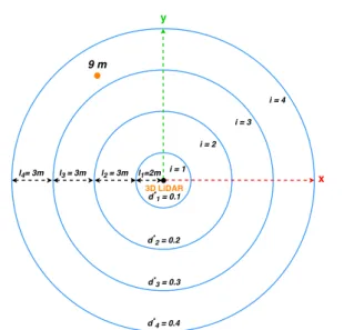
Unfortunately, clustering of 3D points can be computa-tionally intensive. The longer the maximum scan range, the higher the value ofd∗, and therefore the number of points falling within the same cluster. In addition, considering a large area increases the number of potential clusters. To re-duce the complexity, we divide the horizontal space into nested circular regions around the sensor, and fix a constant distance threshold within each of them (see Fig. 5).
In practice, we consider a set of valuesdi∗ at fixed in-tervals ∆d, wheredi+∗1=di∗+∆d. For each of them, we
compute the maximum cluster detection rangeri using the inverse of Equation (2), and determine the corresponding ra-diusRi=bric, whereR0is centre of the sensor. The width
of a region with constant thresholdd∗i isli=Ri−Ri−1. In
Fig. 5 Different values ofd∗correspond to different nested regions. In this example, a cluster (red dot) at 9m from the sensor lies on the 4th circular region, where the clustering threshold isd4∗=0.4m.
our application, we define circular regions 2-3m wide using
∆d=0.1m, which is a good resolution to detect potential
human clusters.
Finally, clusters that are too large or too small to corre-spond to humans are filtered out, so that only the following set of cluster detections is actually used by the tracker:
C={Cj|0.2≤wj≤1, 0.2≤dj≤1,0.2≤hj≤2} (3)
wherewj,djandhjare the width, depth and height (in me-ters), respectively, of the volume containingCj. The time complexity of our proposed clustering algorithm isO(logn)
with an implementation based on ak-d tree.
4.2 Multi-target Tracker
The multi-target tracker is based on an efficient Unscented Kalman Filter (UKF) implementation, using Global Near-est Neighbour (GNN) data association to deal with multiple clusters simultaneously [2, 3]. Human clusters are tracked on a 2D plane, corresponding to a flat floor, estimating horizon-tal coordinates and velocities with respect to a fixed world frame of reference. In the current implementation, the 3D cluster size is not taken into account, although it could prove beneficial in more challenging tracking scenarios.
The prediction step of the estimation is based on the fol-lowing constant velocity model [26]:
xk=xk−1+∆tx˙k−1 ˙ xk=x˙k−1 yk=yk−1+∆ty˙k−1 ˙ yk=y˙k−1 (4)
where xk and yk are the Cartesian coordinates of the tar-get at time tk, ˙xk and ˙yk are the respective velocities, and
∆t=tk−tk−1.
The position of a cluster is computed by projecting onto the(x,y)plane its centroidcj, computed as follows:
cj=
1
|Cj|p
∑
i∈Cj
pi (5)
The update step of the estimation then uses a 2D polar observation model to represent the position of the cluster: θk =tan−1(yk/xk) γk = q x2k+y2k (6)
whereθk andγk are the bearing and the distance, respec-tively, of the cluster from the sensor. Note that noises and coordinate transformations, including those relative to the robot motion, are omitted in the above equations for the sake of simplicity.
The choice of the above models and estimation tech-nique is motivated by the type of sensor used. In particu-lar, the polar observation model better represents the actual functioning of our LiDAR sensor (i.e. the raw measures are range values at regular angular intervals) and its noise prop-erties. The non-linearity of this model leads therefore to the adoption of the UKF, which is known to perform better than a standard EKF [19, 3]. Previous studies [3, 27] showed that our estimation framework is an effective and efficient so-lution to track multiple people with mobile robots. More details about our track management solution (i.e. initialisa-tion, maintenance, deletion) and possible application can be found in [2, 3, 12].
Finally, the covariance matricesQandRof the noises for the prediction and observation models, respectively, are the following [26]: Q= ∆t4 4 σ 2 x ∆t 3 2 σ 2 x 0 0 ∆t3 2 σx2∆t2σx2 0 0 0 0 ∆t4 4 σ 2 y ∆t 3 2 σ 2 y 0 0 ∆t3 2 σ 2 y ∆t2σy2 R= σθ2 0 0 σγ2 (7)
where the noise standard deviationsσx,σy,σθ andσγwere empirically determined to optimize the human tracking per-formance of our robot platform.
5 Online Learning for Human Classification
The point cloud clusters detected in Section 4.1 are anal-ysed, in real-time, by a classifier distinguishing between hu-mans and non-huhu-mans. Our online learning framework is an iterative process in which the classifier is periodically re-trained, online, using old and new cluster detections, which
are provided by the sample generator. The latter selects, based on tracking information, a pre-defined number of positive and negative clusters, and uses them to retrain the human classifier. The classification and sample generation processes are explained in detail in the following sub-sections.
5.1 Human Classifier
A standard Support Vector Machine (SVM) [8] is used for human classification. The SVM method has a solid theoreti-cal foundation in mathematics, which is good at dealing with small data samples and therefore very suitable for our pro-posed online learning framework. Moreoever, this algorithm is known to work well in non-linear classification problems, and has already been applied successfully for 3D LiDAR-based human detection [32, 23].
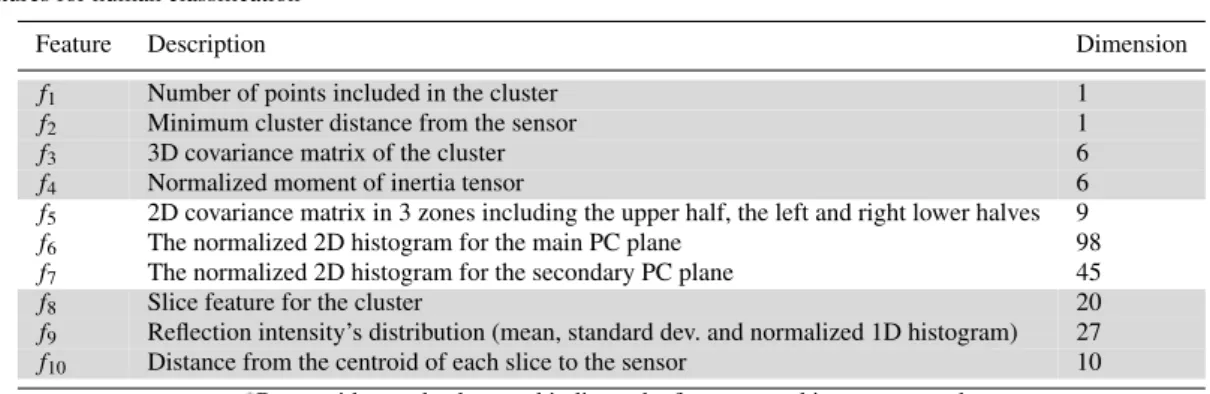
In order to train the SVM, we extract seven different fea-tures from each point cloud cluster, which are shown in Ta-ble 1. Features(f1, . . . ,f7)were proposed by [32]. However,
we discarded the last three because of their heavy computa-tional cost and relatively low classification performance [23], which make them unsuitable for real-time people tracking in large populated environments, and replaced them instead with three different features:f8,f9andf10. The former two, f8andf9were originally proposed by [23]. The combination
of these two features with(f1, . . . ,f4)was shown to
success-fully characterise both standing and sitting people [47]. Feature f10, instead, is a new addition to our system,
which aims at coupling the detection distance of the sensor with the 3D shape of humans, especially for long distance classification with a sparse point cloud. This new feature, called “slice distance”, is based on the 10 slices of [23] and is computed as follows:
f10={kcik2|ci= (xi,yi,zi)∈R3,i=1, . . . ,10} (8) whereci is the centroid of each slice, which can be calcu-lated as in Equation (5). The purpose of the 10 slices was to extract the partial features of humans observed from a long distance, where the spatial resolution of the LiDAR’s point clouds decreases. The 3D points in the cluster are di-vided into 10 blocks, and the length and width of each block are computed as features (see Fig. 6). The respective feature vector is the following:
f8={Lj,Wj| j=1, . . . ,10} (9)
In Section 7.3 we will show that, by using our feature set, the classifier improves on the state-of-the-art.
The full set of features from clusterCj forms a vector
(f1, . . . ,f4,f8, . . . ,f10), with 71 dimensions in total. At each
iteration of the learning process, a binary SVM is trained to label human and non-human clusters based on these fea-tures. The software tool we use is LIBSVM [7], setting the
Table 1 Features for human classification∗
Feature Description Dimension
f1 Number of points included in the cluster 1
f2 Minimum cluster distance from the sensor 1
f3 3D covariance matrix of the cluster 6
f4 Normalized moment of inertia tensor 6
f5 2D covariance matrix in 3 zones including the upper half, the left and right lower halves 9 f6 The normalized 2D histogram for the main PC plane 98 f7 The normalized 2D histogram for the secondary PC plane 45
f8 Slice feature for the cluster 20
f9 Reflection intensity’s distribution (mean, standard dev. and normalized 1D histogram) 27 f10 Distance from the centroid of each slice to the sensor 10
∗Rows with gray background indicate the features used in our approach.
Fig. 6 The slice feature proposed by [23].
ratio of positive and negative training samples to 1 : 1, and scaling all the feature values within the interval[−1,1]. The SVM uses a Gaussian Radial Basis Function kernel [22] and outputs probabilities associated to the labels. Currently our software does not support incremental learning, so it stores all the training samples since the beginning and uses all of them to retrain the SVM at each new iteration. The train-ing/retraining time is proportional to the number of samples. For our experimental configuration in Section 7, it takes from less than 1 millisecond to a few minutes. However, based on our released source code, one can easily decouple the train-ing process from the online learntrain-ing (e.g. by ustrain-ing indepen-dent threads) as needed, or fine-tune the k-fold cross valida-tion (for finding optimal training parameters) to speed up the training process. Moreover, our framework for online learn-ing allows for the implementation of different classifiers and training algorithms.
5.2 Sample Generator
The training samples needed to retrain the human classifier are selected from the current cluster detections by the sam-ple generator in Fig. 2. This is based on two independent modules: a positive (P) expert and a negative (N) expert. At each time step, the P-expert analyses the current clusters
classified as non-humans to identify the potentially incorrect ones (i.e. false negatives). The latter are added to the training set as new positive samples. Conversely, the N-expert exam-ines the current clusters classified as humans, identifies the wrong ones (i.e. false positives), and adds them to training set as new negative samples. This process is repeated several times, until a sufficient number of new positive and negative samples have been collected. Then the human classifier is retrained with the augmented training set. In practice, the P-expert increases the generality of the classifier, while the N-expert increases the discriminability. The implementation details are described in Algorithm 1.
Algorithm 1:Sample Generation and Retraining Data: H: human classifier,C: clusters,
Ch: human clusters,Cn: non-human clusters, Sp: positive samples,Sn: negative samples, Tp: positive training set,Tn: negative training set, p: number of iterative positive training samples, n: number of iterative negative training samples, i: number of iterations,
m: maximum number of iterations Result:H: human classifier Tp←−Sp; Tn←−Sn; train(H,Tp,Tn); i←−1; repeat repeat [Ch,Cn]←−Classi f y(H,C); Sp←−Pexpert(Ch,Cn); Sn←−Nexpert(Ch,Cn); Tp←−Tp+Sp; Tn←−Tn+Sn; until|Tp|>=p∗iand|Tn|>=n∗i; train(H,Tp,Tn); i←−1+1; untili>m;
The P-expert selects new positive samples based on the tracked trajectories of the detected clusters. In particular, clusters classified as non-human, but belonging to a
trajec-Fig. 7 Example of human-like trajectory samples, including one (red-crossed) filtered out because too uncertain. The green dashed line is the target’s trajectory, while the blue dashed circles are the position’s uncertainties.
tory where at least one cluster was classified as human, will be added to the training set as positive samples. The con-ditions to be satisfied by such new positive samples are as follows:
1. the cluster is continuously tracked for the time interval
K∆t, during which it covers a minimum distancerminp :
rk=
q
(xk−xk−1)2+(yk−yk−1)2 and
K
∑
k=1rk≥rminp (10)
2. its velocity is not null but also not faster than a person’s preferred walking speedvmaxp =1.4 m/s [29]:
vk=
q ˙
xk2+y˙2k and vminp ≤vk≤vmaxp (11)
3. the variances(σx2,σy2)of its estimated position(xk,yk) satisfy the following condition:
σx2+σy2≤(σmaxp )2 (12) The values ofK,rminp ,vminp andσmaxp used in our system were empirically tuned before the experiments. The last condi-tion, in particular, is particularly useful to filter out clusters that, even if associated with “human-like” trajectories, have a high level of uncertainty because of sudden movements or the proximity of other clusters (see Fig. 7).
The N-expert analyses clusters classified as humans and selects those which are potential false positives, transform-ing them into new negative samples for future retraintransform-ing. This selection is based on the assumption that humans are
notcompletelystatic, as there are always some changes in
a cluster’s shape and its centroid position, even if the per-son is simply standing or sitting. Taking advantage of the 3D LiDAR’s high accuracy, these static clusters (considered as negative samples) can be identified if they satisfy the fol-lowing conditions:
rk≤rnmax and vk≤vnmax and σx2+σy2≤(σmaxn )2 (13)
The parametersrnmax,vnmax, and σmaxn were determined em-pirically for the experiments. The performance of the P-N experts with respect to the stability of the online learning process is also discussed and evaluated in Section 7.2.
6 System Setup and Dataset
Our framework has been fully implemented into ROS (Robot Operating System) [34] with high modularity. All compo-nents are ready for download2and use by other researchers. We evaluated the framework on a dataset3collected with a mobile robot and a Velodyne VLP-16 3D LiDAR in a large university building.
6.1 Recording Platform
The 3D LiDAR provides 16 scan channels with 360◦ hori-zontal and 30◦vertical field-of-view. The sensor was mounted on the top of a Pioneer 3-AT robot, as shown in Fig. 8. Its supporting frame and placement resemble the design of the industrial cleaning robot developed in the EU project FLOBOT4. The inner mechanism rotates counter-clockwise on its vertical axis, at rates ranging between 300 and 1,200 revolutions per minute (RPM), equivalent to 5 and 20 Hz, re-spectively. The scanning resolution is inversely proportional to the rotation speed. However, changing the spin rate does not change the data rate, because the horizontal angular res-olution is automatically adjusted by the sensor. This means the unit sends out always the same number of packets at a rate of 0.3 million points per second, regardless of the se-lected spin rate.
In our case, the 3D LiDAR was set to rotate at 10 Hz (i.e. 600 RPM) with a maximum scan range of 100 m. The robot maximum speed was set to 2.52 km/h, and the max-imum turning speed to 140◦/s. Both robot and sensor were connected to an embedded PC, mounted on the same plat-form, with an Intel i7-4765T processor and 8GB memory. In addition, a fish-eye camera was mounted on the top of the 3D LiDAR and connected to the PC via WiFi, so panoramic images of the environment around the robot were recorded and used for data annotation5.
All the software for data recording and robot motion was implemented in ROS, running on Linux Ubuntu 14.04 LTS (64-bit). The 3D point clouds were provided by the Velo-dyne’s official ROS driver and calibration file. All data were recorded inrosbagfiles for easy sharing with the robotics
2 https://github.com/LCAS/online_learning
3
http://lcas.lincoln.ac.uk/wp/research/data-sets-software/l-cas-3d-point-cloud-people-dataset/
4 http://www.flobot.eu
5 Due to privacy issues, currently panoramic images are not included in the dataset.
Fig. 8 Our hardware platform, in which the (1) Velodyne VLP-16 3D LiDAR is mounted at 0.8m from the floor, on the top of the Pi-oneer 3-AT robot.
community. Moreover, together with the point cloud data, the robot odometry and the coordinate transformations (sen-sor positions) were also recorded into therosbagfiles. All the data is timestamped, providing essential information for ground-truth where any object (robot, sensor or human) can be accurately localized.
6.2 Data Annotation
We developed an open-source Qt-based tool for data an-notation (see Fig. 9), also available with our dataset. The tool provides a semi-automatic labelling function commonly used by similar 2D image and video annotation software [21, 5]. In our case, the 3D point cloud (from a PCD file6) is first
segmented into candidate clusters to be labelled by a user, who can indicate information such as the candidate’s ID, category (e.g. pedestrian, group7, etc.) and visibility (e.g.
visible or partially visible). The tool allows to modify and add new annotations to previous datasets. It can be also eas-ily extended to label other objects, such as bicycles or cars [42], or to segment and annotate tracklets.
6.3 L-CAS 3D Point Cloud People Dataset
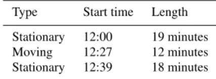
The dataset contains 28,002 scans, recorded with our mo-bile robot, both while moving and stationary in a large and crowded academic building (see Fig. 10), as detailed in ta-ble 2. Each 3D scan contains around 30,000 points. In addi-tion to the X-Y-Z coordinates, each point data includes the
6 http://pointclouds.org/documentation/tutorials/
pcd_file_format.php
7 Although the “group” samples are not used in this paper, these annotations are included in our dataset to be used by other researchers for group tracking or other applications.
Fig. 9 Screenshot of our annotation tool in operation.
Table 2 Overview of our dataset
Type Start time Length Stationary 12:00 19 minutes Moving 12:27 12 minutes Stationary 12:39 18 minutes
scan channel’s number and the intensity of the returned light pulse. The latter is very useful for human classification (see feature f9in Table 1), since each material has a unique
re-flection characteristic in the near-infrared region of the laser beam, which can help distinguish between human bodies (i.e. clothing) and other objects [23].
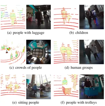
A total of 5,492 scans were manually annotated on the 19 minutes of stationary data, which contains 6,140 human clusters. The minimum and maximum number of 3D points generated by the scan of a person are 3 and 3,925, respec-tively, while the minimum and maximum distance from the sensor are 0.5 m and 27 m, respectively. As shown in Fig. 11, the dataset captures many challenging situations, such as hu-man groups, children, people with trolleys, etc., the combi-nation of which is seldom included in similar datasets.
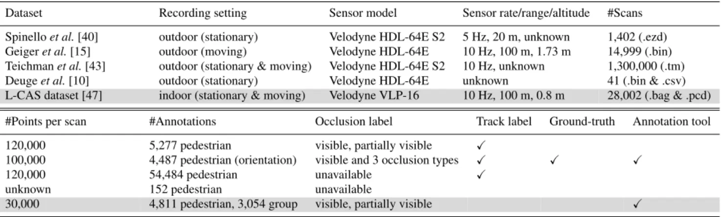
A comparison of our 3D LiDAR dataset with other simi-lar ones can be seen in Table 3. To our knowledge, this is the only such dataset collected indoors with a moving and sta-tionary robot. Although the scan channels and the resolution of the Velodyne VLP-16 are lower than other models, the quality of the data provided by our sensor is perfectly suit-able for most indoor applications, allowing us to detect and track people up to 25 m from the robot. Our dataset provides also the second largest number of laser scans, stored in two file formats, i.e.bag for ROS andpcdfor Point Cloud Li-brary (PCL) [37], which are both very popular in the robotics community.
7 Experimental Results
The experiments reported in this paper were carried out on a laptop with an Intel i7-7560U (2.40GHz) processor and
Fig. 10 Example of annotated laser scan of the academic building. Ground and ceiling points have been removed. Each bounding box represents a cluster, and red boxes are humans. The image contains some typical annotation challenges: (1) human sample at 25 m from the sensor consisting of 5 points only; (2) cluster of a sitting person, included the chair; (3) cluster of two people sitting at a circular table, who cannot be labelled as a humans; (4) human head only, the rest of the body is occluded; (5) clusters of people with many occlusions.
Table 3 Comparison of existing 3D LiDAR datasets.
Dataset Recording setting Sensor model Sensor rate/range/altitude #Scans Spinelloet al.[40] outdoor (stationary) Velodyne HDL-64E S2 5 Hz, 20 m, unknown 1,402 (.ezd) Geigeret al.[15] outdoor (moving) Velodyne HDL-64E 10 Hz, 100 m, 1.73 m 14,999 (.bin) Teichmanet al.[43] outdoor (stationary & moving) Velodyne HDL-64E S2 10 Hz, unknown 1,300,000 (.tm) Deugeet al.[10] outdoor (stationary) Velodyne HDL-64E unknown 41 (.bin & .csv) L-CAS dataset [47] indoor (stationary & moving) Velodyne VLP-16 10 Hz, 100 m, 0.8 m 28,002 (.bag & .pcd) #Points per scan #Annotations Occlusion label Track label Ground-truth Annotation tool 120,000 5,277 pedestrian visible, partially visible X
100,000 4,487 pedestrian (orientation) visible and 3 occlusion types X X X
120,000 54,484 pedestrian unavailable X
unknown 152 pedestrian unavailable
30,000 4,811 pedestrian, 3,054 group visible, partially visible X
16GB memory (Ubuntu 16.04 64-bit + ROS Kinetic) for the comparison of the clustering precision and runtime as well as the online classification under uncertainty, and a lap-top with an Intel i7-6560U (2.20GHz) processor and 8GB memory (Ubuntu 14.04 64-bit + ROS Indigo) for the rest. Experiments for evaluating the clustering performance were run using only one core of the CPU.
7.1 Clustering Performance
The first experiment evaluated the runtime performance of our point cloud clustering algorithm. We used the 19 min-utes of data for the stationary case, and reported the op-erating frequency at different detection distances. The re-sults in Fig. 12 shows that the frequency decreases as the distance increases, in particular during the first few meters, where there is a large drop from ~50 Hz to ~20 Hz. This is due to the fact that the greater the distance from the sensor,
the more laser points are considered. In particular, there are fewer obstacles (e.g. pedestrians) within the first few me-ters, and therefore fewer laser beams reflected by them that are taken into account by the clustering algorithm. Due to some code optimization, the results are also much improved in comparison to our previous work [47] and show that our clustering frequency is well above the minimum 5 Hz typi-cally required for human tracking [3].
We then compared our approach against the current state-of-the-art in terms of precision and runtime. For the former, we considered a large open space, where a person walked towards the 3D LiDAR starting at 25 m and finishing at 1 m from the sensor, while a second person walked from one side to another at 19 m and 11 m, respectively, from the sensor. Fig. 13 depicts a moment of the experimental scenario. The whole process took 17 seconds, with the 3D LiDAR running at 10 Hz. In total, 172 scans were acquired and subsequently
(a) people with luggage (b) children
(c) crowds of people (d) human groups
(e) sitting people (f) people with trolleys Fig. 11 Different challenging scenarios captured by our dataset.
0 10 20 30 40 50 60 70 80 90 100 110 2m 5m 8m 11m 14m 17m 20m 22m 25m 28m 31m frequency [Hz] distance [m] 53.0 20.9 20.1 20.1 19.5 19.2 18.9 18.7 18.6 18.5 18.3
Fig. 12 Runtime performance of the clustering algorithm varying the maximum LiDAR detection range. For example, 2mrefers only to the measurements (points) within this particular distance. The respective mean is shown on the top of each box. As one can see, the amount of clutter (and therefore detected clusters) is inversely proportional to the considered distance from the sensor. This is consistent with the complexity of the algorithm, i.e.O(logn).
fully labelled8to analyse the precision of the cluster
detec-tor.
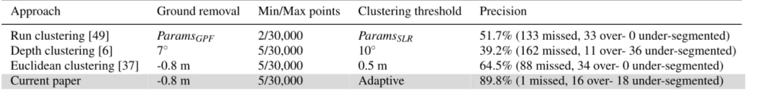
We compared our method to the run-based clustering in [49], depth clustering in [6], and the Euclidean clustering of PCL [37], evaluating the segmentation precision on the above labelled scans. In particular, we counted how many human clusters were correctly segmented, noting “missed” if no clusters were present, “over-segmented” if a person’s point cloud was split into multiple clusters, and “under-segmented” if the cluster size exceeded 30% of the manually labelled one. The parameters of four clustering algorithms and re-8 The data is available at:https://github.com/LCAS/cloud_
annotation_tool
Fig. 13 Two people walking in proximity of the robot in a large open space, one towards the robot and another one from side to side.
sults are shown in Table 4. For the run-based method, we used the parameter values reported in [49]. For the depth and the Euclidean methods, we used the thresholds reported to give the best performance [6]. Note that the main reason for the low performance of the depth clustering is that the latter is based on a 2D range image, where points are clus-tered based on the angle between laser beams. This makes it difficult to distinguish between objects that are very close in depth, or relatively small objects against larger ones in the background, affecting in particular the detection of per-son 2 in the experiment. As shown by the table, instead, our method can handle almost all of these situations, giving a precision which is generally much higher than that of the other approaches.
Regarding runtime performance, we tested the same four methods on the first 2,500 scans of the 19 minutes of data for the stationary robot. The results in Fig. 14 show that the run clustering, depth clustering and our method are an or-der of magnitude faster than the Euclidean approach. The run method is slightly faster than the depth one given the fact that relatively more points were removed along with the ground in its first step, winning the time required for the sec-ond step of clustering. The run method is three times and the depth method is twice as fast as ours, but at the expense of precision, as previously demonstrated.
From the above experiments we can draw the follow-ing conclusion. The run and the depth methods consider the clustering from the perspective of 2D images, while we di-rectly process the 3D point cloud. This results in the first two methods being faster but not accurate enough, while ours is relatively slower but obtains higher precision.
7.2 Stability Analysis
A stability analysis of the learning process is possible by considering the variations of false positivesαand false
neg-Table 4 Parameter settings and segmentation precision of four different methods.
Approach Ground removal Min/Max points Clustering threshold Precision
Run clustering [49] ParamsGPF 2/30,000 ParamsSLR 51.7% (133 missed, 33 over- 0 under-segmented) Depth clustering [6] 7◦ 5/30,000 10◦ 39.2% (162 missed, 11 over- 36 under-segmented) Euclidean clustering [37] -0.8 m 5/30,000 0.5 m 64.5% (88 missed, 34 over- 0 under-segmented) Current paper -0.8 m 5/30,000 Adaptive 89.8% (1 missed, 16 over- 18 under-segmented) ParamsGPF={Nsegs=3,Niter=3,NLPR=20,T hseeds=0.4m,T hdist=0.2m}
ParamsSLR={T hrun=0.5m,T hmerge=1m}
0 200 400 600 800 1000 1200 1400 1600 1800 0 500 1000 1500 2000 2500 runtime [ms] frame number
run clustering (Zermas'17): 25.0 ms +/- 8.4 ms depth clustering (Bogoslavskyi'16): 35.2 ms +/- 7.4 ms Euclidean clustering (PCL): 298.5 ms +/- 162.8 ms our approach: 74.4 ms +/- 16.4 ms
Fig. 14 Runtime performance of the four clustering methods.
ativesβ generated by the human classifier [20]:
αk+1 βk+1 = " 1−R− 1−PP++R+ 1−P− P− R − 1−R+ # × αk βk (14)
wherekindicates the training iteration, whileP+,R+,P−
and R− are the P-precision, P-recall, precision and N-recall of the experts, respectively. The recursive equation in (14) is a discrete dynamical system that can be written asxk+1=M xk. It can be shown that, if the eigenvaluesλ1
andλ2ofMare less than one, thenxconverges to zero.
An interesting observation by looking at (14) is that, if
P+=P−=1, thenMbecomes a diagonal matrix, and there-fore its eigenvalues are simplyλ1=1−R−andλ2=1−R+.
In this case, even a small recall for both experts is sufficient to guaranteeλ1<1 andλ2<1, and therefore the stability
of the learning process. According these criteria, we use the following performance metrics for the P-N experts:
- Precision of P-expert P+=n+t /(nt++n+f)
- Recall of P-expert R+=n+t /β
- Precision of N-expert P−=n−t /(nt−+n−f)
- Recall of N-expert R−=n−t /α
(15)
wheren+t andn+f are the number of true and false positives, respectively, by the P-expert, whilent−andn−f are those by the N-expert. Theα false positives by the human classifier are the total number of instances that should be corrected by the N-expert. Equally, the β false negatives by the human
Table 5 Performance analysis of the P-N experts.
Retrain the classifier every 5 positives and 5 negatives P-expert N-expert Eigenvalues
P+ R+ P− R− λ1 λ2
1.0 0.714 1.0 0.0215 0.9785 0.286 Retrain the classifier every 10 positives and 10 negatives
P-expert N-expert Eigenvalues
P+ R+ P− R− λ
1 λ2
1.0 0.8857 1.0 0.0405 0.9595 0.1143 Retrain the classifier every 20 positives and 20 negatives
P-expert N-expert Eigenvalues
P+ R+ P− R− λ1 λ2
1.0 1.0 1.0 0.0271 0.9729 0
classifier are the total number of instances that should be corrected by the P-expert.
Table 5 shows the results for 10 training iterations per-formed on the same 172 scans of the previous experiment. Three classifiers were manually initialised using just one sample, and then retrained every 5, 10 or 20 new positives and an equal number of negative samples, respectively. In this way, the stability of our online learning was verified also for different training intervals. As we can see, the perfor-mance of both experts is generally good. In particular, since
P+=P−=1 and alsoR+>0 ∧ R−>0, the stability of the online learning is always guaranteed by the eigenvalues
λ1<1 ∧ λ2<1, as discussed above.
7.3 Classification Performance
In this section we evaluate the performance of the 3D LiDAR-based human classifier, first by analysing the classification results of the SVM trained online and offline, then by assess-ing the online trained SVM under uncertainty, and finally by comparing the results with our new feature set against other state-of-the-art feature combinations.
7.3.1 Online Versus Offline Classification
We first compared the SVM classifier, trained online by our system, versus the same classifier trained offline with man-ually labelled data. In order to illustrate the improvement
gained over time by the former, the performance at the be-ginning and end of the online training is considered. The offline classifier was trained using 1,000 single-person sam-ples from annotated data, with an equal amount of randomly selected background samples. The online classifier was ini-tially trained with 5 positive and 5 negative samples, cho-sen manually, and then retrained automatically by the sys-tem every 100 positive and 100 negative samples, until the final version had been trained by 1,005 positives and 1,005 negatives.
The test set included 50 scans randomly selected from the 18 minutes of our stationary robot dataset (excluding the scans used to manually train the offline classifier). Both standing and sitting people were added to this set. In partic-ular, it contains 567 single persons with respective clusters containing between 5 and 2,122 points, at a varying distance of 0.5 m to 25 m from the sensor.
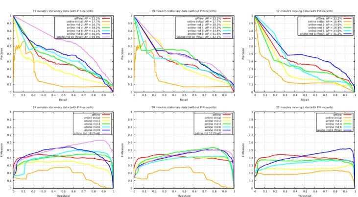
The classification performance was evaluated using stan-dard metrics [14] including Precision, Recall, Average Pre-cision (AP) and F-measure. A human cluster was considered a true positive if the area of overlap between the predicted and the ground-truth bounding boxes was more than 50%. The results are shown in Fig. 15 (the left column), where the improvement of the final online classifier compared to the initial one is evident. Most importantly, the graph shows that the final online classifier outperforms the one trained manu-ally offline. This is largely due to the fact that our tracking system is robust enough to facilitate the detection of clusters far away from the robot, even when these are very difficult for a human annotator to spot, to the benefit of our online learning framework.
7.3.2 Online Classification Under Uncertainty
We then trained a classifier online with the same settings as in Section 7.3.1 but without the P-N experts. Only hu-man trajectories that satisfy Equations 10, 11 and 12 are learned as positives samples. The negatives samples are ran-domly selected background samples. The idea is to report on experiments when the P-expert and N-expert fail, and as a consequence the SVM is retrained with a given number of false positives and false negatives. The results are shown in Fig. 15 (the middle column). As we can see, the classi-fication performance is improved as the number of training rounds increases. However, without the help of the experts to correct the errors online, the improvement is slow and limited.
Another experiment was conducted on the 12 minutes of moving data. We ran the full system (i.e. with the P-N ex-perts) and fine-tuned the parameters described in Section 5.2 to cope with the increased noise generated with the robot moving. A classifier was trained online with 8 rounds and we report its performance on even training rounds, as shown
in Fig. 15 (the right column). As we can see, the classifi-cation performance is improved within our online learning framework but affected by noise. However, it is worth point-ing out that in this experiment the trackpoint-ing system provides the 2D position of people relative to the robot’s odometry, in which drift errors are accumulated. Using LiDAR odometry or map-based localization would improve the current results.
7.3.3 Feature Sets Comparison
Finally, four classifiers with different feature sets were eval-uated in this experiment to demonstrate the improvement generated by our new slice distance featuref10. The four sets
are(f1, . . . ,f7)as proposed by [32],(f1, . . . ,f9)by [23], our
previous set(f1, . . . ,f4,f8,f9)in [47], and finally the current (f1, . . . ,f4,f8, . . . ,f10).
For training, both (positive) human and (negative) back-ground samples were taken from the 19 minutes of station-ary robot data, starting with 5 positives and 5 negatives for the initial supervised stage. The classifiers were retrained every 100 positive and 100 negative samples by our online learning framework, until reaching 1,005 positives and an equal amount of negatives. The final classifiers were then evaluated on the same test set used in the previous experi-ment, with 567 human clusters extracted from the 18 min-utes of stationary robot data, including both standing and sitting people at a varying distance from the sensor.
The results are illustrated in Fig. 16, showing that the AP of our new classifier, enhanced by the proposed slice distance feature, is significantly better than our previous so-lution and, in general, is similar to the other two classifiers. However, instead of using features(f5, . . . ,f7)based on
pro-jected planes with 152 dimensions, our L2 distance-based feature f10, with only 10 dimensions, can significantly
im-prove the system performance, and so it is more suitable for real-time human detection. Also, the Precision-Recall and the F-Measure of our new classifier are generally better than that of the others.
8 Conclusions
This paper presented an improved online learning frame-work for human detection in 3D LiDAR scans, including an extensive evaluation of runtime performance, stability, and classification results. The framework relies on a multi-target tracking system with a real-time clustering algorithm and an efficient sample generator. It enables a mobile robot to learn autonomously from the environment what humans look like, which greatly reduces the need for tedious and time-consuming data annotation.
We showed that our adaptive clustering method is more precise than other state-of-the-art algorithms, while still main-taining a low computational cost suitable for most human
0 0.1 0.2 0.3 0.4 0.5 0.6 0.7 0.8 0.9 1 0 0.1 0.2 0.3 0.4 0.5 0.6 0.7 0.8 0.9 1 P recision Recall
19 minutes stationary data (with P-N experts)
offline: AP = 33.2% online initial: AP = 17.7% online rnd 2: AP = 26.7% online rnd 4: AP = 38.2% online rnd 6: AP = 41.1% online rnd 8: AP = 46.9% online rnd 10 (final): AP = 59.8% 0 0.1 0.2 0.3 0.4 0.5 0.6 0.7 0.8 0.9 1 0 0.1 0.2 0.3 0.4 0.5 0.6 0.7 0.8 0.9 1 P recision Recall
19 minutes stationary data (without P-N experts)
offline: AP = 33.2% online initial: AP = 17.7% online rnd 2: AP = 30.2% online rnd 4: AP = 35.2% online rnd 6: AP = 34.4% online rnd 8: AP = 41.5% online rnd 10 (final): AP = 42.1% 0 0.1 0.2 0.3 0.4 0.5 0.6 0.7 0.8 0.9 1 0 0.1 0.2 0.3 0.4 0.5 0.6 0.7 0.8 0.9 1 P recision Recall 12 minutes moving data (with P-N experts)
offline: AP = 33.2% online initial: AP = 16.4% online rnd 2: AP = 24.0% online rnd 4: AP = 28.4% online rnd 6: AP = 34.0% online rnd 8 (final): AP = 41.2% 0 0.1 0.2 0.3 0.4 0.5 0.6 0.7 0.8 0.9 1 0 0.1 0.2 0.3 0.4 0.5 0.6 0.7 0.8 0.9 1 F-Measur e Threshold 19 minutes stationary data (with P-N experts)
offline online initial online rnd 2 online rnd 4 online rnd 6 online rnd 8 online rnd 10 (final) 0 0.1 0.2 0.3 0.4 0.5 0.6 0.7 0.8 0.9 1 0 0.1 0.2 0.3 0.4 0.5 0.6 0.7 0.8 0.9 1 F-Measur e Threshold
19 minutes stationary data (without P-N experts) offline online initial online rnd 2 online rnd 4 online rnd 6 online rnd 8 online rnd 10 (final) 0 0.1 0.2 0.3 0.4 0.5 0.6 0.7 0.8 0.9 1 0 0.1 0.2 0.3 0.4 0.5 0.6 0.7 0.8 0.9 1 F-Measur e Threshold 12 minutes moving data (with P-N experts)
offline online initial online rnd 2 online rnd 4 online rnd 6 online rnd 8 (final)
Fig. 15 Performance evaluation of the 3D LiDAR-based human classifier. Left column: online versus offline classification. Middle column: online classification without P-N experts. Right column: online classification with robot moving. The initial online classifiers are trained with manually chosen 5 positive and 5 negative samples.
tracking applications. The stability of the online learning process has been analysed in detail, and has been guaranteed in practice by the high-precision of our P-N expert mod-ules in providing good training samples. Our experiments showed also that, thanks to an augmented set of efficient fea-tures, our human classifier performs better than other state-of-the-art solutions in terms of F-measure (accuracy), but with comparable precision and recall.
The whole system is implemented in ROS following a modular design. Both the software and the dataset used in our experiments are publicly available for research purposes. Although currently used for human detection and tracking, our software could be extended to deal with other moving objects such as cars, bicycles or animals [42]. The 3D LiDAR-based cluster detection module could also be replaced by other detectors based on different sensors, such as RGB-D cameras and 2D LiDARs [48].
Future extensions should include coupling the human classifier to the multi-target tracker, so that improving the classification of human clusters also improves people track-ing. Moreover, although our solution enables human detec-tion with mobile robots in dynamic environments, in the current paper it has been tested only on datasets recorded for relatively short period of times. Daily routines in pub-lic environments could be exploited by a service robot, for example, to collect negative background samples at night, when there are no moving objects, and positive human
sam-ples during the day9. Long-term operation and open-ended learning are therefore two promising directions for future re-search in this area [45]. Future work should look at other classification methods such as deep neural networks, ex-ploiting online learning to overcome the difficulty of col-lecting extensive training samples.
References
1. Arras, K.O., Mozos, O.M., Burgard, W.: Using boosted features for the detection of people in 2d range data. In: Proceedings of the 2007 IEEE International Conference on Robotics and Automation (ICRA), pp. 3402–3407 (2007)
2. Bellotto, N., Hu, H.: Multisensor-based human detection and tracking for mobile service robots. IEEE Transactions on Sys-tems, Man, and Cybernetics – Part B39(1), 167–181 (2009) 3. Bellotto, N., Hu, H.: Computationally efficient solutions for
track-ing people with a mobile robot: an experimental evaluation of bayesian filters. Autonomous Robots28, 425–438 (2010) 4. Beyer, L., Hermans, A., Linder, T., Arras, K.O., Leibe, B.: Deep
person detection in two-dimensional range data. IEEE Robotics and Automation Letters3(3), 2726–2733 (2018)
5. Bianco, S., Ciocca, G., Napoletano, P., Schettini, R.: An interac-tive tool for manual, semi-automatic and automatic video anno-tation. Computer Vision and Image Understanding131, 88–99 (2015)
6. Bogoslavskyi, I., Stachniss, C.: Fast range image-based segmen-tation of sparse 3d laser scans for online operation. In: Proceed-ings of the 2016 IEEE/RSJ International Conference on Intelligent Robots and Systems (IROS), pp. 163–169 (2016)
9 Dataset collection is also in progress at University of Lincoln and at University of Technology of Belfort-Montb´eliard.
0 0.1 0.2 0.3 0.4 0.5 0.6 0.7 0.8 0.9 1 0 0.1 0.2 0.3 0.4 0.5 0.6 0.7 0.8 0.9 1 P recision Recall f1-f7 (Navarro-Serment'09): AP = 61.0% f1-f9 (Kidono'11): AP = 59.1% f1-f4, f8-f9 (Yan'17): AP = 54.4% f1-f4, f8-f10 (our approach): AP = 59.8% 0 0.1 0.2 0.3 0.4 0.5 0.6 0.7 0.8 0.9 1 0 0.1 0.2 0.3 0.4 0.5 0.6 0.7 0.8 0.9 1 F-Measur e Threshold f1-f7 (Navarro-Serment'09) f1-f9 (Kidono'11) f1-f4, f8-f9 (Yan'17) f1-f4, f8-f10 (our approach)
Fig. 16 Performance evaluation of different human classifiers.
7. Chang, C.C., Lin, C.J.: LIBSVM: A library for support vector ma-chines. ACM Transactions on Intelligent Systems and Technology 2, 1–27 (2011)
8. Cortes, C., Vapnik, V.: Support-vector networks. Machine Learn-ing20(3), 273–297 (1995)
9. Dequaire, J., Ondruska, P., Rao, D., Wang, D., Posner, I.: Deep tracking in the wild: End-to-end tracking using recurrent neural networks. International Journal of Robotics Research (IJRR) pp. 1–21 (2017)
10. Deuge, M.D., Quadros, A., Hung, C., Douillard, B.: Unsupervised feature learning for classification of outdoor 3d scans. In: Proceed-ings of the Australasian Conference on Robotics and Automation (ACRA) (2013)
11. Dewan, A., Caselitz, T., Tipaldi, G.D., Burgard, W.: Motion-based detection and tracking in 3D LiDAR scans. In: Proceedings of the 2016 IEEE International Conference on Robotics and Automation (ICRA), pp. 4508–4513 (2016)
12. Dondrup, C., Bellotto, N., Jovan, F., Hanheide, M.: Real-time multisensor people tracking for human-robot spatial interaction. In: Proceedings of the 2015 IEEE International Conference on Robotics and Automation (ICRA), Workshop on Machine Learn-ing for Social Robotics (2015)
13. Douillard, B., Underwood, J.P., Kuntz, N., Vlaskine, V., Quadros, A.J., Morton, P., Frenkel, A.: On the segmentation of 3d LIDAR point clouds. In: Proceedings of the 2011 IEEE International
Conference on Robotics and Automation (ICRA), pp. 2798–2805 (2011)
14. Everingham, M., Gool, L.J.V., Williams, C.K.I., Winn, J.M., Zis-serman, A.: The pascal visual object classes (VOC) challenge. In-ternational Journal of Computer Vision88, 303–338 (2010) 15. Geiger, A., Lenz, P., Urtasun, R.: Are we ready for autonomous
driving? the KITTI vision benchmark suite. In: Proceedings of the 2012 IEEE Conference on Computer Vision and Pattern Recogni-tion (CVPR), pp. 3354–3361 (2012)
16. Gonz´alez, A., Villalonga, G., Xu, J., V´azquez, D., Amores, J., L´opez, A.M.: Multiview random forest of local experts combining RGB and LIDAR data for pedestrian detection. In: Proceedings of the 2015 IEEE Intelligent Vehicles Symposium (IV), pp. 356–361 (2015)
17. H¨aselich, M., J¨obgen, B., Wojke, N., Hedrich, J., Paulus, D.: Confidence-based pedestrian tracking in unstructured environ-ments using 3d laser distance measureenviron-ments. In: Proceedings of the 2014 IEEE/RSJ International Conference on Intelligent Robots and Systems (IROS), pp. 4118–4123 (2014)
18. Jafari, O.H., Mitzel, D., Leibe, B.: Real-time RGB-D based peo-ple detection and tracking for mobile robots and head-worn cam-eras. In: Proceedings of the 2014 IEEE International Conference on Robotics and Automation (ICRA), pp. 5636–5643 (2014) 19. Julier, S.J., Uhlmann, J.K.: Unscented filtering and nonlinear
esti-mation. Proc. of the IEEE92(3), 401–422 (2004)
20. Kalal, Z., Mikolajczyk, K., Matas, J.: Tracking-learning-detection. IEEE Transactions on Pattern Analysis and Machine Intelligence 34, 1409–1422 (2012)
21. Kavasidis, I., Palazzo, S., Salvo, R.D., Giordano, D., Spampinato, C.: A semi-automatic tool for detection and tracking ground truth generation in videos. In: Proceedings of the 1st International Workshop on Visual Interfaces for Ground Truth Collection in Computer Vision Applications (2012)
22. Keerthi, S.S., Lin, C.J.: Asymptotic behaviors of support vector machines with gaussian kernel. Neural Computation15(7), 1667– 1689 (2003)
23. Kidono, K., Miyasaka, T., Watanabe, A., Naito, T., Miura, J.: Pedestrian recognition using high-definition LIDAR. In: Proceed-ings of the 2011 IEEE Intelligent Vehicles Symposium (IV), pp. 405–410 (2011)
24. Leigh, A., Pineau, J., Olmedo, N.A., Zhang, H.: Person track-ing and followtrack-ing with 2d laser scanners. In: Proceedtrack-ings of the 2015 IEEE International Conference on Robotics and Automation (ICRA), pp. 726–733 (2015)
25. Li, K., Wang, X., Xu, Y., Wang, J.: Density enhancement-based long-range pedestrian detection using 3-d range data. IEEE Transactions on Intelligent Transportation Systems17, 1368–1380 (2016)
26. Li, X.R., Jilkov, V.P.: Survey of maneuvering target tracking. part i: Dynamic models. IEEE Trans. on Aerospace and Electronic Systems39(4), 1333–1364 (2003)
27. Linder, T., Breuers, S., Leibe, B., Arras, K.O.: On multi-modal people tracking from mobile platforms in very crowded and dy-namic environments. In: Proceedings of the 2016 IEEE Interna-tional Conference on Robotics and Automation (ICRA), pp. 5512– 5519 (2016)
28. Luber, M., Arras, K.O.: Multi-hypothesis social grouping and tracking for mobile robots. In: Proceedings of Robotics: Science and Systems (2013)
29. Mohler, B.J., Thompson, W.B., Creem-Regehr, S.H., Pick, H.L., Warren, W.H.: Visual flow influences gait transition speed and pre-ferred walking speed. Experimental brain research181(2), 221– 228 (2007)
30. Moosmann, F., Pink, O., Stiller, C.: Segmentation of 3d lidar data in non-flat urban environments using a local convexity criterion. In: Proceedings of the 2009 IEEE Intelligent Vehicles Symposium (IV), pp. 1931–0587 (2009)
31. Munaro, M., Menegatti, E.: Fast RGB-D people tracking for ser-vice robots. Autonomous Robots37, 227–242 (2014)
32. Navarro-Serment, L.E., Mertz, C., Hebert, M.: Pedestrian detec-tion and tracking using three-dimensional ladar data. In: Proceed-ings of the 7th Conference on Field and Service Robotics (FSR), pp. 103–112 (2009)
33. Premebida, C., Carreira, J., Batista, J., Nunes, U.: Pedestrian de-tection combining RGB and dense LIDAR data. In: Proceed-ings of the 2014 IEEE/RSJ International Conference on Intelligent Robots and Systems (IROS), pp. 4112–4117 (2014)
34. Quigley, M., Conley, K., Gerkey, B.P., Faust, J., Foote, T., Leibs, J., Wheeler, R., Ng, A.Y.: ROS: an open-source robot operating system. In: ICRA Workshop on Open Source Software (2009) 35. Read, J., Bifet, A., Pfahringer, B., Holmes, G.: Batch-incremental
versus instance-incremental learning in dynamic and evolving data. In: Proceedings of the Eleventh International Symposium on Intelligent Data Analysis (IDA 2012), pp. 313–323 (2012) 36. Rusu, R.B.: Semantic 3D object maps for everyday manipulation
in human living environments. Ph.D. thesis, Computer Science department, Technische Universitaet Muenchen, Germany (2009) 37. Rusu, R.B., Cousins, S.: 3D is here: Point Cloud Library (PCL). In: Proceedings of the 2011 IEEE International Conference on Robotics and Automation (ICRA) (2011)
38. Shackleton, J., Voorst, B.V., Hesch, J.A.: Tracking people with a 360-degree lidar. In: Proceedings of the Seventh IEEE Interna-tional Conference on Advanced Video and Signal Based Surveil-lance (AVSS), pp. 420–426 (2010)
39. Spinello, L., Arras, K.O.: People detection in RGB-D data. In: Proceedings of the 2011 IEEE/RSJ International Conference on Intelligent Robots and Systems (IROS), pp. 3838–3843 (2011) 40. Spinello, L., Luber, M., Arras, K.O.: Tracking people in 3d using
a bottom-up top-down detector. In: Proceedings of the 2011 IEEE International Conference on Robotics and Automation (ICRA), pp. 1304–1310 (2011)
41. Sun, L., Yan, Z., Mellado, S.M., Hanheide, M., Duckett, T.: 3DOF pedestrian trajectory prediction learned from long-term au-tonomous mobile robot deployment data. In: In Proceedings of the 2018 IEEE International Conference on Robotics and Automation (ICRA). Brisbane, Australia (2018)
42. Sun, L., Yan, Z., Zaganidis, A., Zhao, C., Duckett, T.: Recurrent-octomap: Learning state-based map refinement for long-term se-mantic mapping with 3-d-lidar data. IEEE Robotics and Automa-tion Letters3(4), 3749–3756 (2018)
43. Teichman, A., Levinson, J., Thrun, S.: Towards 3d object recog-nition via classification of arbitrary object tracks. In: Proceedings of the 2011 IEEE International Conference on Robotics and Au-tomation (ICRA), pp. 4034–4041 (2011)
44. Teichman, A., Thrun, S.: Tracking-based semi-supervised learn-ing. International Journal of Robotics Research (IJRR) 31(7), 804–818 (2012)
45. Vintr, T., Yan, Z., Duckett, T., Krajnik, T.: Spatio-temporal repre-sentation for long-term anticipation of human presence in service robotics. In: Proceedings of the 2018 IEEE International Con-ference on Robotics and Automation (ICRA). Montreal, Canada (2019)
46. Wang, D.Z., Posner, I.: Voting for voting in online point cloud ob-ject detection. In: Proceedings of Robotics: Science and Systems (2015)
47. Yan, Z., Duckett, T., Bellotto, N.: Online learning for human clas-sification in 3D LiDAR-based tracking. In: In Proceedings of the 2017 IEEE/RSJ International Conference on Intelligent Robots and Systems (IROS). Vancouver, Canada (2017)
48. Yan, Z., Sun, L., Duckett, T., Bellotto, N.: Multisensor online transfer learning for 3d lidar-based human detection with a mo-bile robot. In: Proceedings of the 2018 IEEE/RSJ International Conference on Intelligent Robots and Systems (IROS). Madrid, Spain (2018)
49. Zermas, D., Izzat, I., Papanikolopoulos, N.: Fast segmentation of 3d point clouds: A paradigm on lidar data for autonomous vehicle applications. In: Proceedings of the 2018 IEEE International Con-ference on Robotics and Automation (ICRA). Singapore (2017) 50. Zhou, Y., Tuzel, O.: Voxelnet: End-to-end learning for point cloud
based 3d object detection. In: Proceedings of the 2018 IEEE Con-ference on Computer Vision and Pattern Recognition (CVPR), pp. 4490–4499 (2018)