Graph homomorphisms between trees
P´eter Csikv´ari
Department of Mathematics, Massachusetts Institute of Technology Cambridge, MA 02139
Department of Computer Science, E¨otv¨os Lor´and University H-1117 Budapest, P´azm´any P´eter s´et´any 1/C, Hungary
Zhicong Lin
Department of Mathematics and Statistics, Lanzhou University Lanzhou 730000, P.R. China
Institut Camille Jordan, Universit´e Claude Bernard Lyon 1 43 boulevard du 11 novembre 1918, F-69622 Villeurbanne, France
Submitted: Feb 8, 2014; Accepted: Sep 26, 2014; Published: Oct 9, 2014 Mathematics Subject Classifications: 05C05, 05C30, 05C35
Abstract
In this paper we study several problems concerning the number of homomor-phisms of trees. We begin with an algorithm for the number of homomorhomomor-phisms from a tree to any graph. By using this algorithm and some transformations on trees, we study various extremal problems about the number of homomorphisms of trees. These applications include a far reaching generalization and a dual of Bollob´as and Tyomkyn’s result concerning the number of walks in trees.
Some other main results of the paper are the following. Denote by hom(H, G) the number of homomorphisms from a graphH to a graphG. For any tree Tm on m vertices we give a general lower bound for hom(Tm, G) by certain entropies of
Markov chains defined on the graphG. As a particular case, we show that for any graphG,
exp(Hλ(G))λm−1 6hom(Tm, G),
where λ is the largest eigenvalue of the adjacency matrix of G and Hλ(G) is a
certain constant depending only on Gwhich we call the spectral entropy of G. We also show that if Tm is any fixed tree and
hom(Tm, Pn)>hom(Tm, Tn),
for some treeTnonnvertices, thenTnmust be the tree obtained from a pathPn−1 by attaching a pendant vertex to the second vertex ofPn−1.
All the results together enable us to show that among all trees with fixed number of vertices, the path graph has the fewest number of endomorphisms while the star graph has the most.
Keywords: trees; walks; graph homomorphisms; adjacency matrix; extremal prob-lems; KC-transformation; Markov chains
1
Introduction
We use standard notations and terminology of graph theory, see for instance [2,4]. The graphs considered here are finite and undirected without multiple edges and loops. Given a graphG, we writeV(G) for the vertex set andE(G) for the edge set. Ahomomorphism
from a graph H to a graph G is a mapping f : V(H) → V(G) such that the images of adjacent vertices are adjacent. Let Hom(H, G) denote the set of homomorphisms from
H to G and by hom(H, G) the number of homomorphisms from H to G. Throughout
this article, we write Pn and Sn for the path and the star onn vertices, respectively. The length of a path is the number of its edges. The union of graphs G and H is the graph
G∪H with vertex set V(G)∪V(H) and edge setE(G)∪E(H). A tree T together with a root vertex v will be denoted by T(v).
The problem of computing hom(H, G) is difficult in general. However, there has been recent interest in counting homomorphisms between special graphs. In particular, formulas for computing the number of homomorphisms between two different paths were given in [1,16]. But even for these special trees, the formulas are bulky and inelegant. In Section 2, we shall give an algorithm for computing the number of homomorphisms from trees to any graph. This algorithm will be called Tree-walk algorithm.
Recently, the first author proved a conjecture of Nikiforov concerning the number of closed walks on trees. He proved in [6] that, for a fixed integer m, the number of closed walks of lengthmon trees of ordern attains its maximum at the starSnand its minimum at the path Pn. In other words,
hom(Cm, Pn)6hom(Cm, Tn)6hom(Cm, Sn), (1.1)
where Tn is a tree on n vertices and Cm is the cycle onm vertices.
Bollob´as and Tyomkyn [3] gave a variant of the first author’s result by replacing the number of closed walks by the number of all walks, that is
hom(Pm, Pn)6hom(Pm, Tn)6hom(Pm, Sn), (1.2)
where Tn is a tree on n vertices. In both [3] and [6], the authors use a certain transfor-mation of trees. In [6], it is called thegeneralized tree shift, whereas in [3], it is renamed
toKC-transformation.
To define this transformation, let x and y be two vertices of a tree T such that every interior vertex of the unique x–y path P in T has degree two, and write z for the neighbor of y on this path. Let N(v) denote the set of neighbors of a vertex v. The
k k−1 . . . k−1 k B A B A x z y x y 0 1 0 1
Figure 1: The KC-transformation.
KC-transformation, KC(T, x, y), of the tree T with respect to the path P is obtained fromT by deleting all edges betweeny and N(y)\z and adding the edges between xand
N(y)\z instead (See Fig.1). Note that KC(T, x, y) and KC(T, y, x) are isomorphic. The following property of KC-transformation was proved in [6].
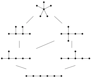
Proposition 1.1. The KC-transformation gives rise to a graded poset of trees on n ver-tices (graded by the number of leaves) with the star as the largest and the path as the
smallest element. See Figure 2.
Figure 2: The induced poset of KC-transformation on trees of 6 vertices.
In [6] the first author proved that the KC-transformation increases the number of closed walks of fixed length in trees. By Proposition 1.1, this leads to the proof of inequality (1.1).
In the very same spirit, Bollob´as and Tyomkyn [3] showed that the KC-transformation increases the number of walks of fixed length in trees. In the language of graph homo-morphism, their result can be restated as follows.
Theorem 1.2 (Bollob´as–Tyomkyn). Let T be a tree and let T′ be obtained from T by a
KC-transformation. Then
hom(Pm, T′)>hom(Pm, T) (1.3)
for any m>1.
Now a natural question arises: does inequality (1.3) still hold when Pm is replaced by an arbitrary fixed tree? A tree is called starlike if it has at most one vertex of degree greater than two. Note that paths are starlike. We answer this question in the affirmative for starlike trees.
Theorem 1.3. Let T be a tree and T′ the KC-transformation ofT with respect to a path
of length k. Then the inequality
hom(H, T′)>hom(H, T) (1.4)
holds when k is even and H is any tree, or k is odd and H is a starlike tree.
Moreover, we find a counterexample for inequality (1.4) when k is odd and H is not a starlike tree (see the end of Section 3).
Another extremal problem concerning the number of homomorphisms between trees that worth considering is to find the extremal trees for hom(·, Pn) over all trees on m
vertices. We address this question in a follow-up paper [8], here we only mention the main result of this paper. This result can be considered as a dual of inequality (1.2).
Theorem 1.4. Let Tm be a tree on m vertices. Furthermore, let diam(Tm) denote the
diameter of Tm.
(i) Let T′
m be obtained from Tm by a KC-transformation. If n is even, or n is odd and
diam(Tm)6n−1, then
hom(Tm, Pn)6hom(Tm′ , Pn). (1.5)
(ii) For any m, n,
hom(Pm, Pn)6hom(Tm, Pn)6hom(Sm, Pn).
As we mentioned, the proof of Theorem 1.4 will be given in [8], it only builds on the algorithm of Section 2. Note that inequality (1.5) is not true in general when n is odd and diam(Tm) is greater than n−1.
For the sake of keeping this paper self-contained, we will also give a new proof for the following theorem of Sidorenko [19] concerning the extremal property of the stars among trees. Note that Fiol and Garriga [10] proved the special case of this theorem when Tm =Pm, clearly, they were not aware of the work of Sidorenko.
Theorem 1.5(Sidorenko). LetGbe an arbitrary graph and letTm be a tree onmvertices.
Then
hom(Tm, G)6hom(Sm, G).
After all, it is a natural question whether it is true or not that
hom(Pm, G)6hom(Tm, G)
for any tree Tm on m vertices. Surprisingly, the answer is no! It was already known to A. Leontovich [14]. It turns out that even if one restricts G to be a tree there is a counterexample (see Remark 4.13).
We have already seen a few examples to the phenomenon that in many extremal problems concerning trees it turns out that the maximal (minimal) value of the examined parameter is attained at the star and the minimal (maximal) value is attained at the path among trees onnvertices (cf. [7,17]). In what follows we will show that this phenomenon occurs quite frequently if one studies homomorphisms of trees.
Let Ya,b,c be the starlike tree on a+b+c+ 1 vertices which has exactly 3 leaves and the vertex of degree 3 has distance a, b, c from the leaves, respectively.
Theorem 1.6. Let Tn be a tree on n vertices. Assume that for a tree Tm we have
hom(Tm, Tn)<hom(Tm, Pn).
Then Tn=Y1,1,n−3 and n is even.
In fact, we conjecture that we only have to exclude the case n= 4 and T4 =S4.
Conjecture 1.7. LetTn be a tree on n vertices, where n> 5. Then for any treeTm we have
hom(Tm, Pn)6hom(Tm, Tn).
Anendomorphismof a graph is a homomorphism from the graph to itself. For a graph
G, denote by End(G) the set of endomorphisms of G. We remark that End(G) forms a monoid with respect to the composition of mappings. One of the main results of this paper is the following extremal property about the number of endomorphisms of trees.
Theorem 1.8. For all trees Tn on n vertices we have
|End(Pn)|6|End(Tn)|6|End(Sn)|.
Both the proofs of Theorem 1.6 and the first part of Theorem 1.8 require a crucial lower bound involving Markov chains for the number of graph homomorphisms from trees (see Theorem 4.1). Our lower bound generalizes a recent result due to Dellamonica et al. [9] (by choosing the classical Markov chain on graphs) and is also closely related to works of Kopparty and Rossman [13] and Rossman and Vee [21]. The idea of studying homomorphisms via entropies of Markov chains on graphs seems new.
The rest of this paper is organized as follows. In Section 2, we state the tree-walk algorithm. Section 3is devoted to the proof of Theorem1.3. In Section 4, we prove some lower bounds involving Markov chains and an upper bound (Theorem1.5) for the number of homomorphisms from trees to an arbitrary graph. The proofs of Theorem1.6and The-orem1.8are given in Section5, where some lower bounds concerning the homomorphisms of arbitrary trees are also proved.
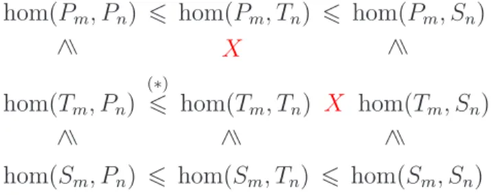
In order to make our paper transparent, we offer the following two tables, Figure 3
and4, which summarize our results. In both tables, the first row follows from Theorem1.2
or its generalization Corollary 3.3. The last row is obvious since hom(Sm, G) is the sum of degree powers of Gand it also follows from Corollary 3.3. The first, second and third columns follow from Theorem 1.4, Theorem 1.5 and Corollary 3.5 respectively. The “X” means that there is no inequality between the two expressions in general and the “?” means that we do not know whether the statement is true or not.
hom(Pm, Pn) 6 hom(Pm, Tn) 6 hom(Pm, Sn)
> X >
hom(Tm, Pn)
(∗)
6 hom(Tm, Tn) X hom(Tm, Sn)
> > >
hom(Sm, Pn) 6 hom(Sm, Tn) 6 hom(Sm, Sn)
Figure 3: The number of homomorphisms between trees of sizesm andn. The (∗) means that there are some well-determined (possible) counterexamples which should be excluded.
hom(Pn, Pn) 6 hom(Pn, Tn) 6 hom(Pn, Sn)
> ? >
hom(Tn, Pn) 6 hom(Tn, Tn) X hom(Tn, Sn)
> > >
hom(Sn, Pn) 6 hom(Sn, Tn) 6 hom(Sn, Sn)
Figure 4: The number of homomorphisms and endomorphisms of trees of size n.
2
The Tree-walk algorithm
In this section we shall state an algorithm for the number of homomorphisms from a tree to any graph. As a generalized concept of walks in graphs, we call a homomorphism from a tree to a graph a tree-walk on this graph.
Let a= (a1, a2, . . . , an) and b = (b1, b2, . . . , bn) be two vectors. We usually denote by
kak = a1 +a2 +· · ·+an the norm of a and by a∗b = (a1b1, . . . , anbn) the Hadamard
product of aand b. Denote by1n then-dimensional row vector with all entries are equal
to 1. Let Gbe a graph with n vertices. The adjacency matrix of G is the n×n matrix
AG := (auv)u,v∈V(G), where auv = 1 when uv ∈ E(G), otherwise 0. We begin with a fundamental lemma about the number of walks in a graph.
Lemma 2.1. Let G be a labeled graph and A=AG the adjacency matrix of G. Then the
(i, j)-entry of the matrix An counts the number of walks in G from vertex i to vertex j
with length n.
Proof. By easy induction on n. See for example [20, Theorem 4.7.1].
Definition 2.2 (hom-vector). LetT be a tree andG be a graph with vertices labeled by 1,2, . . . , n. Let v ∈V(T) be any vertex of T. The n-dimensional vector
h(T, v, G) := (h1, h2, . . . , hn) where
hi =|{f ∈Hom(T, G)| f(v) =i}|,
is called thehom-vector atvfromT toG. Clearly, hom(T, G) =kh(T, v, G)k. Sometimes, we also call h(T, v, G) the hom-vector from the rooted tree T(v) to the graph G and use the more compact notation h(T(v), G).
The following Tree-walk algorithm can be viewed as a generalization of Lemma 2.1for computing the number of tree-walks in graphs.
The Tree-walk algorithm. Let A =AG be the adjacency matrix of the labeled graph
G. Let v be a vertex of the tree T. We now give the algorithm to compute h(T, v, G). We consider two type of recursion steps.
Recursion 1. Ifv is a non-leaf vertex of T, then we can decomposeT toT1∪T2 such that V(T1)∩V(T2) ={v}, and T1 and T2 are strictly smaller than T. In this case
h(T, v, G) = h(T1, v, G)∗h(T2, v, G).
Recursion 2. If v is a leaf with the unique neighbor u inT, then
h(T, v, G) =h(T −v, u, G)A.
Hence we use Recursion 1 or Recursion 2 according to the vertex v is a non-leaf or a leaf. In most of the proofs we simply check whether some property of the vectorh(T, v, G) remains valid after applying Recursion 1 and Recursion 2.
Note that if a leaf has distancedfrom the closest vertex of degree at least 3 then we can execute a sequence of Recursion 2 in one step by simply multiplying the corresponding hom-vector by Ad. This way we can speed up the algorithm a bit. For the sake of convenience, we include an example.
c 6 5 4 3 2 7 1 f d b a e T G
Figure 5: A labeled tree T and a graph G.
Example 2.3. Let T and G be the tree and the graph depicted in Fig. 5. Denote by
T[V] the induced subtree on the vertex set V ⊆V(T). Let us compute h(T,7, G) by the Tree-walk algorithm. First, we compute h(T[1,3],3, G) by using Recursion 2:
h(T[1,3],3, G) = 17AG= (2,3,3,4,1,1). Next we compute h(T[1,2,3],3, G) by using Recursion 1:
h(T[1,2,3],3, G) =h(T[1,3],3, G)∗h(T[2,3],3, G) = (4,9,9,16,1,1).
Now let us compute h(T[1,2,3,4],4, G) by using Recursion 2 again:
h(T[1,2,3,4],4, G) =h(T[1,2,3],3, G)AG= (25,29,26,23,9,16). As a next step we determine h(T[6,5,4],4, G):
h(T[6,5,4],4, G) =17A2G = (7,9,8,9,3,4). Hence h(T[1,2,3,4,5,6],4, G) =h(T[1,2,3,4],4, G)∗h(T[6,5,4],4, G) =(175,261,208,207,27,64). Finally, h(T,7, G) =h(T[1,2,3,4,5,6],4, G)AG= (468,590,495,708,208,207). Thus hom(T, G) =kh(T,7, G)k= 2676.
3
Proof of Theorem
1.3
The main purpose of this section is to prove Theorem 1.3. We shall give an inductive proof of Theorem 1.2 which can be generalized to tree-walks by the tree-walk algorithm. We first need some notations. Let T be a tree and T′ = KC(T, p0, pk) its
KC-transformation with respect to a pathP of length k, a path with vertices labeled consec-utively with p0, p1, . . . , pk. We denote by A and B the components of p0 and pk in the
subgraph of T by deleting all the edges of P. LetA′,B′ and P′ be the components ofT′
corresponding with components A, B and P under the KC-transformation, respectively. The vertices of the path P′ will be labeled consecutively with p′
0, p′1, . . . , p′k, where p′i is corresponding to pi for 06i6k. So p0 ∈A, pk∈ B inT, and p′0 ∈A′, B′ inT′.
Lemma 3.1. Let a1, a2, b1, b2, c1, c2, d1, d2 be positive numbers satisfying the inequalities:
ai > max(ci, di), ai +bi > ci +di for i = 1,2. Then a1a2 > max(c1c2, d1d2) and a1a2 +
b1b2 >c1c2+d1d2.
Proof. Clearly, we only have to prove that a1a2+b1b2 >c1c2+d1d2, the other inequality
is trivial. Note that bi >max(0, ci+di−ai). If one of ci+di−ai <0, say c1+d1 < a1 then
a1a2 >(c1 +d1)a2 >c1c2+d1d2.
If both ci+di−ai >0 fori= 1,2, then
a1a2 +b1b2 >a1a2+ (c1+d1−a1)(c2+d2−a2)
=c1c2+d1d2+ (a1−c1)(a2−d2) + (a1−d1)(a2−c2)>c1c2+d1d2.
Hence we are done.
We first treat the case of k being even.
Proof of first part of Theorem 1.3. In this proofkis even: k = 2t. We labelV(A)\p0with
{am |16m6M},V(A′)\p′0 with{a′i | 16m 6M}, V(B)\pk with{bn |16n 6N} and V(B)\p′
0 with {b′n | 16n 6N}, where am (resp. bn) is corresponding to a′m (resp.
b′
n) under the KC-transformation. Forv ∈H, we always write
h(H, v, T) = (a1, a2, . . . , aM, p0, p1, . . . , pk, b1, b2, . . . , bN) and
h(H, v, T′) = (a′1, a′2, . . . , a′M, p′0, p′1, . . . , p′k, b′1, b′2, . . . , b′N),
where we use the labels of vertices ofT andT′ to index the parameters of the hom-vectors
to T and T′ respectively. We hope that it will not cause any confusion. We shall prove
by induction on the steps of tree-walk algorithm that
a′m >am, b′n >bn
p′i+p′k−i >pi+pk−i
p′i >pi, p′i >pk−i for 16m6M,16n 6N,06i6t.
It is easy to verify that all these inequalities are satisfied after applying any recursion step of the tree-walk algorithm. When v is a leaf of H then it is trivial that these inequalities are preserved. If v is not a leaf then we use Lemma 3.1 to see that the Hadamard-product preserves these inequalities.
Lemma 3.2. Let k be odd and assume that A and B have at least two vertices. Let
am(r), bn(r), pi(r), a′
m(r), b′n(r), p′i(r) denote the number of homomorphism of Pr into T
and T′, respectively, such that the endvertex of P
r goes to the vertices am, bn, pi, a′m, b′n
and p′
i, respectively. Then the following inequalities hold for every r:
a′m(r)>am(r), b′n(r)>bn(r) (3.1)
p′i(r) +p′j(r)>pi(r) +pj(r) (3.2)
p′i(r) +p′j(r)>pk−i(r) +pk−j(r) (3.3)
for 16m6M,16n 6N and i+j 6k.
Proof. We prove the claim by induction on r. For r= 1,2, the claim is trivial. Note that
we only have to prove that
a′
m(r)>am(r), b′n(r)>bn(r)
p′i(r) +p′j(r)>pi(r) +pj(r)
for 16m6M,16n 6N and i+j 6k. We obtain the inequality
p′i(r) +p′j(r)>pk−i(r) +pk−j(r)
by simply exchanging the role of A and B. Also note that if we put i = j in the inequality (3.2) and (3.3) we obtain that p′
i(r)>pi(r), pk−i(r) fori < k/2.
Observe that for any vertex v we have:
v(r) = X u∈N(v)
u(r−1).
We will treat the cases k = 1 andk >3 separately.
Case 1: k = 1. In this case, we have to prove the inequalities:
a′m(r)>am(r), b′n(r)>bn(r), p′0(r)>max(p0(r), p1(r)), p′0(r) +p′1(r)>p0(r) +p1(r).
The inequalities a′
m(r) > am(r), b′n(r) > bn(r) simply follow from the inequalities
a′ m(r−1)>am(r−1), b′n(r−1)>bn(r−1), and p′0(r−1)>p0(r−1), p1(r−1). Observe that p′0(r) = X a′ m∈N(p′0) a′m(r−1) + X b′ n∈N(p′0) b′n(r−1) +p′1(r−1) = X a′ m∈N(p′0) a′m(r−1) + X b′ n∈N(p′0) b′n(r−1) +p′0(r−2) > X am∈N(p0) am(r−1) + X bn∈N(p1) bn(r−1) +p0(r−2) > X am∈N(p0) am(r−1) + X bn∈N(p1) bn(r−2) +p0(r−2)
= X am∈N(p0)
am(r−1) +p1(r−1) = p0(r).
We used the induction hypothesis and that bm(r−1) > bm(r−2). In general, u(r) >
u(r−1) since any homomorphism of Pr−1 starting at the vertex u can be extended to a
homomorphism ofPr starting atu. Clearly, we can getp′0(r)>p1(r) similarly, or we just
switch the role of A and B. Finally, p′0(r) +p′1(r) = X a′ m∈N(p′0) a′m(r−1) + X b′ n∈N(p′0) b′n(r−1) +p′0(r−1) +p′1(r−1) > X am∈N(p0) am(r−1) + X bn∈N(p1) bn(r−1) +p0(r−1) +p1(r−1) =p0(r) +p1(r).
Hence we are done in this case.
Case 2: k > 3. Clearly, the inequalities a′
m(r) > am(r), b′n(r) > bn(r) simply follow from the inequalities a′
m(r −1) > am(r −1), b′n(r−1) > bn(r −1), and p′0(r −1) > p0(r−1), pk(r−1) as before.
So we only have to prove the inequality p′
i(r) +p′j(r)>pi(r) +pj(r) fori+j 6k. We can assume that i6j. If i>1, then j 6k−1 and
p′i(r) +p′j(r) = (p′i−1(r−1) +pj′+1(r−1)) + (p′i+1(r−1) +p′j−1(r−1))
>(pi−1(r−1) +pj+1(r−1)) + (pi+1(r−1) +pj−1(r−1))
=pi(r) +pj(r).
So we only have to consider the case i = 0. In this case we consider the cases j = 0, j = 1,26j 6k−2, j =k−1, j =k separately. Unfortunately, all of them behaves a bit differently. Subcase j = 0: 2p′0(r) = 2 X a′ m∈N(p′0) a′m(r−1) + X b′ n∈N(p′0) b′n(r−1) +p′1(r−1) >2 X am∈N(p0) am(r−1) +p1(r−1) = 2p0(r), since p′ 1(r−1)>p1(r−1), because 1< k/2. Subcase j = 1: p′0(r) +p′1(r) = X a′ m∈N(p′0) a′m(r−1) + X b′ n∈N(p′0) b′n(r−1) +p′1(r−1) +p′0(r−1) +p′2(r−1)
> X
am∈N(p0)
am(r−1) +p1(r−1) +p0(r−1) +p2(r−1) =p0(r) +p1(r),
since p′
1(r−1)>p1(r−1) andp′0(r−1) +p′2(r−1)>p0(r−1) +p2(r−1).
Subcase 2 6j 6k−2: Here we jump back fromr tor−2, so we need a few notations.
LetdA and dB denote the degree of p0′ in A and B, respectively. Furthermore, let d(v, u)
denote the distance of the vertices u and v. Then
p′0(r) +p′j(r) = X a′ m:d(a′m,p′0)=2 a′m(r−2) + X b′ n:d(b′n,p′0)=2 b′n(r−2) + (dA+dB+ 1)p′0(r−2) +p′2(r−2) +p′j−2(r−2) + 2p′j(r−2) +p′j+2(r−2)> > X am:d(am,p0)=2 am(r−2) + (dA+ 1)p0(r−2) +p2(r−2)+ +pj−2(r−2) + 2pj(r−2) +pj+2(r−2) = p0(r) +pj(r), since the inequality follows from the following inequalities:
a′m(r−2)>am(r−2) b′n(r−2)>0 (dB−1)p′0(r−2)>−p0(r−2) (dA−1)p′0(r−2)>(dA−1)p0(r−2) p′2(r−2) +p′j−2(r−2)>p2(r−2) +pj−2(r−2) 2(p′0(r−2) +p′j(r−2))>2(p0(r−2) +pj(r−2)) p′0(r−2) +p′j+2(r−2)>p0(r−2) +pj+2(r−2). Subcase j = k−1: p′0(r) +p′k−1(r) = X a′ m∈N(p′0) a′m(r−1) + X b′ n∈N(p′0) b′n(r−1) +p′1(r−1) +p′k−2(r−1) +p′k(r−1) = X am:d(a′m,p′0)=2 a′m(r−2) +dAp′0(r−2) + X b′ n∈N(p′0) b′n(r−1) +p0′(r−2) +p′2(r−2) +p′k−3(r−2) + 2p′k−1(r−2).
On the other hand,
p0(r) +pk−1(r)
= X
am∈N(p0)
= X am:d(am,p0)=2 am(r−2) +dAp0(r−2) +p0(r−2) +p2(r−2) +pk−3(r−2) + 2pk−1(r−2) + X bn∈N(pk) bn(r−2). The inequality p′ 0(r) +p′k−1(r)>p0(r) +pk−1(r) follows from a′m(r−2)>am(r−2) b′n(r−1)>bn(r−1)>bn(r−2) (dA−1)p′0(r−2)>(dA−1)p0(r−2) p′2(r−2) +p′k−3(r−2)>p2(r−2) +pk−3(r−2) 2(p′0(r−2) +p′k−1(r−2)) >2(p0(r−2) +pk−1(r−2)). Subcase j = k: p′0(r) +p′k(r) = X a′ m∈N(p′0) a′m(r−1) + X b′ n∈N(p′0) b′n(r−1) +p′1(r−1) +p′k−1(r−1) > X am∈N(p0) am(r−1) + X bn∈N(pk) bn(r−1) +p1(r−1) +pk−1(r−1) =p0(r) +pk(r).
Proof of the second part of Theorem 1.3. From Lemma 3.2 we only keep the inequalities
a′ m(r)>am(r) b′n(r)>bn(r) p′i(r)>pi(r), pk−i(r) p′i(r) +p′k−i(r)>pi(r) +pk−i(r) for 16 m6M,16n 6N,06i6k/2.
For a tree H and v ∈H, let us write
h(H, v, T) = (a1, a2, . . . , aM, p0, p1, . . . , pk, b1, b2, . . . , bN) and
h(H, v, T′) = (a′1, a′2, . . . , a′M, p′0, p′1, . . . , p′k, b′1, b′2, . . . , b′N),
where we use the labels of vertices ofT andT′ to index the parameters of the hom-vectors
toT andT′, respectively. We say thath(H, v, T)6h(H, v, T′) if the following inequalities
hold
a′m >am
b′
p′i+p′k−i >pi+pk−i
p′i >pi
p′i >pk−i
for 1 6 m 6 M,1 6 n 6 N,0 6 i 6 k/2. As we have seen these inequalities hold for a path Pr and its endvertex. Since these inequalities are preserved for Hadamard-product by Lemma 3.1, we see that h(H, v, T) 6 h(H, v, T′) for starlike trees H, where v is the
center of the starlike tree. This implies that
hom(H, T′)>hom(H, T).
The following generalization of inequality (1.2) follows immediately from Proposi-tion 1.1 and Theorem 1.3.
Corollary 3.3. Let H be a starlike tree and let Tn be a tree on n vertices. Then hom(H, Pn)6hom(H, Tn)6hom(H, Sn).
The reader may wonder that if inequality (1.4) holds when k is odd and H is not a starlike tree. This is not true in general. A counterexample will be constructed in the following, which also shows that
hom(H, Tn)6hom(H, Sn) is not true for any tree H.
Proposition 3.4. Let T be a tree with color classes A and B considered as a bipartite graph. Then
hom(T, Sn) = (n−1)|A|+ (n−1)|B|.
Corollary 3.5. Let Tm be a tree on m vertices, then
hom(Pm, Sn)6hom(Tm, Sn)6hom(Sm, Sn).
If T 6=Sm then the second inequality is strict.
Proof of Proposition 3.4. SinceT and Sn are bipartite graphs, a color class of T have to
go into a color class of Sn. If the color class A goes to the center of Sn, then any vertex belonging to the color class of B can go to any leaf of the star, so it provides (n−1)|B|
homomorphisms. The other case provides (n−1)|A| homomorphisms.
This simple proposition also shows us how to construct a tree Tn for which
hom(Tn, Tn)>hom(Tn, Sn).
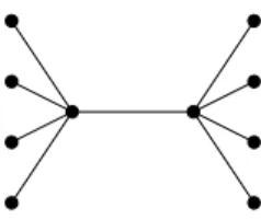
Let Tn = S2∗k be the doublestar on 2k vertices with 2k−2 leaves and two vertices of degree k. Then it is easy to see that
Figure 6: The doublestar S∗ 10.
while
hom(S2∗k, S2k) = 2(2k−1)k.
Hence for k >5 we have
hom(S2∗k, S2∗k)>hom(S2∗k, S2k). Note thatS2k can be obtained from S2∗k by a KC-transformation.
4
Graph homomorphisms from trees
4.1
Markov chains and homomorphisms
Theorem 4.1. Let G be a graph and let P = (pij) be a Markov chain on G:
X
j∈N(i)
pij = 1 for all i∈V(G),
where pij >0 and pij = 0 if (i, j)∈/ E(G). Let Q= (qi) be the stationary distribution of
P:
X
j∈N(i)
qjpji =qi for all i∈V(G).
Let us define the following entropies:
H(Q) = X i∈V(G) qilog 1 qi , and H(D|Q) = X i∈V(G) qilogdi,
where di is the degree of the vertex i, and let
H(P|Q) = X i∈V(G) qi X j∈N(i) pijlog 1 pij .
Let Tm be a tree with ℓ leaves on m vertices, where m>3. Then
hom(Tm, G)>exp
H(Q) +ℓH(D|Q) + (m−1−ℓ)H(P|Q)
.
Proof. Letv be a root of T. Let ai be the number of homomorphisms of Tm into G such that the root vertex v goes into the vertex i∈V(G). Let
F(Tm(v), G) = n Y i=1 aqi i .
We will show by induction on m that
F(Tm(v), G)>exp (ℓ∗H(D|Q) + (m−1−ℓ∗)H(P|Q)),
where ℓ∗ is the number of leaves different from v, so it is ℓ if v is not a leaf andℓ−1 ifv
is a leaf. Note that
F(K2(v), G) = expH(D|Q).
If v is not a leaf of Tm, then we can decompose Tm toT1(v) andT2(v). Then F(Tm(v), G) =F(T1(v), G)F(T2(v), G)
because of the Hadamard-products of the hom-vectors. From this the claim follows im-mediately by induction.
If v is a leaf of Tm with the unique neighbor u, then let
h(Tm−v, u, G) = (b1, . . . , bn). So ai =Pj∈N(i)bj.
For positive numbers r1, . . . , rt and positive weights w1, . . . , wt with Pti=1wi = 1, the weighted AM-GM inequality says that
r1+· · ·+rt=w1 r1 w1 +· · ·+wt rt wt > r1 w1 w1 . . . rt wt wt = exp t X i=1 wilog 1 wi ! t Y i=1 rwi i . Hence F(Tm(v), G) = n Y i=1 aqi i = n Y i=1 X j∈N(i) bj qi > n Y i=1 Y j∈N(i) bj pij pij qi = n Y i=1 Y j∈N(i) 1 pij pijqi n Y i=1 b P j∈N(i)pjiqj i
= n Y i=1 Y j∈N(i) 1 pij pijqi n Y i=1 bqi i .
In the last step we used that Qis a stationary distribution with respect to P. Hence
F(Tm(v), G)>exp(H(P|Q))F((Tm−v)(u), G). Now the claim follows by induction.
To finish the proof of the theorem, we only have to choose a nonleaf root and use that
hom(Tm, G) = n
X
i=1
ai >exp(H(Q))F(Tm(v), G).
Remark 4.2. Note that the inequality H(D|Q)>H(P|Q) always holds. Consequently,
hom(Tm, G)>exp(H(Q) + (m−1)H(P|Q)).
As Theorem 4.1 suggests, this is an inequality for entropies and indeed, it can be proved in this way. By P and Q, we defined a distribution on the set of homomorphisms: we choose a root according to Q, then we choose every nonleaf new vertex according to P
and finally we choose the leaves uniformly. The entropy of this distribution is exactly
H(Q) +ℓH(D|Q) + (m−1−ℓ)H(P|Q) since every nonleaf vertex has distribution Q. Note that this entropy is smaller than the entropy of the uniform distribution, that is, log hom(Tm, G). For basic facts about entropy, see for example [5].
Theorem 4.3. Let Gbe a connected graph on the vertex set{1,2, . . . , n}and let λ be the
largest eigenvalue of the adjacency matrix of the graph G. Let y be a positive eigenvector
of unit length corresponding to λ. Let qi =yi2. Then for any rooted tree Tm on m vertices
we have hom(Tm, G)>exp(Hλ(G))λm−1, where Hλ(G) = n X i=1 qilog 1 qi
is the spectral entropy of the graph G.
Proof. We will use Theorem 4.1. Let pij = λyyji. Since y is a positive eigenvector, we have
pij >0. For all iwe have λyi =Pj∈N(i)yj, thus Pj∈N(i)pij = 1. Forqi =yi2 we have
qipij =y2i yj λyi = 1 λyiyj =qjpji. Hence X i∈N(j) qjpji= X i∈N(j) qipij =qi.
This means that P = (pij) is a Markov chain with stationary distributionQ = (qi). The conditional entropy H(P|Q) = X i∈V(G) qi X j∈N(i) pijlog 1 pij = X i∈V(G) y2 i X j∈N(i) yj λyi logλyi yj = X {i,j}∈E(G) yiyj λ 2 logλ+ log yi yj + log yj yi = log(λ)1 λ X (i,j)∈E(G) yiyj = logλ.
Hence the result follows from Theorem 4.1.
Remark 4.4. A Markov chain is called reversible if qipij =qjpji for all i, j ∈ V(G). As we have seen, the Markov chain constructed in the previous proof is reversible. It is not hard to show that on trees every Markov chain is reversible.
Remark 4.5. Theorem 4.3 is the best possible in the sense that there cannot be a larger number than λ in such a statement since
hom(Pm, G)6nλm−1. Indeed, hom(Pm, G) n = 1nTAm−11n 1nT1n 6max v6=0 vTAm−1v vTv =λmax(A m−1) =λm−1.
Note that we can deduce that if (Tm)∞
m=1 is a sequence of trees such that Tm has m vertices then lim inf m→∞ hom(Tm, G) 1/m>lim inf m→∞ hom(Pm, G) 1/m=λ.
This result could have been deduced as well from a theorem of B. Rossman and E. Vee [21] claiming that
hom(Tm, G)>hom(Cm, G),
whereCm is the cycle on mvertices. In fact, this was proved for directed trees and cycles, but it implies the inequality for undirected tree and cycle. This result can also be deduced from Theorem 3.1 of [13].
The following special case of Theorem 4.1, involving the degree sequence of graphs, is Theorem 3 in the paper [9].
Theorem 4.6 (Dellamonica et al.). Let G be a graph on the vertex set {1,2, . . . , n} with
e(G) edges and with degree sequence(d1, . . . , dn). Then for any tree Tm on m vertices we
have hom(Tm, G)>2e(G)·Cm−2, where C = n Y i=1 ddi i !1/2e(G) .
Proof. Let us consider the following classical Markov chain: pij = d1i if j ∈ N(i). The
stationary distribution is qi = 2ed(iG). Note that
H(P|Q) = X i∈V(G) qi X j∈N(i) pijlog 1 pij = X i∈V(G) qilogdi = 1 2e(G) X i∈V(G) dilogdi = logC and H(Q) +H(P|Q) = X (i,j)∈E(G) qipijlog 1 qipij = X (i,j)∈E(G) 1 2e(G)log(2e(G)) = log(2e(G)). Hence the result follows from Theorem 4.1.
Definition 4.7. The homomorphism density t(H, G) is defined as follows:
t(H, G) = hom(H, G)
|V(G)||V(H)|.
This is the probability that a random map is a homomorphism. Sidorenko’s conjecture says that
t(H, G)>t(K2, G)e(H)
for every bipartite graph H withe(H) edges. It is known that Sidorenko’s conjecture [18] is true for trees. By now, there are many proofs for this particular case of Sidorenko’s conjecture: see [11,15] and it can be deduced as well from Theorem 3.1 of [13]. Below we give a new proof for this fact.
Theorem 4.8. For any tree Tm on m vertices and a graph G we have
t(Tm, G)>t(K2, G)m−1.
Proof. Let |V(G)| = n. The theorem will immediately follows form Theorem 4.6. By
convexity of the function xlogxwe have 1 2e(G) X i∈V(G) dilogdi > 1 2e(G)n 2e(G) n log 2e(G) n = log2e(G) n . Hence t(Tm, G) = hom(Tm, G) nm > 1 nm2e(G) 2e(G) n m−2 = 2e(G) n2 m−1 =t(K2, G)m−1.
4.2
Sidorenko’s theorem on extremality of stars
The objective of this section is to give a new proof for Theorem 1.5 in order to keep this paper self-contained. This was proved originally by Sidorenko [19]. Our proof is very similar to the original one, but it is slightly more elementary.
Before we start the proof we will need two definitions and two lemmas.
Definition 4.9. LetMu and Nv be two rooted graphs with root vertices uand v, respec-tively. Then Mu ◦u=v Nv denotes the graph obtained from Mu ∪Nv by identifying the vertices uand v.
Lemma 4.10. Let Ru,v be a graph with specified (not necessarily distinct) vertices u and
v. Let Ju′ and Kv′ be two graphs with root verticesu′ and v′. Finally, let the graphs A, B
and C be obtained from Ru,v, Ju′, Kv′ as follows:
A= (Ru,v◦u=u′ Ju′)◦v=v′ Kv′,
B = (Ru,v◦u=u′ Ju′)◦u=u′ Ju′,
C = (Ru,v◦v=v′ Kv′)◦v=v′ Kv′.
(In other words, in B and C we attach two copies of the same graph at the specified
vertex.) Then for any graph G we have
2 hom(A, G)6hom(B, G) + hom(C, G).
Proof. Leti, j ∈V(G) and let h(Ru,v, i, j) denote the number of homomorphisms ofRu,v
toG where u goes to iand v goes to j. We similarly define h(Ju′, i) andh(Kv′, j). Then
hom(A, G) = X i,j∈V(G) h(Ru,v, i, j)h(Ju′, i)h(Kv′, j). Similarly, hom(B, G) = X i,j∈V(G) h(Ru,v, i, j)h(Ju′, i)2, and hom(C, G) = X i,j∈V(G) h(Ru,v, i, j)h(Kv′, j)2. Hence
hom(B, G) + hom(C, G)−2 hom(A, G)
= X
i,j∈V(G)
h(Ru,v, i, j)(h(Ju′, i)−h(Kv′, j))2 >0.
Definition 4.11. Let d(u, v) be the distance of the vertices u, v ∈ V(G). Then the
Wiener-index W(G) of a graph Gis defined as
W(G) := X u,v∈V(G)
d(u, v).
In our application Ru,v will be a tree and Ju′ and Kv′ be the trees on 2 vertices. The following lemma about the Wiener-index is trivial.
Lemma 4.12. Let Ru,v be a tree with distinct vertices u and v. Let Ju′ and Kv′ be
two copies of the two-node trees with root vertices u′ and v′, respectively. Finally, let
the graphs A, B and C be obtained from Ru,v, Ju′, Kv′ as in the former lemma. Then
2W(A)> W(B) +W(C).
Proof of Theorem 1.5. Let TG be the set of those trees F on m vertices for which
hom(F, G) is maximal. Let T ∈ TG be the tree for which W(T) is minimal. We show that T = Sm. Assume for contradiction that T 6= Sm. Then T has two leaves, a and b
such that d(a, b)>3. Let uand v be the unique neighbors ofa and b, respectively. Then
u6=v. Let Ru,v =T − {a, b}, Ju′ ={u′, a}and Kv′ ={v′, b}. Then
A = (Ru,v ◦u=u′ Ju′)◦v=v′ Kv′ =T. As in the lemmas, let
B = (Ru,v◦u=u′ Ju′)◦u=u′ Ju′,
C = (Ru,v◦v=v′ Kv′)◦v=v′ Kv′.
Note thatB and C are also trees on m vertices. By the Lemma we have 2 hom(A, G)6hom(B, G) + hom(C, G).
Since A = T ∈ TG, then hom(B, G) + hom(C, G) 6 2 hom(A, G). So hom(A, G) = hom(B, G) = hom(C, G) implying that B, C ∈ TG as well. But then 2W(T)> W(B) +
W(C), so one of them has strictly smaller Wiener-index than T, this contradicts the choice of T. Hence T must be Sm.
Remark 4.13. Let E7 be the tree obtained from P6 by putting a pendant edge to the third vertex of the path. Then there is a tree T for which
hom(P7, T)>hom(E7, T).
The following tree T is suitable: letT =T(k1, k2, k3) be the tree where the root vertex v0
havek1 neighbors, all of its neighbors hask2+1 neighbors and the vertices having distance 2 from v0 have k3+ 1 neighbors. If we choose k1, k2, k3 such that k2 ≪k1 ≪k3 ≪ k1k2
(for instance ki =kαi, where α2 < α1 < α3 < α1 +α2 and k is large), then
5
Proofs of Theorems
1.6
and
1.8
In this section we give the proof of Theorem 1.6 and Theorem 1.8. As we will see, Theorem 1.6 with some additional observations implies Theorem 1.8.
To prove Theorem 1.6 we will build on the fact that there are not many homomor-phisms into a path. Indeed, by Theorem 1.5 we have
hom(Tm, Pn)6hom(Sm, Pn) = (n−2)2m−1+ 2.
So for a particular tree Tn, it is enough to prove that for every treeTm we have
hom(Tm, Tn)>(n−2)2m−1+ 2. (5.1)
This would immediately imply that
hom(Tm, Tn)>hom(Tm, Pn). (5.2)
We will prove that inequality 5.1 is indeed true for all trees Tn with at least four leaves and for a large class of trees with three leaves. For the remaining trees with three leaves we use Theorem 1.3.
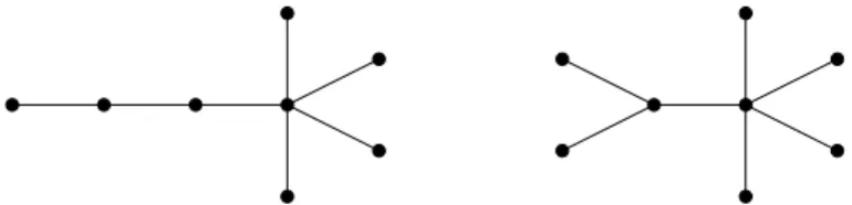
Figure 7: The trees T8 (left) and T′
8 (right).
Remark 5.1. To prove Theorem 1.6 and Theorem 1.8 we cannot rely entirely on the use of KC-transformation. That is why we had to find another strategy to prove these theorems.
Indeed, KC-transformation does not always increase the number of endomorphisms of trees. The first counterexample is the two trees on 8 vertices in Fig.7. The tree T′
8 is the
KC-transformation ofT8, but |End(T′
8)|= 10430<17190 = |End(T8)|.
5.1
The extremality of the star
Note that Theorem 1.5 and Theorem 1.3 together implies the following chain of inequal-ities:
|End(Tn)|= hom(Tn, Tn)6hom(Sn, Tn)6hom(Sn, Sn) =|End(Sn)|, since Sn is a starlike tree. In this section, we will also give a direct proof for it.
Theorem 1.8(Second part). Let Tn be a tree on n vertices. Then
|End(Tn)|6|End(Sn)|.
Proof. For the sake of simplicity we prove the statement for n > 17. The same proof applies to n < 17, we only need to compute a bit more carefully. In the end of the proof we will give the details of this more precise calculation.
Note that |End(Sn)|= (n−1)n−1+ (n−1).
Let Tn be a tree onn vertices and let d =d1 > d2 >. . .>dn be its degree sequence. Note that d1+d2 6n, since the tree has onlyn−1 edges and the stars corresponding to the first two largest degrees can share at most one common edge.
First we prove that |End(Tn)| 6ndn−1. To see it, let u1, . . . u
n be the vertices of the tree Tn such that u1, . . . , uk induces a tree for every k. Then we can chose the image of
u1 by n ways, and if we have already chosen the image ofu1, . . . , uk−1, then we can chose
the image of uk in at mostd ways, since it must be the neighbor of some previous vertex. This means that |End(Tn)|6ndn−1.
If d62n/3 then ndn−1 6n 2n 3 n 6(n−1)n−1 if n >17, since then 3 2 n >en2 >n2 1 + 1 n−1 n−1 .
So we can assume that d > 23n. Set d = n −k. We can assume that Tn 6= Sn, consequently k > 2. Let v1 be the vertex having the largest degree and v2, . . . , vd+1 its
neighbors. Now we can decompose the set of endomorphisms according to the image ofv1
is v1 or not. If it is v1 then there can be at most dn−1 such endomorphisms. If the image
of v1 is not v1, then we can chose that image in at most (n−1) ways and the image of v2, v3, . . . , vd+1 can be chosen at most d2 times and the image of all other vertices can be
chosen in at most d ways. Hence
|End(Tn)|6dn−1+ (n−1)dd2dn−1−d.
All we need to prove is that if d6n−2 then
dn−1+ (n−1)dd2dn−1−d6(n−1)n−1+ (n−1).
With the notations d=n−k we have
dn−1+ (n−1)d2ddn−1−d6(n−k)n−1+ (n−1)kn−k(n−k)k−1.
By the binomial theorem we have
(n−1)n−1 = (n−k+k−1)n−1 >(n−k)n−1+ (n−1)(n−k)n−2(k−1).
It is enough to prove that (n−k)n−2 >kn−k(n−k)k−1. This is equivalent with
and it is true since it is equivalent with
n k −1
n−k
>2n−k>n−k.
In the last step we have used that n/k >3.
It is clear from the proof that we only have to check whether one of the inequalities hold for some d:
n 6 n−1 d n−1 or n k −1 n−k >n−k.
For 8 6 n 6 16 it is easy to see that if d 6 n−4 then the first inequality holds and if
d > n−4, equivalently k 6 3 then the second inequality holds. For n = 5,6,7 the first
inequality holds if d 6 n−3, and the second inequality holds if d > n−3, equivalently
k 62. For n= 4 the claim is trivial 30 =|End(S4)|>|End(P4)|= 16.
5.2
The extremality of the path
Theorem 5.2. Let Tm and Tn be trees on m and n vertices, respectively. If the tree Tn
has at least four leaves, then
hom(Tm, Tn)>(n−2)2m−1+ 2. An easy consequence of this theorem is the following.
Corollary 5.3. If Tn is a tree on n vertices with at least 4 leaves, then hom(Tm, Tn)>hom(Tm, Pn).
Proof. Indeed,
hom(Tm, Tn)>(n−2)2m−1 + 2 = hom(Sm, Pn)>hom(Tm, Pn), where the second inequality follows from Theorem 1.5.
A consequence of this theorem and Theorem 1.4 (the proof of which will be given in the follow-up paper [8]) is that path has the minimal number of endomorphisms.
Theorem 1.8(First part). For all trees Tn onn vertices we have
|End(Tn)|>|End(Pn)|.
Proof. If Tn has at least four leaves, then
hom(Tn, Tn)>hom(Tn, Pn)>hom(Pn, Pn),
where the first inequality follows from Corollary 5.3, while the second inequality follows from Theorem 1.4. If the tree Tn has exactly three leaves, then it is star-like. Hence we can use Theorem 1.3 to prove the first inequality:
The proof of Theorem 5.2 will be given next, which would complete the proof of Theorem 1.8.
First, we prove a reduction lemma which says that we only have to prove Theorem 5.2
for trees with exactly 4 leaves.
Lemma 5.4 (Reduction lemma). Let Tm be a tree on m vertices and let n be fixed.
Assume that for any tree Tk we have
hom(Tm, Tk)>(k−2)2m−1+ 2,
where k < n and Tk has at least four leaves, or k = n and Tk has exactly four leaves.
Then for any tree Tn on n vertices with at least 4 leaves we have
hom(Tm, Tn)>(n−2)2m−1+ 2.
In the proof of this lemma we will subsequently use the following very simple fact.
Fact. IfG is a graph and G1, G2 are induced subgraphs of G with possible intersection, then for any graph H we have
hom(H, G)>hom(H, G1) + hom(H, G2)−hom(H, G1∩G2).
Proof of the lemma. We can assume that m> 2. Assume that Tn is a tree with at least
5 leaves. Otherwise we have nothing to prove.
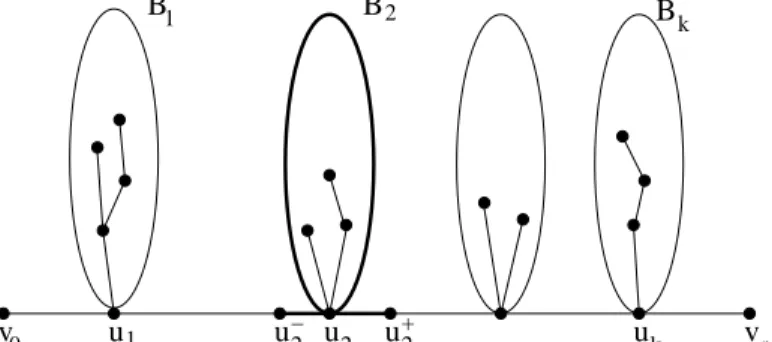
Let us call a path maximal in Tn if it connects leaves. If a maximal path contains k vertices of degree at least 3, then we say that the maximal path has k branches.
Case 1: Tn contains a maximal path with at least 3 branches. Let v0P vr be a maximal path with vertices u1, . . . , uk having degree at least 3. Let B1, . . . , Bk be the branches which we get if we delete all vertices and edges of the path v0P vr except
u1, . . . , uk. So Bi is a rooted tree with rootui. Let u−2 and u+2 be the two neighbors of u2
on the path v0P vr. Let T(2) be the tree induced by the vertices V(B2)∪ {u−
2, u+2}. Let
|V(T(2))|=t. We distinguish two cases.
v0 u1 u2− u2 u2+ u vr
B1 B2 Bk
k
Subcase 1.1: hom(Tm, T(2)) < (t−2)2 m−1
+ 2. Consider the following treesG1 and
G2. G1 is the tree spanned by the vertices v0P u+2 and the branches B1, B2. G2 is the tree spanned by the vertices u−2P vr and the branches B2, . . . , Bk. Note that G1 ∪G2 = Tn,
G1∩G2 =T(2) and G1, G2 contains at least 4 leaves, because k >3. By the hypothesis
of the lemma we have
hom(Tm, Gi)>(|V(Gi)| −2)2m−1+ 2 for i= 1,2. Hence
hom(Tm, Tn)>hom(Tm, G1) + hom(Tm, G2)−hom(Tm, G1∩G2)>
>(|V(G1)| −2)2m−1+ 2 + (|V(G2)| −2)2m−1+ 2−((|V(G1∩G2)| −2)2m−1+ 2) = = ((|V(G1∪G2)| −2)2m−1+ 2 = (n−2)2m−1+ 2.
In this case we are done.
Case 1.2: hom(Tm, T
(2))> (t
−2)2
m−1
+ 2. Consider the following treesG1 and G2.
G1 is the tree spanned by the vertices (V(Tn)\V(T(2)))∪ {u−
2, u2, u+2}. G2 is simply T(2).
Note that G1∪G2 =Tn, G1 ∩G2 ={u−2, u2, u+2}=P3 and G1 contains at least 4 leaves.
By the hypothesis of the lemma we have
hom(Tm, G1)>(|V(G1)| −2)2m−1 + 2.
We also know that in this case
hom(Tm, G2)>(|V(G2)| −2)2m−1 + 2.
Note that
hom(Tm, P3)6hom(Sm, P3) = 2m−1+ 2.
Then
hom(Tm, Tn)>hom(Tm, G1) + hom(Tm, G2)−hom(Tm, G1∩G2)>
>(|V(G1)| −2)2m−1+ 2 + (|V(G2)| −2)2m−1+ 2−((|V(G1∩G2)| −2)2m−1+ 2) = = ((|V(G1∪G2)| −2)2m−1+ 2 = (n−2)2m−1+ 2.
In this case we are done too.
Case 2: All maximal paths of Tn have at most 2 branches. In the following we show that they have quite simple structure: they are starlike or double starlike trees, see Figure 9.
Let v1 be a vertex of Tn of degree at least 3. Let us decompose Tn to the branches
B′
1, B2′, . . . Bk′ at v1. So v1 is a leaf in the trees B1′, B2′, . . . Bk′. We show that all except at most one ofB′
1, B2′, . . . , B′k are paths. Assume that, for instance, B1′, B2′ are not paths.
Then they contains at least two leaves ofTn: B′
1 containsu1, u2,B2′ containsu3, u4. Then
the maximal pathu1P u3 has at least three branches: one-one inside the branchesB′
1 and
B′
v v a a a b b 1 2 s 1 2 b bt 3 1 2
Figure 9: A double starlike tree.
one of them is not path, sayB′
1, then let us consider the vertexv2 ∈V(B′1) having degree
at least 3 which is closest to v1. Repeating the previous argument to v2 instead of v1, all except one branches at v2 must be path and we also know that the branch containing v1
is not path. Hence the tree is double starlike, where the middle path is v1P v2.
We can consider a starlike tree as a double starlike tree, where v1 =v2. Let a1, . . . , as and b1, . . . , bt be the leaves of Tn, where a1, . . . , as are closer to v1 than to v2, while
b1, . . . , bt are closer to v2 than to v1. If v1 =v2 we just decompose the set of leaves into two sets of (almost) equal size. Note thats, t>2. Since we can assume that there are at least 5 leaves, we assume thats+t >5.
Ifu1, . . . , uℓ are some vertices of a tree, then we say that the tree spanned byu1, . . . , uℓ is the smallest subtree which contains the vertices u1, . . . , uℓ. It is
span(u1, . . . , uℓ) =∪16i,j6ℓuiP uj.
Subcase 2.1: If s >3 and t > 3 both hold, then let G1 be the tree spanned by the vertices a1, a2, b1, b2, and let G2 be the tree spanned by the vertices a2, . . . as, b2, . . . , bt. Then G1∪G2 =Tn, G1∩G2 =a2P b2 and bothG1, G2 have at least 4 leaves. Since
hom(Tm, G1∩G2)6hom(Sm, G1∩G2) =
= hom(Sm, a2P b2) = (|V(G1∩G2)| −2)2m−1+ 2, we have
hom(Tm, Tn)>hom(Tm, G1) + hom(Tm, G2)−hom(Tm, G1∩G2)>
>(|V(G1)| −2)2m−1+ 2 + (|V(G2)| −2)2m−1+ 2−((|V(G1∩G2)| −2)2m−1+ 2) = = (|V(G1∪G2)| −2)2m−1+ 2 = (n−2)2m−1+ 2.
Hence we are done in this case.
Subcase 2.2: Ifs >4 andt = 2 then let G1 be the tree spanned by a1, a2, b1, b2 and let G2 be the tree spanned by a2, . . . , ak, b1. Then G1 ∪G2 = Tn, G1∩G2 = a2P b1 and both G1, G2 have at least 4 leaves. In this case we are done as before. Clearly, the case
Subcase 2.3: The last case is s = 3, t = 2 (and s = 2, t = 3). Let G1 =
span(a1, a2, b1, b2), G2 = span(a2, a3, b1, b2), G3 = span(a2, b1, b2), G4 = (a1, a2, a3, v2). Then G1∩G2 =G3, G3∩G4 =a2P v2. Note that G1, G2, G4 has 4 leaves, thus
hom(Tm, Gi)>(|V(Gi)| −2)2m−1+ 2
fori= 1,2,4. If hom(Tm, G3)6(|V(G3)|−2)2m−1+2, then fromTn =G1∪G2,G3 =G1∩
G2we obtain that hom(Tm, Tn)>(n−2)2m−1+2. If hom(Tm, G3)>(|V(G3)|−2)2m−1+2, then from Tn =G3 ∩G4 we obtain that hom(Tm, Tn) > (n−2)2m−1+ 2. Hence we are done in this case as well.
Proof of Theorem 5.2. The result immediately follows from Lemma 5.4 and Proposi-tion 5.5 below.
Proposition 5.5. Let Tn be a tree on n vertices with exactly four leaves. Then for any
tree Tm on m vertices we have
hom(Tm, Tn)>(n−2)2m−1+ 2,
where n is the number of vertices of Tn.
Proof. If Tn has a vertex of degree 4 then by Theorem 4.6 we have
hom(Tm, Tn)>2(n−1)Cm−2, where C = n Y i=1 ddi i !1/2e(Tn) = 2. Hence hom(Tm, Tn)>(n−1)2m−1 >(n−2)2m−1+ 2.
For the case when Tn has two vertices of degree 3, we need more preparation.
Lemma 5.6. Let Tn be a tree with exactly 4 leaves and two vertices of degree 3. Let x
and y be the vertices of Tn with degree 3. Assume that there are at most 3 vertices of Tn
which have degree 2 and not on the path xP y. Then for any tree Tm on m vertices we
have
hom(Tm, Tn)>(n−2)2m−1+ 2,
where n is the number of vertices of Tn.
Proof. We can assume that m > 4, otherwise the statement is trivial. We prove the
slightly stronger inequality
hom(Tm, Tn)> n−2 + 1 8 2m−1.
If m>4, then this implies that
hom(Tm, Tn)>(n−2)2m−1+ 1 or equivalently,
hom(Tm, Tn)>(n−2)2m−1+ 2.
To prove this statement we use Theorem 4.1 with a suitable Markov chain. Let pij = 12 for (i, j) ∈ E(Tn) if i has degree 2. Naturally, pij = 1 if (i, j) ∈ E(G) and i is a leaf. Finally, if i∈ {x, y}, j ∈xP y then pij = 12 and if i∈ {x, y}, j /∈xP y then pij = 14.
Let r be the number of vertices of xP y. Then n =r+t+ 4 for an integer t>0. Let
N = 4r+ 2t+ 4. Then the stationary distribution is the following: qi = N4 if i ∈ xP y,
qi = N2 if i /∈xP y, but has degree 2 and finally, qi = N1 if i is a leaf. Then H(P|Q) = N −12 N log 2 + 8 N 1 2log 2 + 1 2log 4 = log 2.
On the other hand,
H(Q) + 2(H(D|Q)−H(P|Q)) = 4r N log N 4 + 2t N log N 2 + 4 N log N 1 + 2 8 N log 3− 3 2log 2 = logN 4 + 2t N log 2 + 16(log 3−log 2) N . Note that log n−2 + 1 8 −log N 4 6 Z n−2 N/4 1 xdx 6 n−2 + 1 8 −N/4 N/4 = 4 N t 2 + 1 + 1 8 = 1 N 2t+9 2 . Hence if 1 N 2t+ 9 2 6 2t N log 2 + 16(log 3−log 2) N , then log n−2 + 1 8 6H(Q) + 2(H(D|Q)−H(P|Q)), consequently hom(Tk, G)>exp(H(Q) + 2H(D|Q) + (m−3)H(P|Q))> n−2 + 1 8 2m−1.
The above inequality is satisfied if t 6 8 log 3 2 − 9 4 1−log 2 ≈3.238. This proves the statement of the theorem.
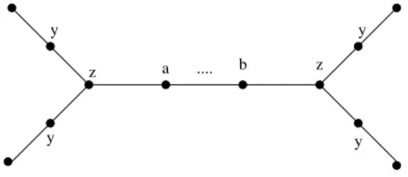
Lemma 5.7. Let Tn be a tree obtained from a path on n−8 vertices by gluing one-one
P5 at the middle vertices to both ends of the path Pn−8 (see Fig. 10). Then for any tree
Tm on m vertices we have
hom(Tm, Tn)>(n−1)2m−1.
Proof. We will show by induction on m that
hom(Tm, Tn)>(n−1)2m−1. (5.3)
Let v be any leaf of Tm with unique neighbor u and let Tm−1 =Tm−v be a rooted tree with root u. x y x y z a .... b z y y x x
Figure 10: Special double starlike trees.
Let us use the hom-vectors of the Fig. 10, that is
h(Tm−1, u, Tn) = (x, x, y, y, z, a, . . . , b, z, y, y, x, x). Now suppose that
hom(Tm−1, Tn)>(n−1)2m−2.
It is easy to see by induction that z >2x if Tm−1 has at least two vertices. By tree-walk
algorithm, we have hom(Tm(v), Tn) = 4x+ 8y+ 6z+ 2(a+· · ·+b) >8x+ 8y+ 4z+ 2(a+· · ·+b) = 2 hom(Tm−1, G) >(n−1)2m−1, which shows (5.3).
T T T T T T T 1 1 2 2 3 3 4
T
T’
T4 Figure 11: LS-switch.Next we introduce a transformation which we will call LS-switch (Large-Small switch).
Definition 5.8(LS-switch). LetR(u, v) be a tree with specified verticesuandvsuch that the distance ofuandv is even andRhas an automorphism of order 2 which exchanges the verticesuandv. LetT1(x), T2(x), T3(y), T4(y) be rooted trees such thatT2(x) is the rooted subtree ofT1(x) andT4(y) is the rooted subtree ofT3(y). Let the treeT be obtained from the treesR(u, v), T1(x), T2(x), T3(y), T4(y) by attaching a copy ofT1(x), T4(y) toR(u, v) at vertex uand a copy ofT2(x), T3(y) at vertex v. Assume that the treeT′ is obtained from
the trees R(u, v), T1(x), T2(x), T3(y), T4(y) by attaching a copy of T1(x), T3(y) to R(u, v) at vertexuand a copy ofT2(x), T4(y) at vertex v. ThenT′ is the LS-switch ofT. Observe
that there is a natural bijection between the color classes of T′ and T.
A particular case of the LS-switch is when R(u, v) is a path of even length with end vertices u and v, T2(x) and T4(y) are one-vertex rooted trees, then T′ is obtained from T by an even-KC-transformation, i.e., KC-transformation according to a path of even length. Another useful special case is when R(u, v) is a tree where we attach an arbitrary tree to the middle vertex of the path on 3 vertices and u and v are the end vertices of the path (in this case the automorphism simply switches u and v), and T2(x), T4(y) are the rooted trees with 1 vertex, in this case we get back to a particular case of the original
Kelmans-transformation [12].
The following theorem with respect to the LS-switch is just an extension of the even case of Theorem 1.3.
Theorem 5.9. Let T′ be the LS-switch of T. Let H be an arbitrary tree. Then
hom(H, T)6hom(H, T′).
Proof. (Sketch.) The unique shortest path connecting allTi’s in T (orT′) will be denoted
by P2k, a path of even length with vertices labeled consecutively by 0,1, . . . ,2k. Without loss of generality, we can assume that 0 ∈ V(T1). For 1 6 j 6 2k−1, let Aj denote the component of T that contains the vertex j when we delete all edges of P2k. By the definition of LS-switch, the subtrees Aj and A2k−j are isomorphic, so we can identify
V(Aj)\ {j}with V(A2k−j)\ {2k−j}. We will also consider V(T2)\ {0,2k}as the subset of V(T1)\ {0,2k} and V(T4)\ {0,2k}as the subset of V(T3)\ {0,2k}.
Let v be a vertex of H. For 0 6 s 6 2k, u ∈ V(Ti)\ {0,2k} (1 6 i 6 4) and
a∈V(Aj)\ {j} (16j 62k−1), we define
ps :=|{{f ∈Hom(H, T) :f(v) = m}|, p′s :=|{{f ∈Hom(H, T′) :f(v) = m}|,
ti(u) :=|{f ∈Hom(H, T) :f(v) =u}|, ti′(u) :=|{f ∈Hom(H, T′) :f(v) =u}|,
and
pj(a) := |{f ∈Hom(H, T) :f(v) = a}|, pj′(a) :=|{f ∈Hom(H, T′) :f(v) = a}|.
We prove by induction that the following inequalities are preserved by the steps of the tree-walk algorithm. For any 06s6k,a∈V(Aj)\ {j}(16j 6k),u∈V(T2)\ {0,2k},
w∈V(T4)\ {0,2k}, x∈V(T1)\V(T2) and y∈V(T3)\V(T4) we have p′k−s+p′k+s>pk−s+pk+s and p′k−s >pk+s, pk−s (5.4) p′ j(a) +p′2k−j(a)>pj(a) +p2k−j(a) and p′j(a)>p2k−j(a), pj(a) (5.5) t′1(u) +t′2(u)>t1(u) +t2(u) and t′1(u)>t1(u), t2(u) (5.6) t′3(w) +t′4(w)>t3(w) +t4(w) and t′3(w)>t3(w), t4(w) (5.7) t′1(x)>t1(x) and t′3(y)>t3(y). (5.8) We only need to check that the two operations in the tree-walk algorithm preserve all the above inequalities, which is routine and left to the reader.
Now assume that Tn has two vertices, x and y, of degree 3. Among these trees (n vertices, 4 leaves, two vertices of degree 3) let us choose Tn to be the one for which hom(Tm, Tn) is minimal and among these trees the length of the path is maximal.
Let the four leaves ofTn denoted byz1, z2, z3, z4 such thatz1, z2 are closer toxthany, and z3, z4 are closer toy thanx. Let the number of edges of xP y, xP z1, xP z2, yP z3, yP z4
be a, b, c, d, e, respectively. We show that max(b, c, d, e)62. Indeed, if say b >2 then Tn can be obtained by an LS-switch from a graph T∗
n as follows.
Ifbis even, then letube the unique vertex such thatd(z1, u) = 2. ThenuP x=R(u, x) is a path of even length. Let T2 =z1P u. Furthermore, let T1 be the tree spanned by the
vertices x, z3, z4. T3 = xP z2 and T4 ={u}. Then T2 is a rooted subtree of T1 and T4 is a rooted subtree of T3. Now making an inverse LS-swith we obtain T∗
n. By Theorem 5.9, we know that
hom(Tm, Tn)>hom(Tm, Tn∗) and in T∗
n, the vertices of degree 3, y and u, has distance a+b−2> acontradicting the choice of Tn.
Ifbis odd, then letube the unique neighbor ofz1and we repeat the previous argument. The distance of uand x is even again.
Hence we can assume that max(b, c, d, e) 6 2. If not all of them are 2, then we can use Lemma 5.6 to get that
hom(Tm, Tn)>(n−2)2m−1+ 2.
If b=c=d=e= 2, then we use Lemma 5.7 to obtain that
hom(Tm, Tn)>(n−1)2m−1 >(n−2)2m−1+ 2.
This completes the proof of Proposition 5.5.
5.3
Trees with 3 leaves
Lemma 5.10. (a) Let n =a+b+c+ 1, and min(a, b, c)>2. Then for any tree Tm on
m vertices we have
hom(Tm, Ya,b,c)>(n−2)2m−1+ 2.
(b) Let n=a+b+ 2, and min(a, b)>3. Then for any tree Tm on m vertices we have
hom(Tm, Ya,b,1)>(n−2)2m−1+ 2. Proof. (a) 1 4 9 6 4 1 1 4 6 6 1 1/3 1/2 1/4 3/4 1/2
Figure 12: Ya,b,c where min(a, b, c)>2 with a special Markov chain.
We can think to Ya,b,c with min(a, b, c) > 2 as follows: we consider Y2,2,2 and we
subdivide the edges between the vertex of degree 3 and its neighbors a few times. Let us write the weights 1,4,1,4,1,4,9 to the vertices of Y2,2,2 according to the figure and then
let us write weights 6 on the new vertices obtained by subdivision. It is easy to check that there is a unique Markov chain on Ya,b,c, where the stationary distribution is proportional to the weights. (In fact, we write a few transition probabilities on the figure.)
It is easy to check that H(P|Q) = log 2 and if N = 24 + 6(n−7) = 6(n−3), then
= 9 N log N 9 + 12 N log N 4 + 3 N log N 1 + 6(n−7) N log N 6 + + 2· 12 N log 2− 1 4log 4 + 3 4log 4 3 = logN 6 + 9 N log 6 9+ 12 N log 6 4+ 3 N log 6 1+ 24 N log 2− 1 4log 4 + 3 4log 4 3 = log(n−3) + 24 N log 3 2. Since log(n−2 +ε)−log(n−3) = Z n−2+ε n−3 dx x 6 1 +ε n−3 = 6 N(1 +ε)
we can choose ε= 4 log32 −1> 12 to deduce that
hom(Tm, Ya,b,c)>(n−2 +ε)2m−1.
This is already greater than (n−2)2m−1+ 2 form >3. The statement is trivial form 62.
(b) 4 9 12 16 12 12 9 4 12 4 1 1 1 3/4 2/3 1/2 3/8 1/2 1/2 1/2 1/3 1/4
Figure 13: Ya,b,1 where min(a, b)>3 with a special Markov chain.
We use completely the same argument as in part (a). We think toYa,b,1as a subdivision
of Y3,3,1 and use the Markov chain on the figure. Again we have H(P|Q) = log 2 and the
sum of the weights is N = 48 + 12(n−8) = 12(n−4). Hence
H(Q) + 2(H(D|Q)−H(P|Q)) = logN 12 + 12 N 11 3 log 3− 1 3log 2 . Since log(n−2 +ε)−log(n−4) = Z n−2+ε n−4 dx x 6 2 +ε n−4 = 12 N(2 +ε)
we can choose ε= 113 log 3− 13log 2−2>1.79 to deduce that hom(Tm, Ya,b,c)>(n−2 +ε)2m−1.
This is already greater than (n −2)2m−1 + 2 for m > 2. The statement is trivial for m= 1.
Remark 5.11. Since every Markov chains is reversible on a tree, there is a natural way to define a new Markov chain on a subdivided edge. Assume that the probabilities of the stationary distribution were qi, qj and pij, pji were the transition probabilities at the vertices i, j. Then qipij = qjpji (reversibility) and we can put a vertex r with weight 2qipij and pri = prj = 1/2 on the edge (i, j). Then the new stationary distribution will be proportional to the weights {qi |i∈V(T)} ∪ {2qipij}.
Theorem 1.6. Let Tn be a tree on n vertices. Assume that for a tree Tm we have hom(Tm, Tn)<hom(Tm, Pn).
Then Tn =Y1,1,n−3 and n is even.
Proof. Note that if Tn has at least 4 leaves then Theorem 5.5 implies that
hom(Tm, Tn)>(n−2)2m−1+ 2 = hom(Sm, Pn)>hom(Tm, Pn)
contradicting to the condition of the theorem. Hence Tn = Ya,b,c for some a, b, c. Ob-serve that if one of a, b, c is even then Ya,b,c can be obtained from Pn by an even-KC-transformation and then Theorem 1.3 implies
hom(Tm, Tn)>hom(Tm, Pn)
contradicting to the condition of the theorem. Note that if n is odd, then one of a, b, c is necessarily even and so we are done. From Lemma5.10we also know that min(a, b, c) = 1, say c = 1 and min(a, b) 6 2. But then min(a, b) = 1, because it must be odd. Hence
Tn =Y1,1,n−3 and n is even.
Remark 5.12. There is a treeTm for which hom(Tm, S4)<hom(Tm, P4). On Fig.14one
9 9 9 9 10 10 4 4 Figure 14: An example.
can see a rooted tree and its homomorphism vectors to S4 and P4. Now if we attach k
copies of this rooted tree at the root then for the obtained tree Tm we have hom(Tm, P4) = 2·4k+ 2·10k >4·9k = hom(Tm, S4) for large enough k.
6
Open problems
We collected a few open problems and conjectures in this section.
We first recall a conjecture from the Introduction, namely that there is no exceptional case in Theorem 1.6 if n >5.
Conjecture 1.7 Let Tn be a tree on n vertices, where n > 5. Then for any tree Tm we have
hom(Tm, Pn)6hom(Tm, Tn).
Note that to prove Conjecture 1.7, one only needs to prove that for any tree Tm we have
hom(Tm, Pn)6hom(Tm, Y1,1,n−3)
for n>6, where n is even.
There is also an open problem in Figure 4, if true, would provide an alternative proof of the first part of Theorem 1.8 (through Theorem 1.2).
Problem 6.1. Is it true that
hom(Pn, Tn)6hom(Tn, Tn) for every tree Tn onn vertices?
We believe that the answer is affirmative for this question. This question naturally leads to the following problem.
Problem 6.2. Characterize all graphsG for which hom(Pm, G)6hom(Tm, G) for all m and all trees Tm on m vertices.
Note that if G isd-regular, then hom(Pm, G) = hom(Tm, G) =|V(G)|dm−1. We have also seen that the inequality of Problem 6.2 is satisfied if G = Pn or Sn. Probably, it is hard to characterize these graphs. Maybe, it is easier to describe those graphs G for which the inequality of Problem 6.2 is satisfied for large enoughm.
The dual of Problem 6.2 is also natural:
Problem 6.3. Characterize all treesTm onm vertices for which hom(Pm, G)6hom(Tm, G)
for all graph G.
Probably, this is an easier problem than Problem6.2. Note that already Sidorenko [19] achieved nice results on this problem. Still the problem is far from being solved.
In light of the tree-walk algorithm, it would be interesting to develop an algorithm for computing the number of homomorphisms from bipartite graphs to any graph.
Acknowledgments
The first author is very grateful to L´aszl´o Lov´asz and Mikl´os Simonovits for suggesting to study the papers of Alexander Sidorenko. He also thanks Benjamin Rossman for the comments on the paper [21]. He is also very grateful to Bal´azs Gerencs´er for the useful discussion on Markov chains and entropies.
This research was partly done while the second author was visiting the Alfr´ed R´enyi Institute of Mathematics. He is very grateful to Mikl´os Ab´ert and the Institute for their hospitality and support. He also would like to thank Yanfeng Luo for introducing the graph homomorphisms and Jiang Zeng for all his encouragement during this work.
Special thanks goes to Masao Ishikawa for suggesting the name tree-walk algorithm.
References
[1] Sr. Arworn and P. Wojtylak, An algorithm for the number of path homomorphisms, Discrete Math., 309 (2009), 5569–5573.
[2] B. Bollob´as, Modern graph theory, Graduate Texts in Mathematics, 184. Springer-Verlag, New York, 1998.
[3] B. Bollob´as and M. Tyomkyn, Walks and paths in trees, J. Graph Theory,70(2012), 54–66.
[4] J.A. Bondy and U.S.R. Murty, Graph Theory, Springer-Verlag, New York, 2008. [5] T.M. Cover and J.A. Thomas, Elements of information theory, 2nd ed., John Wiley
& Sons, New Jersey, 2006.
[6] P. Csikv´ari, On a poset of trees, Combinatorica, 30 (2010), 125–137. [7] P. Csikv´ari, On a poset of trees II, J. Graph Theory, 74 (2013), 81–103.
[8] P. Csikv´ari and Z. Lin, Graph homomorphisms between trees, II: Path coloring trees, preprint, 2014.
[9] D. Dellamonica Jr., P. Hacell, T. Luczak, D. Mubayi, B. Nagle, Y. Person, V. R¨odl, and M. Schacht, Tree-minimal graphs are almost regular, J. Comb., 3 (2012), 49–62. [10] M.A. Fiol and E. Garriga, Number of walks and degree powers in a graph, Discrete
Math., 309 (2009), 2613–2614.
[11] C. Jagger, P. Stovicek and A. Thomason, Multiplicities of subgraphs, Combinatorica,
16 (1996), 123–141.
[12] A.K. Kelmans, On graphs with randomly deleted edges, Acta. Math. Acad. Sci. Hung., 37 (1981), 77–88.
[13] S. Kopparty and B. Rossman, The homomorphism domination exponent, European J. Combin., 32 (2011), 1097–1114.
[14] A.M. Leontovich, The number of mappings of graphs, the ordering of graphs and the Muirhead theorem, Problemy Peredachi Informatsii 25 (1989), no. 2, 91–104; translation in Problems Inform. Transmission 25 (1989) 154-165.
[15] J.L.X. Li and B. Szegedy, On the logarithmic calculus and Sidorenko’s conjecture, Combinatorica, to appear.
[16] Z. Lin and J. Zeng, On the number of congruence classes of paths, Discrete Math.,
312 (2012), 1300–1307.
[17] L. Lov´asz and J. Pelik´an, On the eigenvalues of trees, Per. Mathematica Hungarica,
3 (1973), 175–182.
[18] A. Sidorenko, A correlation inequality for bipartite graph, Graph Combin.,9 (1993), 201–204.
[19] A. Sidorenko, A partially ordered set of functionals corresponding to graphs, Discrete Math., 131 (1994), 263–277.
[20] R.P. Stanley, Enumerative combinatorics, Vol. 1, Cambridge University Press, Cam-bridge, 1997.
[21] B. Rossman and E. Vee, Counting homomorphisms from trees and cycles, 2006, unpublished manuscript.