On Optimizing Firewall Performance in Dynamic
Networks by Invoking a Novel
Swapping
Window
-based Paradigm
Ratish Mohana, Anis Yazidia, Boning Fenga, John Oommenb,∗
aDepartment of Information Technology, University College of Oslo and Akershus,
Oslo, Norway. bSchool of Computer Science,
Carleton University, Ottawa, Canada : K1S 5B6.
Abstract
Designing and implementing efficient firewall strategies in the age of the In-ternet of Things (IoT) is far from trivial. This is because, as time proceeds, an increasing number of devices will be connected, accessed and controlled on the Internet. Additionally, an ever-increasingly amount of sensitive informa-tion will be stored on various networks. A good and efficient firewall strategy will attempt to secure this information, and to also manage the large amount of inevitable network traffic that these devices create. The goal of this paper is to propose a framework for designing optimized firewalls for the IoT.
This paper deals with two fundamental challenges/problems encountered in such firewalls. The first problem is associated with the so-called “Rule Matching” (RM) time problem. In this regard, we propose a simple condition for performing the swapping of the firewall’s rules, and by satisfying this
con-∗Corresponding author
Email address:[email protected](John Oommen)
The fourth author is grateful for the partial support provided by NSERC, the Natural Sciences and Engineering Research Council of Canada. A preliminary version of this paper, with a brief sketch of the results, was presented atACM ICCNS ’16, the 2016 ACM International Conference on
Communication and Network Security, in Singapore, in November 2016.
Fourth author’s status: Chancellor’s Professor,Fellow of the IEEE, andFellow of the IAPR. This author can be contacted at: School of Computer Science, Carleton University, Ottawa, Canada : K1S 5B6. The author is also an Adjunct Professor with Agder University College in Grimstad, Norway. E-mail:[email protected].
dition, we can guarantee that apart from preserving the firewall’s consistency
and integrity, we can also ensure a greedy reduction in the matching time. It turns out that though our proposed novel solution is relatively simple, it can be perceived to be a generalization of the algorithm proposed by Fulp [1]. How-ever, as opposed to Fulp’s solution, our swapping condition considers rules that are not necessarily consecutive. It rather invokes a novel concept that we refer to as the “swapping window”.
The second contribution of our paper is a novel “batch”-based traffic es-timator that provides network statistics to the firewall placement optimizer. The traffic estimator is a subtle but modified batch-based embodiment of the Stochastic Learning Weak Estimator (SLWE) proposed by Oommen and Rueda [2].
The paper contains the formal properties of this estimator. Further, by per-forming a rigorous suite of experiments, we demonstrate that both algorithms are capable of optimizing the constraints imposed for obtaining an efficient firewall.
Keywords: Firewall Optimization, Matching time, Weak Estimators, Learning Automata, Non-Stationary Environments, Batch Update.
1. Introduction
The inter-connectivity, convenience and the all-prevalent digital services offered by the Internet, come with a steep price. As our society becomes more dependent on the Internet, the requirement to secure the information stored on these devices and services is more stringent and demanding. To secure the information, the users and systems’ administrators have to be even more security-conscious.
The filed of computer security is extensive. It encompasses the security of the physical machines as well as the information stored on them. However, in the context of the Internet, one has to be additionally concerned withnetwork -related aspects of security. Such a “specialized” form of security is mandatory
especially because an increasing number of devices are connected to various networks, and primarily to the Internet [3]. Network security deals with the se-curity aspects of data and communication within a/multiple network(s), and it spans many different concepts such as authentication, access policies, intrusion detection, intrusion prevention and honeypots/honeynets.
A first line of defence in network security is to use a firewall in order to enforce access policies. A firewall, in essence, is a system architecture program whose objective is to filter the incoming and outgoing packet traffic on a host or in a network. The task of accepting or denying access to the network is enforced by matching the header information of each data packet against a predefined set of rules, referred to as the “firewall policy”. Each rule has an action associated with it, for example, to either deny or accept access, and this action is what decides whether a packet is dropped or not.
A study of many Internet and private traces shows that the major portion of any network’s traffic matches only a small subset of firewall rules. This, in turn, implies that the frequency distribution for some of the traffic properties appears to be highly skewed [4]. Furthermore, when performing packet filter-ing, each rule in a firewall policy will usually be checked in a sequential order. Consequently, as the firewall policy increases in size, as any rule is often com-bined with a matching rule of a higher order, the overhead associated with the task of filtering the firewall, will become increasingly costly.
The reader will easily see that this rule matching phase can easily become a bottleneck in a high speed network when it is under attack or when it encoun-ters a heavy network load [1, 5]. Furthermore, it is well known that the com-puting power of hosts, the transmission speeds of packets and the complexity of networks, continue to increase. To keep abreast with these increasingly-demanding environments, firewalls must be able to “proportionately” adapt to changes by processing packets at increasingly higher speeds [6, 7]. Thus, it is desirable that a firewall monitoring system processes a lesser number of packet matches in order to reduce the potentially exorbitant filtering overhead as well as the overall packet matching time [4].
A natural inference of the above assertions is the following: In order reduce the number of packet matches that have to be processed, and to ensure that a firewall is able to process packets at an adequate speed, it is crucial for the firewall’s architecture to have an optimizedorderingfor the appropriate rules. This can be achieved by ensuring that the rule ordering is such that the rules that are matched most often, appear at the top (front) of the list of rules. This will reduce the amount of time used to process a packet by reducing the num-ber of required packet matches, and consequently reducing the packet filtering overhead. Additionally, it will also have the effect of improving the network’s throughput because a packet will spend less time being processed.
Although the problem is easily stated, the task of finding the optimal rule order is NP-hard because of inter-rule dependencies. Our goal is thus to find a heuristic algorithm to find a near-optimal rule order.
The complexity of the problem is accentuated by the fact that traffic patterns in networks are not static. This implies that since the patterns are dynamic and possibly time varying, one cannot learn the statistics of the traffic patterns using traditional estimation methods. Rather, one has to devise estimation (or learning) strategies that are rather effective for non-stationary environments. This is the task we undertake!
1.1. Problem Statement and Contributions
Put in a nutshell, this paper deals withdynamic networks, i.e., those that are characterized by being “under constant change and activity”. Essentially, a dynamic network is one in which the state of packet traffic is time-varying and non-stationary. This implies that the packet traffic fluctuates in such a way that no single type of traffic is dominant for an extended period of time. Our goal is to find a solution to the problem of optimizing theperformanceof a firewall in such dynamic networks. In order to achieve this, we attempt to answer the following questions:
• How can we optimize the order of the firewall rules in order to minimize the Rule Matching (RM) operations invoked?
• How can we learn and use the dynamic network traffic statistics to further opti-mize the firewall?
Of course, to achieve the above, we shall examine the traffic patterns statis-tically, combine the inferences with the workings of a RM algorithm. Thus, the major contributions of this paper are:
• We present an efficient and yet simple mechanism for optimizing the or-der of the rules in the firewall by using a novel concept that is referred to as theSwapping Window. TheSwapping Windowis a straightfor-ward strategy by which one can infer whether it is beneficial to swap theorderof two rules in a RM algorithm by considering their matching probabilities, and simultaneously guaranteeing that no inconsistencies are introduced in the firewall. We submit that, without loss of general-ity, our solution is a mapped efficient solution to theSingle Machine Job
Scheduling(SMJS) Problem [8] – since our problem can be shown to be a
specific instantiation of the latter.
• We present a novel adaptive algorithm for estimating the statistics of multinomial observations appearing in a batch mode4. The algorithm is able to deal with non-stationary environments and is an extension of the Stochastic Learning Weak Estimation (SLWE) work by Oommen and Rueda [2], which is, in and of itself, suitably adapted for high speed net-works. The observations that the estimation scheme receives are, in our case, the different matched rules within a time interval when they are examined as a “batched” data stream and not as sequential entities.
• We combine both the above-mentioned contributions (the rule ordering algorithm augmented with the estimation scheme) into a single algo-rithm so as to achieve a holistic approach for optimizing the firewall’s performance.
4The batched-mode version of Oommen-Rueda’s SLWE is a contribution in its own right to the field of estimation in non-stationary environments.
1.2. Organization of the Paper
After having introduced and motivated the problem in Section 1, we pro-ceed to review the related state-of-the-art in Section 2. In this section, we in-troduce the fundamental concepts and notations required for this paper to be a self-contained document. As well, in this section, as we will review the rele-vant related work. In Section 3, we present our solution composed of two main components: Rule Re-ordering (RR) and traffic estimation.
In Section 4, we present some theoretical results that demonstrate the va-lidity of the algorithms proposed in Section 3 for both rule ordering and esti-mation. Section 5 contains simulation results demonstrating the power of the scheme in stationary and dynamic environments. The experiments done for dynamic environments were based on a realistic test-bed, while those done for stationary environments were done using a simulated set-up (without requir-ing a test-bed). The paper also includes a thorough discussion of the results. Section 6 concludes the paper.
2. State-of-the-Art
This section outlines the current state-of-the-art when it concerns firewall optimization. It also introduces and explains several key concepts, technolo-gies and applications that we will use in this paper.
2.1. Firewalls
Based on the articleBenchmarking Terminology for Firewall Performance (RFC 2647)in [9], a firewall is defined as “a device or group of devices that enforces an access control policy between networks”. Firewalls are thus, devices or pro-grams that control the flow of network traffic between networks or hosts [10].
2.1.1. Rules and Packets
To understand how a firewall operates, it is necessary to understand the relationship between the access control rules and the packets that they govern. We now present a formal explanation of the relevant terms.
A firewall rule,r, is defined as ann-tuple of ordered fields:
r= (r[1], . . . ,r[n]), forn>1.
Although the upper bound ofnis network specific, for an Internet firewall, it is usually set to five and comprises of the following fields:Protocol,Source
Address,Source Port,Destination Address, andDestination Port[4, 11, 12].
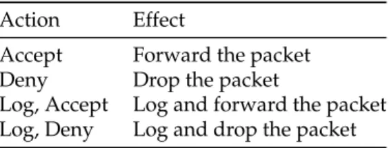
Each rule has an action field associated with it, and the value of the field de-cides the actions that the firewall will take when a match is found. Table 1 outlines the values of the action fields.
Action Effect
Accept Forward the packet
Deny Drop the packet
Log, Accept Log and forward the packet Log, Deny Log and drop the packet Table 1: The action field values of a firewall and its effects.
TheProtocolfield specifies a protocol as documented in the IP packet header’s
protocol field, as stated inInternet Protocol (RFC 791). For an Internet firewall, this would be either TCP, UDP or ICMP. However, it could also contain a wild card value (*), in which case it will match any protocol [10, 11, 13, 14]. The
AddressandPortfields specify the source and destination IP addresses, and
the source and destination port numbers of incoming and outgoing packets. Both of these fields can be configured to represent a range of values or a set of values, rather than only a single value. Tables 2 and 3 outline these types of configurations for the port and address fields respectively.
Notation Example Explanation
Wild Card * orany Port range 0 - 65535
Range 90-94 The given range of port numbers Single 90 A single given port number
Notation Example Explanation
CIDR 192.0.2.0/24 Address range 192.0.2.0 - 192.0.2.255 Wild Card 192.0.* Address range 192.0.0.0 - 192.0.255.255 Range 192.0.2.2 - 192.0.2.150 The given range of addresses
Single 192.0.2.2 A single given IP address
Table 3: Notation for the address field in a firewall rule.
A data packet,p, is defined as ann-tuple of ordered parameters:
p= (p[1], . . . ,p[n]),forn>1.
The upper bound ofnis limited by the fields defined in theInternet Protocol (RFC 791)[13]. That being said, not all fields in theIPheader are of importance for a firewall. Thus, a data packet, as seen by a firewall, is comprised mainly of the following fields [4, 11, 12]:
1. Protocol
2. Source Address IP 3. Source PORT
4. Destination Address IP 5. Destination PORT
These fields correspond to the fields that a firewall rule is comprised of and that it processes.
2.1.2. Firewall Policies
Afirewall security policydefines how an organization’s firewall handles
inbound and outbound network traffic based on its security policies. Prior to establishing these security policies, generally speaking [10], an organization should conduct a rigorous risk analysis in order to discover what types of traf-fic passes through its networks at all times. Based on such an analysis, the administrators should determine how they can secure it. Indeed, a firewall security policy is the result of implementing such an analysis .
Examples of policy requirements include accepting only necessary IP pro-tocols to pass [13], authorized source and destination IP addresses, authorized TCP and UDP ports to be used, and certain ICMP types and codes to be used [10]. Generally speaking, all inbound and outbound traffic that is not expressly permitted by the firewall policy should be blocked because such traffic is not needed by the organization. This practice can also have the additional bene-fit of reducing the risk of attacks and decreasing the volume of traffic carried into/through the organization’s networks [10].
To specify a formal definition for a firewall policy, let:
R={r1,r2,r3, . . . ,rN},forN>1
be the set of ordered firewall rules comprising a policy.
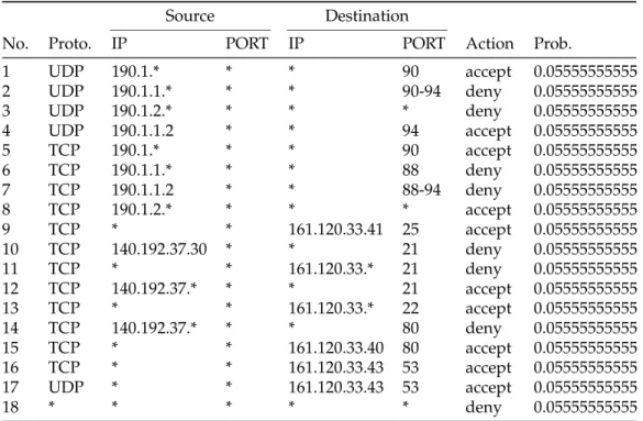
Such a firewall policy is considered to be comprehensive if any packet, p, has a match inR. In practice, this is achieved by implementing aDefault Rule
[4, 10] which serves the purpose of being acatch-allrule. It is usually added at the end of a policy and is designed such that it will simply discard any packet that has not matched any of the above rules. Table 4 shows an implementation of one such comprehensive firewall security policy.
2.1.3. Packet Matching
In many implementations of firewalls, the rules are stored internally as linked lists [12]. A firewall will, thus, generally speaking, sequentially compare a packet with a rule. In order for a rule,ri, to match a packet,p, the parameters
of the packet header must be a subset of all the permitted corresponding fields in the rule. Thus, if
ri[l], forl=1. . .n, and
p[l], forl=1. . .n
represent the ordered fields of the ruleri and the ordered parameters of the
Source Destination
No. Proto. IP PORT IP PORT Action Prob.
1 UDP 190.1.* * * 90 accept 0.05555555555 2 UDP 190.1.1.* * * 90-94 deny 0.05555555555 3 UDP 190.1.2.* * * * deny 0.05555555555 4 UDP 190.1.1.2 * * 94 accept 0.05555555555 5 TCP 190.1.* * * 90 accept 0.05555555555 6 TCP 190.1.1.* * * 88 deny 0.05555555555 7 TCP 190.1.1.2 * * 88-94 deny 0.05555555555 8 TCP 190.1.2.* * * * accept 0.05555555555 9 TCP * * 161.120.33.41 25 accept 0.05555555555 10 TCP 140.192.37.30 * * 21 deny 0.05555555555 11 TCP * * 161.120.33.* 21 deny 0.05555555555 12 TCP 140.192.37.* * * 21 accept 0.05555555555 13 TCP * * 161.120.33.* 22 accept 0.05555555555 14 TCP 140.192.37.* * * 80 deny 0.05555555555 15 TCP * * 161.120.33.40 80 accept 0.05555555555 16 TCP * * 161.120.33.43 53 accept 0.05555555555 17 UDP * * 161.120.33.43 53 accept 0.05555555555 18 * * * * * deny 0.05555555555
packetpcan be denoted as:
p⇒ri ⇐⇒ ∀l, p[l]⊂r[l], forl=1. . .n.
Informally speaking,pmatchesriifandonly ifall the parameters of pare in
a subset of the respective fields ofri. Because each parameterp[li]must match
the corresponding fieldri[lj], the order of fields in a rule is important to the rule
matching process. Thus, a packetpcan match multiple rules in a firewall,R. The matching policy of the firewall decides which rule render the packet to be considered to be “matching”.
There are, generally, three common matching policies used, namely, theBest Match,Last MatchandFirst Matchpolicies [15] listed below:
• Best Match: A packet is compared against allri∈R. The rule that matches
the closest with the packet is selected and its action is consequently exe-cuted.
• Last Match: A packet is sequentially compared to each rule ri∈R. The
last rule that matches,p⇒ri∈R, is selected and its action is consequently
executed.
• First Match: A packet is sequentially compared to each ruleri∈R. The
First rule that matches, p⇒ri∈R, is selected and its action is
conse-quently executed.
TheBest Matchand potentially, theLast Matchschemes increase the packet
matching time. Consequently, in this paper, we assume aFirst Matchmatching policy.
2.2. Firewall Modelling and Policy Anomalies
This section outlines how a firewall is modeled and what policy anomalies are.
2.2.1. Rule Intersection
As stated in Section 2.1.1, any parameter of a rule can contain a range of values. A consequence of this is that multiple rules can intersect. Two rules,ri
andrj, intersect if a comparison of their ordered parameters yields a nonempty
set. More formally, this is represented as below:
ri∩rj6=/0 ⇐⇒ ∃l, ri[l]∩rj[l]6=/0, forl=1. . .n.
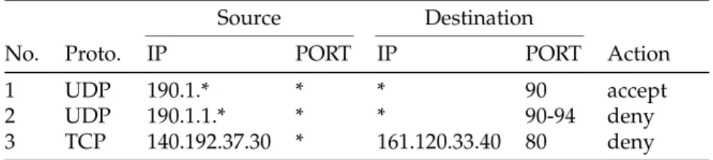
Consider Table 5 which displays some examples of this.
Source Destination
No. Proto. IP PORT IP PORT Action
1 UDP 190.1.* * * 90 accept
2 UDP 190.1.1.* * * 90-94 deny
3 TCP 140.192.37.30 * 161.120.33.40 80 deny
Table 5: Intersecting and non-intersecting rules.
Rules 1 and 2 intersect because Rule 2 describes a subnet in Rule 1. Fur-ther, the port in Rule 1 is a subset of the ports in Rule 2. In other words, the intersection of Rules 1 and 2 yields the following non-empty set:
{190.1.1.0−190.1.1.255,0−65535,0.0.0.0−255.255.255.255,90}.
On the other hand, Rule 3 is completely separate from the other two rules and does not intersect with them. The existence of rule intersections in a fire-wall policy can limit the size of the set of valid rule orderings and be the cause of anomalies in the policy.
2.2.2. Precedence Relationships
As described in Section 2.1.2, a firewall policy is defined as an ordered set of firewall rules,R, and each packet,p, will besequentiallycompared to a rule,
this is evident by the different types of matching policies that a firewall has. This means that theorderin which the rules are maintained and processed is important, and should be preserved. If the order is not preserved when the rules are re-ordered (for example, if they are, instead, reversed), a packet might match the wrong rule and violate the integrity of the policy.
The integrity of a policy is defined as the original intent of the policy. To formalize this, letRbe the original firewall security policy, and letR′be a re-ordering of all the rules inR. In that case, in order for the system to maintain the integrity of the firewall policyRinR′, a packet,p, must match the same rule and have the same action executed inR′as it would have done inR.
It is important for the reader to understand that a firewall is not merely comprised of disjoint rules. More often than not, there will bePrecedence
Re-lationshipsbetween many of the rules. A precedence relationship is a
connec-tion between two or more rules where a rule must appear before another in order for the integrity of the policy to be kept intact.
In order to accurately model a firewall policy with relationships, one uses a Directed Acyclic Graph,DAG G= (R,E), rather than a list. In such a model,R
represents the set of firewall rules in a policy andE, the set of directed edges, represents the set of precedence relationships between the rules. Representing a firewall policy using aDAGhas distinct advantages over a list representation. They are:
• The foremost advantage of a DAG representation is that it renders the task of modeling precedence relationships in a firewall much easier. This is because each node in the graph will represent a rule and each directed edge between two nodes will represent a precedence relationship. In-deed, an edge between rules is determined by finding the intersection between the rules in the firewall,R.
• Secondly, the problem of optimizing the rule order of a firewall has been shown to be comparable to that of thesingle machine job scheduling problem
be used to represent the scheduling problem, it would be appropriate to use a similar model in order to a model a firewall policy.
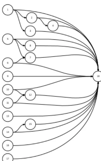
For clarification purposes, the precedence relationships specified in Table 4 are shown in Figure 1. As one can see, the figure displays theDAG, created (or rather, implied) by the relationships. In the interest of completeness, we now explain, in greater detail, two of the best-reported solutions for this problem.
Figure 1: A Direct Acyclic Graph (DAG) representation of a firewall security policy.
2.3. Firewall Matching Optimization: Legacy Approaches
In this section, we describe the relevant rule order optimization algorithms that are based on matching optimization, and outline the general problem of firewall Rule Re-ordering (RR).
The task of optimizing a firewall is comparable to that of solving the
Travel-ing Salesman Problem(TSP) [16] with precedence constraints [8]. The standard
TSP is defined as the task of finding the shortest route while traversing each city exactly once, given N cities and their intermediate distances. However, as observed by the author of [17], when constraints are included in the problem, it becomes more complex. The authors of [8] examined a variant of the TSP with
precedence constraints. This variant, known as the Time-Dependent Traveling Salesman Problem (TDTSP), considers the case when transition costs between two cities depends on the time of the visit5. This implies that certain cities can only be visited at a given time, and thus, trying to find an optimal path with such a constraint means that some cities must be visited before others due to the dependency relationships between the cites. This is precisely, a mapping of the problem of finding the optimal rule ordering in a firewall policy with dependency relationships, because finding the optimal rule ordering in a fire-wall entails creating a rule ordering such that some rules must be “visited” or compared against before other rules, until a match is found.
2.3.1. A Bubble Sort-like Algorithm
Since the problem is NP-hard, the author of [1], designed a simple heuristic algorithm, given in Algorithm 1, for optimizing firewalls rule ordering.
Algorithm 1:A simple Bubble Sort-like rule ordering algorithm.
Data:A list of firewall rules
Result:A new and improved ordering of firewall rules
1 done = False
2 while !donedo
3 done = True
4 for(i=1;i<n;i+ +)do
5 if(pi<pi+1ANDri∩ri+1=/0)then
6 interchange rules and probabilities
7 done = False
By studying the algorithm, one observes that it is similar to the Bubble Sort algorithm. It compares neighbours and, if possible, swaps them. Further [1], in order to preserve the rule precedence relationships, the algorithm uses rule probabilities and rule intersection as the swapping criteria. For example,
con-5The authors of [8] confirm that the TDTSP can be mapped ontosingle machine job scheduling
problem[8] which is known to be NP-hard [18]. Thus the optimization problem for firewall rules is also NP-hard. The only option to find the optimal solution requires an exhaustive search of the solution space — which is not a scalable solution. Rather, one must be content to find a sub-optimal solution using a heuristic algorithm.
sider the scenario when there are two rules, i.e., Rule1 and Rule2 where Rule1 has a lower probability than Rule 2, and where the rules don’t intersect. This means that the rules are not dependant on each other and are thus “swap-pable”. The algorithm will process the rules, in a pair-wise manner, until there are no more “swappable” rules.
The problem with this algorithm, however, is that one rule can prevent an-other from being ordered [1], rendering the algorithm to be unable to re-order groups of rules. The following is an example of this problem; suppose there are three rules, namely Rule1, Rule2, and Rule3. Rule 1 and Rule 3 have a dependency relationship, and the rules have the associated probabilities given in Table 6:
Rule Prob.
Rule1 0.1
Rule2 0.5
Rule3 0.4
Table 6: An example with a small number of rules with their probabilities.
Ideally, the rule with the highest matching probability would appear at the beginning of the list of rules in order to reduce the number of packet matches. Thus, in order to preserve the dependency relationships, the optimal rule order is: Rule1, Rule3, Rule2. However, the algorithm by [1] is not able to achieve this rule ordering, as explained below.
The algorithm will first swap Rule1 with Rule2. It will then check if Rule1 can be swapped with Rule3, but because they intersect, they will not be swaped. In the second iteration of the While loop the problem encountered becomes evident. Indeed, because Rule2 is better than Rule1 they will not be swapped, and further, because Rule1 and Rule3 intersect they will not be swapped either. Thus, when the algorithm terminates, the final order will be, clearly, subopti-mal6.
6This is a very simplistic example. Indeed, the possibility of terminating on suboptimal solu-tions is accentuated when the number of rules is larger.
However, despite its problems, this algorithm will still create a rule order-ing that is better than the original, if possible.
In the same vein (and inspired by the classical ascending-order sorting al-gorithms), Groutlet al. proposed a method [19] to optimize the performance of the firewall using rule re-ordering, and more particularly, swapping opera-tions. The method aspires to push the most accessed rules to the front of the firewall. However, the method suffers from a fundamental impediment when the rules are dependent. Unfortunately, the swapping algorithm proposed in [19] does not accommodate for the precedence relationships that might occur between the filtering rules which renders the problem to be NP-hard. In this paper, we, on the other hand, propose a simple condition that can be perceived as aSwapping Windowmechanism, and that ensures that no precedence con-straint is violated.
2.3.2. A DAG-based Algorithm
The authors of [14] presented a heuristic algorithm for optimized policy RR that is able to re-order a policy containing precedence relationships (or a sub-graph in theDAG) in such a way that the policy integrity is maintained. A short synopsis of the most important aspects of this algorithm is given below.
The algorithm functions by operating on certain data structures. It needs a set,G(ri), of rules containing the sub-graph rules ofri, i.e. the dependency
relationships forri. It also uses a FIFO Queue,S, to represent the optimal
pol-icy rule sorting, whereS is initially empty. Additionally, it requires a list,Q, containing the rules to be sorted, and this list is initially equal to the original firewall policy,R.
For each pass, the algorithm selects the rule with the highest average sub-graph probability from the sub-graph of rules available duringthat particularpass. The selected rule is then inserted into the list of sorted rules, S, if it has no rules dependent on it. Otherwise, the algorithm iteratively sorts the subgraph of its dependents until it finds a rule that has no dependent rules and inserts that rule into the list of sorted rules. The algorithm then updates the respective
data structures and repeats the process until all the rules have been placed in
S.
3. Proposed Solution
3.1. Overview of the Solution
The goal of this paper, as expressed in the problem statement, is not merely to create a rule ordering algorithm. Rather, our aim is to explore the problem of optimizing a firewall’sperformancein adynamic network. This means that for the firewall to have an optimised performance at all times, there needs to be an explicit understanding of when the rules have to be re-ordered as the network traffic dynamically begins to favour other rules in the policy.
This implies the need for two algorithms: The first algorithm must be useful to achieve the necessary RR, and the second one must be capable of updating the rule probabilities as the network traffic fluctuates. From an overall perspec-tive, we also need a single scheme that connects both these algorithms into a single, optimized adaptive firewall. We first consider the requirements for both these algorithms.
• The RR algorithmshould to be able to sort a firewall’s rule order based
on each rule’s matching probability, dependency relationships, and fire-wall position. This will ensure that the average packet matching time is reduced. In order to satisfy these criteria, the algorithm will need to have access to the current firewall security policy, a knowledge of the depen-dency relationships, and the matching probabilities of every rule. The details of this algorithm are presented in Section 3.2.
• The traffic aware algorithm should be able to update a rule’s
match-ing probability dynamically as the network’s traffic state changes. This means that this algorithm will need to have access to the currently-applied firewall security policy and the current number of packet matches for each rule. In order to enable dynamic estimation of the rule matching
probabilities, we present a novel weak estimator, which is a central com-ponent of our approach, in Section 4.1.
• Finally, the above two algorithms must be combined in such a way that they can communicate with each other. The traffic aware algorithm needs to be able to update the probability associated with a rule, and this up-date must be reflected in the rules used by the RR algorithm. If this is not achieved, the RR will never be able to find the optimal rule ordering of the firewall when the traffic state of the network changes. Thus, we will, briefly, describe two mechanisms for triggering the RR, namely, periodi-cally and “performance triggered”. These are described briefly in Section 4.2, and in more detail in the section that reports the experimental results that we have obtained, Section 5.
The primary reason why the problem is complex is because the RR and traffic-aware criteria themselves may be conflicting. Indeed, rulerimay have
to precederjwith regard to the network’s security policy requirements, and yet
the probability ofrjbeing applied may be greater than that ofribeing applied.
However, we will consider the RR issue first.
3.2. The Rule Re-Ordering Algorithm
The algorithm that we propose for RR, uses as its foundation the simple RR algorithm described earlier and presented in [1], namely Algorithm 1. Our new strategy is shown in Algorithm 2. However, before we formally present the algorithm, we shall explain its rationale.
3.2.1. Rationale for the Algorithm
Quite naturally, the algorithm itself takes as its input, a list of rules. It also has a list of rules that each given rule mustprecede, and which each rule must
succeed. If these lists collectively formed aDAGthat represented asingle string
of connected edges with a single source and a single sink, the problem of re-ordering the rules would have been trivial. The problem is necessarily complex
because the set of lists ofprecedingandsucceeding nodes could be potentially conflicting. Our solution represents a heuristic scheme by which these conflict-ing requirements are resolved in the best possible manner.
To be more specific, the algorithm itself takes as its input, a list of rules. It also maintains two data structures.
• The preceding listof a rule,ri, contains all the rules that are dependent
onri. Essentially, this means thatri must appearbeforethe rules in the
preceding list in order to maintain the integrity of the policy.
• The succeeding listof a rule,ri, contains all the rules thatriis dependent
on. Analogous to the above, this means thatrimust appearafterthe rules
in the succeeding list in order to maintain the policy’s integrity.
Our algorithm contains two main loops that it iterates through. For every iteration of the outer loop, the inner loop will traverse the whole list. The reason for this is that the algorithm will compare the current element in the outer loop,rx, with the current element in the inner loop,ry.
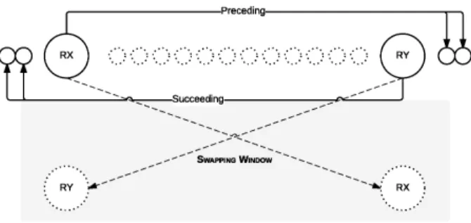
The algorithm will then try to find aswapping windowbetweenrxandry.
A swapping window is defined as an interval of positions in a firewall in which the two comparing rules can be swapped, without breaking the integrity of the firewall policy. The window is found by analyzing the two comparing rule’s succeeding and preceding lists.
By finding the rule with thehighestposition in the firewall in the preceding list forrx and the rule with thelowestposition in the firewall in the
succeed-ing list ofry, an interval of positions can be found. Once such an interval has
been determined, the algorithm will check if the window is a valid swapping window for the current rules being compared.
In order to check the validity of the swapping window, the algorithm will check if the current position ofrxis less than the lowest position in the
succeed-ing list ofryand if the position ofryis grater than the highest position in the
preceding list ofrx. If the latter expression is evaluated to beTrue, the swapping
However, the above is only valid ifrxhas a higher position in the firewall
thanry. In the case whereryhas a higher position in the firewall thanrx(as seen
in lines 12 and 13 in Algorithm 2) there is a slight difference in the swapping criteria. In this case, therx and ry values in the “If expression” switch places.
The swapping mechanism is illustrated in Figure 2.
Once the algorithm has found a valid swapping window and thus knows thatrx andrycan be swapped without violating the integrity of the policy, it
will do a simple comparison of the rules’ matching probabilities in order to de-cide whether they should be swapped or not. Even if the algorithm determines that they should be swapped, the algorithm will not properly swap them yet. Rather, the algorithm will do this based on a criterion value,∆new, explained
below.
The value∆newis created using the matching probability and position
num-ber of the rules being compared against and simply yields the estimated av-erage matching time before and after swappingrxandry. This can be said to
represent the swapping rank ofry. The higher the swapping rank, the more
optimal the swap is considered to be. Consequently, the algorithm will then perform a test to check whether this∆newvalue is greater than the current
max-imum value of∆, i.e.,∆max. If it is greater, then∆max is re-set to assume this
Figure 2: How Algorithm 2 re-orders rules.
When the inner loop has finished its traversal, a check is performed in order to find ifrxshould be swapped with a rule or not. If it should be swapped, the
rule with highest delta value,∆max, is chosen to be the optimal rule for it to be
swapped with. Finally, the outer loop will complete the iteration and move on to the next rule at which point the process above is repeated for that rule.
In essence, what this heuristic algorithm tries to achieve, is to get as many rules as possible, with a high matching probability, as close to the top of the firewall as possible.
The formal algorithm follows.
4. Theoretical Results: Estimation and Rule Ordering
4.1. Designing a Weak Estimator for Batch Updates
Having described our RR algorithm, we now proceed to the issue of traf-fic estimation, and design a Weak Estimator scheme that is relevant for batch updates. The algorithm that we propose is a modified version of theweak esti-matoralgorithm initially proposed by Oommenet al[20]. It is modified in such a way that it is able to use a batch of packet matches (as opposed to a single packet match as the SLWE scheme from [20] would do) in order to calculate
Algorithm 2:Our newly-proposed Rule Re-ordering algorithm.
Data:A list of firewall rules
Result:A new and improved ordering of firewall rules
1 forrx in rulesdo 2 ∆max=0
3 forry in rulesdo 4 ∆new=0
5 ifrx6=rythen
6 ifrx.pos<ry.posthen
7 ifrx.pos<succeeding max(ry)AND
ry.pos>preceding min(rx)then
8 ifrx.prob<ry.probthen
9 ∆new= (ry.prob−rx.prob)∗(ry.pos−rx.pos)
10 if∆max<∆newthen
11 ∆max=∆new
12 else
13 ifry.pos<succeeding max(rx)AND
rx.pos>preceding min(ry)then
14 ifry.prob<rx.probthen
15 ∆new= (rx.prob−ry.prob)∗(rx.pos−ry.pos)
16 if∆max<∆newthen
17 ∆max=∆new
18 if∆max>0then
19 swap(rx,ry)
the packet matching probabilities for a given rule. This ensures that the algo-rithm does not have to constantly perform estimate updates for each incoming packet.
The algorithm takes as its input a list of rules and a value for its parameter, λ. It then iterates through the list of rules and updates the probability associ-ated with each rule by using the modified weak estimator algorithm given be-low. Quite simply put, in order to update the probability associated with each rule, the algorithm calculates it using the previous probability of the given rule,
ˆ
pi, the total number of packet matches,M, and the number of packet matches
Algorithm 3:The Weak Estimator algorithm.
Data:A list of firewall rules, and a lambda value
Result:Updated probabilities for each rule in the list of rules
1 forruleiin rulesdo
2 pˆi=
mi
Mpˆi+λ(pˆi−
mi
M)
4.1.1. Theoretical Results: The Batch-oriented Weak Estimator
In this section, we present some theoretical results related to our algorithms. The first result concerned the optimality of the devised Batch-oriented Weak Estimator (Algorithm 3) described above. The algorithm is a generalisation of the Stochastic Learning Weak Estimator (SLWE) proposed by Oommen and Rueda [20]. The main difference is that the Stochastic Learning Weak Esti-mator operates in an incremental manner, i.e., updates the estimates of the probabilities upon receiving every single observation. As opposed to this, the Batch-oriented Weak Estimator proposed here is able to handle a batch ofM
observations.
Specifically, letX be a multinomially distributed random variable, which takes on the values from the set{‘1’, . . . ,‘r’}. We assume thatXis governed by the distributionS= [s1, . . . ,sr]T as follows:
X=‘i’ with the probabilitysi, where r
X
i=1
si=1.
We assume that between two discrete time instantsnandn+1, we obtain a batch ofM concrete realisations of X. Let {x(n,1),x(n,2),x(n,3), ...,x(n,M)}
denote the batch ofM observations obtained between the time instantsnand
n+1. The intention of the exercise is to estimateS, i.e.,sifori=1, . . . ,rbased on the batch of observations. We achieve this by maintaining a running estimate
P(n) = [p1(n), . . . ,pr(n)]T ofS, wherepi(n)is the estimate ofsiat time ‘n’, fori=
1, . . . ,r. We omit the reference to time ‘n’ inP(n)whenever there is no confusion. Letmi(n)be the number of elements in the batch{x(n,1),x(n,2),x(n,3), ...,x(n,M)}
for whichX=‘i’. Formally,mi(n) = M
X
k=1
I(x(n,k) =1)whereI(.)is the indicator function. Then, the values ofpi(n),1≤i≤r, are updated in the following way:
pi(n+1) ←
mi(n)
M pi(n) +λ(pi(n)−
mi(n)
M ). (1)
The reader should note that the above algorithm is a generalization of Oom-men and Rueda’s original SLWE algorithm [20]. In fact, whenM=1, the above updated equation coincides with the original algorithm devised in [20].
The properties of the estimator are catalogued and proven below.
Theorem 1. Let the parameterSof the multinomial distribution be estimated byP(n)
at time ‘n’ as per equation (1). Then, E[P(∞)] =S.
Proof. The expected value ofpi(n+1)given the estimated probabilities at time
‘n’,P, is: E[pi(n+1)|P] = [ k M+λ(pi(n)− k M)] M X k=0 Prob(mi(n) =k) (2) = [k M(1−λ) +λpi(n)] M X k=0 Prob(mi(n) =k) (3) = (1−λ)pi+ (1−λ) M X k=0 k M M k ski(1−si)M−k (4) = (1−λ)pi+ (1−λ) M X k=0 k M M! k!(M−k)!s k i(1−si)M−k (5) = (1−λ)pi+ (1−λ) M X k=1 (M−1)! (k−1)!(M−k)!s k i(1−si)M−k (6) = (1−λ)pi+ (1−λ)si M X k=1 M−1 k−1 ski−1(1−si)M−k (7) = (1−λ)pi+ (1−λ)si M X l=0 M l sli(1−si)M−l (8) = (1−λ)pi+ (1−λ)si. (9)
mulinomial distribution theorem in order to obtainProb(mi(n) =k). Further, in
Eq. (8), we have invoked a change of the variablek, wherek−1=l. Finally, in Eq. (9), we have applied the binomial theorem.
Taking expectations a second time, we have:
E[pi(n+1)] = (1−λ)si+ (1−λ)E[pi(n)]. (10)
Asn→∞, both equations E[pi(n+1)]and E[pi(n)]converge to E[pi(∞)], and
can be written:
E[pi(∞)](1−λ) = (1−λ)si (11)
⇒E[pi(∞)] = si. (12)
The result follows because (12) is valid for every componentpiofP.
The next result deals with the rate of convergence of the mean of the esti-mator.
Theorem 2. The rate of convergence ofPisfullydetermined byλ.
Proof. The proof follows directly from the corresponding proof in [20]. It is omitted to avoid repetition.
4.2. Theoretical Results: Triggering Rule Re-ordering
For triggering the decision to attempt RR in a dynamic environment, we will use two types of approaches: Schedule-based rule ordering and Performance-triggered rule ordering. In simple terms, the Schedule-based RR will re-order the rule after a fixed number of packets have been received. On the other hand, the Performance-triggered RR will re-order the rules whenever the per-formance of the current policy degrades. Obviously, the problem with Schedule-based approaches is that of determining the periodicity of change. While chang-ing the rule orderchang-ing too frequently results in unnecessary computation, if it is changed with too low a frequency, it results in a system that is unable to
track the environments. As opposed to this, Performance-triggered ordering can avoid both these trends if a degradation can be detected. However the efficiency of such a scheme is dependent on how fast the degradation can be detected, which is actually quite related to resolving the change detection prob-lem.
These two forms of mechanisms for triggering the RR, i.e., either periodi-cally or Performance-triggered, are described in detail in the experimental re-sults, Section 5.
With regard to Algorithm 2 we now prove a central result related to the condition that we use for swapping two rules, namely∆new. We will show that
∆newis simply the difference between the average matching time before and
after swapping. Indeed, we will prove two important properties of the RR algorithm which are the following:
• Whenever a swapping is performed, the average matching time of the firewall is decreased;
• The swapping condition based on the concept of the swapping window will preserve the integrity of the firewall.
In what follows, we shall use the notation that for any rule ri, located at
positionri.pos, the associated probability of it being invoked isry.prob.
4.2.1. The Swapping Condition
Theorem 3. The difference of the average matching time before and after swapping
two rulesrxandryis given by:∆new= (ry.prob−rx.prob).(ry.pos−rx.pos)
Letrk.posbe the position of rulekbefore swappingrxandry, and letrk.pos′
be the position of rulekafter swappingrxandry. It is easy to note that:
• rk.pos=rk.pos′ifk6=xandk6=y, and that
• rx.pos′=ry.pos
∆new = The Average time before Swapping−The Average time after Swapping = N X k=1 rk.prob·rk.pos− N X k=1 rk.prob′·rk.pos
= (rx.pos rx.prob+ry.pos·ry.prob)−(rx.pos′·rx.prob+ry.pos′·ry.prob)
= (rx.pos rx.prob+ry.pos·ry.prob)−(ry.pos·rx.prob+rx.pos·ry.prob)
= rx.pos(rx.prob−ry.prob) +ry.pos(ry.prob−rx.prob) = (ry.prob−rx.prob)·(ry.pos−rx.pos).
Note that ∆new= (ry.prob−rx.prob)·(ry.pos−rx.pos) = (rx.prob−ry.prob)·
(rx.pos−ry.pos).
The theorem is thus proven.
4.2.2. Preserving Policy Integrity: Consistent Rule Re-ordering
Theorem 4. A rulerk does not introduce inconsistency (i.e., it obeys all precedences
relationships) if:
preceding min(rk)<rk.pos<suceeding max(rk).
Proof. The reader will observe that obeying all the precedence relationships in which rulerkis involved in, reduces to two conditions:
• rk.posis less than any element in succeeding list ofrk
• rk.posis bigger than any element in preceding list ofrk.
The above two conditions can be written as: preceding min(rk)<rk.pos<
suceeding max(rk), proving the result.
Theorem 5.Ifry.pos<succeeding max(rx)ANDrx.pos>preceding min(ry), then
Proof. It is easy to prove that a rule rk does not introduce inconsistency if
preceding min(rk)<rk.pos<suceeding max(rk), implying that all the precedences
relationships are not violated.
Letrk.posbe the position of rulekbefore swappingrxandry, and letrk.pos′
be the position of rulekafter swappingrxandry. Further, observe:
• rk.pos=rk.pos′ifk6=xandk6=y, and that
• rx.pos′=ry.pos
• ry.pos′=rx.pos.
An inconsistency occursonlydue to either a violation due to the new posi-tion ofrxor due to the new position ofry. We will prove that the new position
ofrx, i.e.,rx.pos′, does not yield inconsistency. In other words:
preceding min(rx)<rx.pos′<suceeding max(rx).
By our hypothesis, we have ensured thatry.pos<succeeding max(rx)which
is the same asrx.pos′<succeeding max(rx). Since we have invoked the max
operator,rx.pos′, the new position is less than any element in succeeding list of
rx. Thus,rx.pos′<suceeding max(rk).
We shall now prove thatpreceding min(rx)<rx.pos′. We know that:
• rx.pos<ry.posis equivalent tory.pos′<rx.pos′ sincerx.pos′=ry.posand
ry.pos′=rx.pos;
• preceding min(rx)<rx.posimplies thatpreceding min(rx)<ry.pos′.
By combining the above two observations we obtain: preceding min(rx)<
ry.pos′<rx.pos′. We have thus proved thatpreceding min(rx)<rx.pos′.
Similarly, we can prove that the new position ofrywill not introduce
incon-sistency ifry.pos′ is less than any element in succeeding list ofrx. Hence the
result.
Theorem 6.Suppose that:rx.pos<succeeding max(ry)ANDry.pos>preceding min(rx)
5. Experimental Results
In this section we will describe the experimental results obtained by testing our algorithm on a rigorous suite of environments. The experiments were di-vided into two categories, those involvingStaticandDynamicenvironments respectively. While the static experiments were designed in such a manner that they were capable of only verifying the RR algorithm, the dynamic exper-iments verified the overall firewall optimizer. All together, we conducted six experiments, namely three static and three dynamic experiments.
5.1. Performance Metric: The Average Matching Time
The authors of [21] defined a metric describing the average matching time of an Access Control List (ACL). This metric can be applied to a firewall pre-cisely because a firewall policy is comprised of ACL rules with dependency relationships. The following describes how the metric is calculated.
Letθirepresent the matching probability of a ruleriinR. Then the average
matching time of the rule is:
ri∗θi
In other words to find the average matching time, we have to simply multiply the ruleri’s probability with its current position in the firewall. Extending the
above to the firewall, R, the average matching time of the firewall Rcan be denoted as,
N
X
i=1
ri∗θi, forN>1.
Thus, the average matching time is defined as the average number of rules that a packet must be compared against before a match is found. For example, if a policyRhas an average matching time of2.6, it means that on average,2.6
packets will be compared against the rules,{ri}, inRbefore a match is found.
From this, it is apparent that to optimize a firewall, the average matching time of the firewall must be low. By a simple analysis one sees that this can be
achieved by ensuring that the rules with high probabilities are at the top of the firewall.
5.2. Experimental Environment
The experiments were conducted on virtual machine instances created on theAlto Cloudcloud service at theOslo and Akershus University College of Applied Sciences. All the instances were obtained using anubuntu 14.14server image provided in the cloud.
In order to test the algorithms and the resulting firewalls, we needed two machines. Machine1 (M1) would run the firewall and the optimization algo-rithms. Machine2 (M2) would generate network traffic using a traffic gener-ating script. However, because the firewalls being tested contained rules with random source and destination IP addresses, the traffic generating script could not send the traffic through the internet because it would have been lost and never reached the firewall at M1. This was because there were no hosts in the environment that possessed those IP addresses. Consequently, in order to solve the problem, we needed a direct connection between M1 and M2. This connection was created by changing M2’s default gateway to the IP of M1 so that all traffic from M2 was routed through M1. This ensured that the spoofed IPs in the network traffic generated by the traffic generating script running on M2, would reach the firewall at M1. Figure 3 illustrates this.
5.3. Static Experiment 1: Intra-rule Re-ordering
The intention of this experiment was to provide proof that the algorithm for optimizing the RR was able to re-order the rules in such a way that the rules with the highest probability were at the top of the firewall while still maintaining the integrity of the policy. This experiment specifically tested RR within an intra-dependant group of firewall rules.
The experiment used a small policy of eight rules as described in Table 7. The rules{A - D} and{E - H} are intra-dependent but not inter-dependent.
Figure 3: Proposed firewall testing environment.
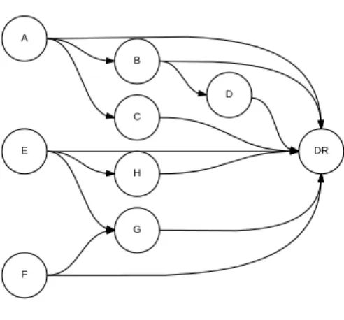
This means that there are only dependency relationships between the respec-tive rule groups{A - D}and{E - H}, but no relationships between the groups themselves. Figure 4 illustrates the relationships in Table 7 using aDAG.
Source Destination
No. Unique Name Proto. IP PORT IP PORT Action Prob.
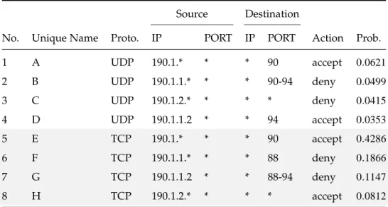
1 A UDP 190.1.* * * 90 accept 0.1147 2 B UDP 190.1.1.* * * 90-94 deny 0.0812 3 C UDP 190.1.2.* * * * deny 0.4286 4 D UDP 190.1.1.2 * * 94 accept 0.1866 5 E TCP 190.1.* * * 90 accept 0.0621 6 F TCP 190.1.1.* * * 88 deny 0.0499 7 G TCP 190.1.1.2 * * 88-94 deny 0.0415 8 H TCP 190.1.2.* * * * accept 0.0353
Table 7: The small firewall policy used for experiments in “Static Experiment 1”.
From Table 7 one observes that this is no optimal rule ordering. Rules C and D have a higher probability than the rules A and B, and thus, C and D should be placed higher up in the firewall as long as the integrity is maintained. Furthermore this configuration yields the firewall an average matching time of
Figure 4: The DAG of the small firewall policy used for experiments in “Static Experiment 1”. Here DR represents theDefault Rule.
5.3.1. Expected results: Static Experiment 1
The expected results from this experiment are the following: 1. Rule C should be placed higher up than rule B, but below rule A. 2. In spite of having a higher probability than rule B, Rule D should not be
placed higher up in the firewall because of the dependency relationship between rule B and D.
3. The average matching time will decrease when the policy is re-ordered for optimality. It should be2.6535.
5.3.2. Results Obtained: Static Experiment 1
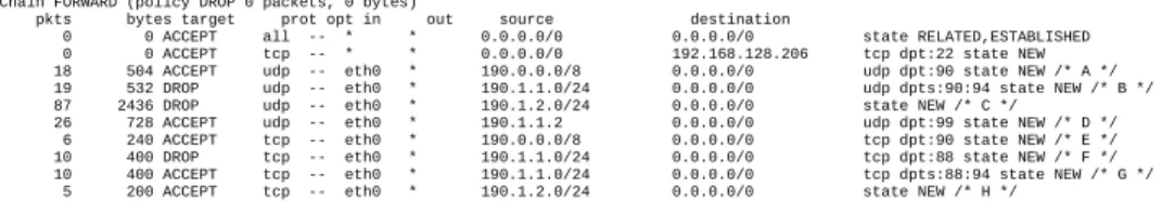
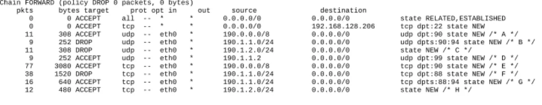
As mentioned earlier, the goal of this experiment was to show that the rule ordering algorithm was able to re-order rules while maintaining the integrity of the firewall policy. Figure 5 shows the initial conditions of the firewall.
Consider Figure 6. From this figure, it is apparent that rule C has been moved above rule B but below rule A. This is expected as there is no depen-dency relationship between rule B and C, but there is one between rules A and C which is why rule C must be placed below it in order that the integrity
! "" # # $ $ $ % $ $ $ % & ! '! (&)'* ! "" # # $ $ $ % +,-$+./$+-/$- . 0-- 1 +/ 2 3 ! "" # +, $ $ $ %/ $ $ $ % 0, 1 %# #% +, 24- "" # +, $+$+$ %-3 $ $ $ % 0, 0,3 1 %# ( #% /5 -34. "" # +, $+$-$ %-3 $ $ $ % 1 %# #% -. 5-/ ! "" # +, $+$+$- $ $ $ % 0,, 1 %# #% . -3 ! "" # +, $ $ $ %/ $ $ $ % 0, 1 %# #% + 3 "" # +, $+$+$ %-3 $ $ $ % 0// 1 %# #% + 3 ! "" # +, $+$+$ %-3 $ $ $ % 0//0,3 1 %# 6 #% 2 - ! "" # +, $+$-$ %-3 $ $ $ % 1 %# * #%
Figure 5: The FORWARD chain of iptables containing the firewall rules for Experiment 1.
of the policy is maintained. The average matching time reduced to2.6535, as expected. ! "" # # $ $ $ % $ $ $ % & ! '! (&)'* ! "" # # $ $ $ % +,-$+./$+-/$- . 0-- 1 ! "" # +, $ $ $ %/ $ $ $ % 0, 1 %# #% "" # +, $+$-$ %-2 $ $ $ % 1 %# #% "" # +, $+$+$ %-2 $ $ $ % 0, 0,2 1 %# ( #% ! "" # +, $+$+$- $ $ $ % 0,, 1 %# #% "" # +, $+$+$ %-2 $ $ $ % 0// 1 %# #% ! "" # +, $ $ $ %/ $ $ $ % 0, 1 %# #% ! "" # +, $+$+$ %-2 $ $ $ % 0//0,2 1 %# 3 #% ! "" # +, $+$-$ %-2 $ $ $ % 1 %# * #%
Figure 6: The FORWARD chain for Experiment 1 after Rule Re-ordering was achieved.
5.4. Static Experiment 2: Inter-rule Re-ordering
The intention of this experiment was to show how the rule ordering algo-rithm was able to re-order rules with no dependency while still maintaining the integrity of the policy. The experiment used a modified version of Table 7 where the intra-dependent rules,{E - H}had a higher probability than those of rules{A - D}. Table 8 illustrates the new table.
As can be observed from Table 8, the rules {E - H} should appear at the top of the policy, while rules{A - D} should be at the bottom. Because the groups of rules are independent from each other, the policy integrity should be maintained. The average matching time before optimization for this firewall
configuration is5.1427.
Source Destination
No. Unique Name Proto. IP PORT IP PORT Action Prob.
1 A UDP 190.1.* * * 90 accept 0.0621 2 B UDP 190.1.1.* * * 90-94 deny 0.0499 3 C UDP 190.1.2.* * * * deny 0.0415 4 D UDP 190.1.1.2 * * 94 accept 0.0353 5 E TCP 190.1.* * * 90 accept 0.4286 6 F TCP 190.1.1.* * * 88 deny 0.1866 7 G TCP 190.1.1.2 * * 88-94 deny 0.1147 8 H TCP 190.1.2.* * * * accept 0.0812
Table 8: The small firewall policy used for experiments in “Static Experiment 2”.
5.4.1. Expected results: Static Experiment 2
The expected results from this experiment are the following:
1. The rules{E - H}should appear at the top of the policy in the same order, while the rules{A - D}should be at the bottom, and in the same order. 2. The average matching time should decrease when the policy is re-ordered
for optimality. It should be2.6535.
5.4.2. Results Obtained: Static Experiment 2
The results obtained confirmed that the RR algorithm was capable of re-ordering non-dependent rules while maintaining the policy integrity of the firewall. Figure 5 shows the initial conditions of the firewall.
The results shown in Figure 8 were essentially as expected. Rules{E - H}
were at the top, as expected, while the rules{A - D}were at the bottom. The one difference from the expected results was that rule C was above rule B rather than the expected order of A, B, C and D. However, this is still a very positive result because our intent was to observe the re-ordering ofnon-dependentrules,
! "" # # $ $ $ % $ $ $ % & ! '! (&)'* ! "" # # $ $ $ % +,-$+./$+-/$- . 0-- 1 ++ 2 / ! "" # +, $ $ $ %/ $ $ $ % 0, 1 %# #% , -3- "" # +, $+$+$ %-4 $ $ $ % 0, 0,4 1 %# ( #% ++ 2 / "" # +, $+$-$ %-4 $ $ $ % 1 %# #% , -3- ! "" # +, $+$+$- $ $ $ % 0,, 1 %# #% 55 2 / ! "" # +, $ $ $ %/ $ $ $ % 0, 1 %# #% 2/ +3- "" # +, $+$+$ %-4 $ $ $ % 0// 1 %# #% +. .4 ! "" # +, $+$+$ %-4 $ $ $ % 0//0,4 1 %# 6 #% +- 4/ ! "" # +, $+$-$ %-4 $ $ $ % 1 %# * #%
Figure 7: The FORWARD chain of iptables containing the firewall rules for Experiment 2.
and thus, the intra-RR should have had no bearing on the outcome of the ex-periment. The average matching time was2.6619, which is slightly worse than the expected value of2.6535. The reason for this is that there were more packet matches for rule C than there were for rule B, in spite of the fact that rule B was characterized by a superior probability.
! "" # # $ $ $ % $ $ $ % & ! '! (&)'* ! "" # # $ $ $ % +,-$+./$+-/$- . 0-- 1 ! "" # +, $ $ $ %/ $ $ $ % 0, 1 %# #% "" # +, $+$+$ %-2 $ $ $ % 0// 1 %# #% ! "" # +, $+$+$ %-2 $ $ $ % 0//0,2 1 %# 3 #% ! "" # +, $+$-$ %-2 $ $ $ % 1 %# * #% ! "" # +, $ $ $ %/ $ $ $ % 0, 1 %# #% "" # +, $+$-$ %-2 $ $ $ % 1 %# #% "" # +, $+$+$ %-2 $ $ $ % 0, 0,2 1 %# ( #% ! "" # +, $+$+$- $ $ $ % 0,, 1 %# #%
Figure 8: The FORWARD chain for Experiment 2 after Rule Re-ordering was achieved.
5.5. Static Experiment 3: Comparing against Fulp’s Bubble Sort-like Algorithm
The next experiment was done to obtain a comparison between our RR al-gorithm and Fulp’s Bubble Sort-like rule ordering alal-gorithm [1] given in Sec-tion 2.3.1 and to understand the differences in the criteria when it concerns the resulting policy re-orderings. Here, the actual firewall IPtables scripts was not so crucial, since we were only interested in testing the rule ordering algorithms. The only information that both the algorithms needed were the dependency
relationships between the rules and the matching probabilities of the various rules.
The experiment used a program to generate DAGs in order to generate generic dependency relationships and probabilities. The experiment usedDAGs consisting of a 100 nodes (rules). The optimality was measured by calculating the average matching time of the resulting optimized firewall policies after each algorithm had applied its rule ordering on the policy.
5.5.1. Expected results: Static Experiment 3
The algorithm presented in [1] (and given in Section 2.3.1) does not take into account dependency relationships between multiple non-neighbouring rules, or the position of each rule within the policy when deciding to perform a swap. We can thus infer that it should generate policies with significantly worse av-erage matching times than the algorithm designed by us.
5.5.2. Results Obtained: Static Experiment 3
With regard to the data generation strategy in the the program that created theDAGs, there was a variable that decided on the probability (given in terms of a percentage) that a pair of rules would have a dependency relationship between them. In this experiment, we set the value of this percentage to 1% and 5%. The results of the experiments for these two values are shown in Tables 9 and 10 respectively. Also, the metric that was used to compare the algorithm from [1] and our RR algorithm was the average matching time.
Table 9 shows the result of five tests done using a 1% chance of edges on a graph with 100 nodes (or rules). First of all, we notice that the algorithm from [1] is not able to noticeably improve the average matching time. As opposed to this, our algorithm is able to significantly improve the average matching time. By way of example, the algorithm from [1] reduced the average matching time from34.8254to31.7256(by8.9%). As opposed to this, our algorithm had an average matching time of only11.788– a significant improvement of 66.2%. Indeed, it was62.8%better than the algorithm from [1].
Percentage Initial Our Algorithm Fulp Number of Rules 1 % 26.42 12.42 24.157 100 1 % 41.18 12.16 38.81 100 1 % 31.657 12.12 24.45 100 1 % 37.31 10.87 36.2 100 1 % 37.56 11.37 35.011 100
Table 9: A comparison of our algorithm with the one presented in [1] with theDAGcharacterized by a 1% chance of an edge between two nodes.
Regarding Table 10, the results obtained essentially state the same conclu-sion. The algorithm from [1] reduced the average matching time to 41.477
(from 42.2902, i.e., by 1.9%). Our algorithm, on the other hand yielded an average of25.5324, which was an improvement of39.6%. Comparatively, our algorithm was38.4%better than the one reported in [1].
Percentage Initial Our Algorithm Fulp Number Rules
5 % 41.98 22.87 41.33 100
5 % 30.28 21.321 29.06 100
5 % 46.371 27.701 45.52 100
5 % 33.7 21.71 33.115 100
5 % 59.12 28.06 58.36 100
Table 10: A comparison of our algorithm with the one presented in [1] with theDAGcharacterized by a 5% chance of an edge between two nodes.
Overall, we can conclusively state that our algorithm was significantly bet-ter than the one from [1]. However, understandably, we also noticed that the complexity of finding the optimal ordering increased with the density of the DAG. This is evident by observing that the average matching time in-creased significantly when the probability of having a directed edge between two nodes was increased (i.e., the graph was denser).
5.6. Dynamic Experiment 1: Schedule-based Rule Re-ordering with Dynamic Traffic
The intention of this experiment was to test both the RR algorithm and the Batch-oriented Weak Estimator algorithm in a dynamic network using a