Driving maneuver detection using knowledge distillation networks

(1)

Western University Western University

Scholarship@Western

Electronic Thesis and Dissertation Repository 3-6-2020 12:00 PM

Driving maneuver detection using knowledge distillation networks

Kyle Windsor

The University of Western Ontario Supervisor

Bauer, Michael A.

The University of Western Ontario Graduate Program in Computer Science

A thesis submitted in partial fulfillment of the requirements for the degree in Master of Science © Kyle Windsor 2020

Follow this and additional works at: https://ir.lib.uwo.ca/etd

Part of the Artificial Intelligence and Robotics Commons

Recommended Citation Recommended Citation

Windsor, Kyle, "Driving maneuver detection using knowledge distillation networks" (2020). Electronic Thesis and Dissertation Repository. 6844.

https://ir.lib.uwo.ca/etd/6844

This Dissertation/Thesis is brought to you for free and open access by Scholarship@Western. It has been accepted for inclusion in Electronic Thesis and Dissertation Repository by an authorized administrator of

(2)

Abstract

In this thesis, we examine the current state of Advanced Driving Assistance Systems (ADAS) and their relation to maneuver prediction in the literature. We then attempt to solve the problem of variable inter-driver behavior by applying a novel distillation learning system using RoadLab data on tracked driver cephalo-ocular gaze behavior in tandem with high-resolution CANbus data. Current training-based methods in maneuver prediction are potentially subject to underfitting as drivers may exhibit different behavior when prepar-ing to maneuver, but it has been shown that drivers can be grouped into at least two distinct behavior models. We use this information to personalize a deep neural network ensemble by distilling knowledge from a larger ”teacher” network to a smaller ”student” network. We change the networks’ input data to a subset of that data during training. Various groupings of driving sequence data are tested for prediction accuracy within this system, particularly against a validation driving sequence belonging to a specific driver group.

Keywords: Neural networks, maneuver prediction, distillation networks

(3)

Summary for Lay Audience

Advanced Driving Assistance Systems (ADAS) are systems implemented in ve-hicles composed of computer and sensory equipment that augment the driver’s natural abilities. These systems may provide indicators such as signals or addi-tional data feeds. Neural networks are a collection of mathematical operations that are applied in sequence to an input. They are distinct from simple equa-tions in that they can modify their own equation coefficients to try to mimic a desired output. Neural networks modify their own equations using many examples. Once the equation predictions are close enough to a desired output, they can be used with real-world inputs in place of examples to make accurate predictions.

In this thesis, we evaluate the use of distillation neural networks as a tool in ADAS. Particularly, we are using distillation networks to predict driver maneuvers. A driver maneuver may be a left turn, a straight driving sequence, or a right turn. If we represent these maneuvers as numbers, they can be used as example desired outputs for a neural network. As example inputs, we use the driver’s eye movement and some sensors (i.e. CANbus sensors, a standard sensor protocol) augmenting the vehicle.

A distillation network is a combination of multiple neural networks, where one network acts as a teacher, and the other acts as a student. When making predictions, the student factors the teacher’s predictions into its decisions. We

(4)

show that a well-trained student network works better for maneuver prediction than just a teacher network alone.

(5)

Acknowlegements

To my supervisor, Dr. Mike Bauer, and to my advisor, Dr. Steven Beau-chemin. Thank you both for all your guidance in completing this work.

To my friends and family, for your support and continued understanding. To Madhavi, thank you for your encouragement, enthusiasm, and wit.

(6)

List of Figures

2.1 The RoadLab instrumented vehicle. . . 11

3.1 A one-hot vector encoding of a left turn. . . 22

3.2 The interface of the RoadLab maneuver labeller. . . 24

3.3 The layout of the teacher neural network. . . 32

3.4 The layout of the student neural network. . . 32

4.1 Graph of a sample network loss vs. epoch count. . . 43

(10)

List of Tables

3.1 List of drivers recorded as a part of the RoadLab project. . . . 17

3.2 Route taken by each driver. . . 18

3.3 Maneuvers and frames in each driver sample. . . 23

4.1 Confusion matrix for dense neural network. . . 37

4.2 Driver sets used in neural network ensemble. . . 40

4.3 F1 scores for each of the frame spread amounts tested. . . 42

4.4 Preliminary F1 scores for each driver group. . . 45

4.5 Preliminary F1 improvement of student vs. teacher for each driver group. . . 45

4.6 F1 scores for increasing teacher weight at time-to-maneuver 0. 47 4.7 F1 change versus teacher for increasing teacher weight at time-to-maneuver 0. . . 48

4.8 F1 scores for increasing teacher weight at time-to-maneuver 1. 49 4.9 F1 change versus teacher for increasing teacher weight at time-to-maneuver 1. . . 50

(11)

4.10 F1 scores for changing time-to-maneuver at teacher weight 10. 51 4.11 Student scores vs. teacher scores for changing time-to-maneuver

at teacher weight 10. . . 52 4.12 F1 scores for changing teacher weight, with two validation drivers

at zero time-to-maneuver. . . 53 4.13 Student scores vs. teacher scores for changing teacher weight

with two validation drivers at zero time-to-maneuver. . . 54

(12)

List of Appendices

Appendix A Labelled Data . . . 69 Appendix B Neural Network Structure . . . 73

(13)

Chapter 1 Introduction

1.1 Overview

There are over 1.2 million fatalities per year due to road traffic incidents [23], and these incidents are the leading cause of death for those between the ages of 15-29. This quantity has been constant since 2007 [23]. The development of intelligent vehicles and driver assistance systems helps work towards the shared goal of decreasing the danger seemingly inherent to driving or being around vehicles. Advanced Driver Assistant Systems, or ADAS, aim to reduce the contribution of driver error to this risk [2].

For example, it has been argued in [7] that driver safety is an instance of task-capability interface, wherein an agent is at risk if the tasks they are

(14)

2 Chapter 1. Introduction

assigned are not in homeostasis with the agent’s capabilities; it is argued that the difficulty of a driving task is reducible to the driver’s vehicle speed. ADAS could suggest or enforce appropriate speed minima or maxima that match a driver’s maneuvering and perception capability.

An autonomous or intelligent vehicle is a vehicle that is fully self-controlled, and can be considered a self-driving vehicle. An augmented vehicle, however, is a vehicle that continues to rely on driver input, but provides sensory feedback and response to the driver’s actions and the environment. Augmented vehicles can be considered synonymous with ADAS.

An intelligent ADAS understands and utilizes the state of the driver, the vehicle, and the environment to perform its augmentation of the driving pro-cedure. The driver’s state corresponds to a driver model, wherein the driver model encapsulates the components of the driver to be used as input to the intelligent ADAS.

The overall goal of research into intelligent ADAS is to promote safety and security during motor vehicle operation.

1.2 Problem

Vehicle operation is an inherently dangerous action to take part in. Driving a vehicle requires training and licensing such that the vehicle can be safely

(15)

oper-1.2. Problem 3

ated by the driver. However, road accidents are a commonplace occurrence. A subset of road accidents are due to human error, where the vehicle operator is responsible for the accident, in contrast to faulty vehicle engineering. Despite the requirement for licensing in most countries, human error may be either be due to external stresses on the driver [3], perceptual problems, or a failure to cognitively process a situation [27]. Regardless, the employ of ADAS aims to reduce human error by providing automated tools to prevent such cognitive lapses by explicitly bringing a situation to the driver’s attention or altering the state of the vehicle in some way.

Machine learning and artificial intelligence have found use in various topics under the purview of ADAS [33]. Particularly, predicting road details and fea-tures are well-suited to neural network tooling [32]. A current problem with machine learning-based ADAS systems (and machine learning algorithms in general) is the lack of ability to train on small inputs. While the sample size of ”all drivers” is quite large, training a system to understand and interpret the model of a driver is nonsensical if drivers don’t exhibit common character-istics. It has been shown in the literature that different drivers are, in some ways, able to be clustered into similar groups [34] [12] [13] [22]. Ideally, we can ”personalize” these neural networks to the drivers themselves to avoid overgen-eralizing, particularly if different driver clusters exhibit similar characteristics which contrast other driver clusters’ behaviors.

(16)

4 Chapter 1. Introduction

1.3 Contribution

In this thesis, we present a novel application of knowledge distillation transfer in the context of vehicular maneuver prediction, with the goal of training a smaller ”student” neural network via the aid of a larger ”teacher” network. Given that it is possible to reliably categorize drivers into classes, we com-pare the choice of driver classification on the accuracy of the neural networks’ predictions of driver maneuvers. Specifically, we perform tests on various con-figurations of the ”teacher” and ”student” networks in relation to both their differences from traditional neural networks, such as how much influence the teacher’s output has on the student’s training, and to the classification of drivers used as input during teacher-student training.

In doing so, we obtain prediction accuracies of over 90% at various pre-maneuver points in time, and compare the examined parameters to determine which have a significant impact on the accuracy of the network. This thesis should not serve as a reference to find ”the best” distillation network for use with maneuver prediction, but only to examine which parameters used in distillation networks are useful in this specific use-case.

We also present a novel labelling tool developed to label driver maneuvers in RoadLab-style data. The tool was developed to assist in quickly labelling millions of frames of driving data such that maneuvers contained within them could be parsed by other predictive tools. We present a labelled catalogue of

(17)

1.4. Thesis Organization 5

653 driving maneuvers found in the RoadLab dataset. For details, please see Section 3.2.1.

1.4 Thesis Organization

This thesis is organized as follows:

In Chapter 2, we examine preliminary work in the field of ADAS maneuver prediction and related topics. In Chapter 3, we discuss the proposed architec-ture and model used to predict driver maneuvers. In Chapter 4, we present the implementation of the neural network ensemble and experimental setup. Finally, in Chapter 5, conclusions are presented and future work is discussed.

(18)

Chapter 2 Related Work

2.1 Adaptive Driver Assistance Systems

Adaptive Driver Assistance Systems, or ADAS, are a set of tools offering ”a means to enhance [...] active and integrated safety” [2]. The functions of an ADAS can be categorized into different levels: information, warning, control, and support [18], as they apply to vehicles and vehicle interaction with a driver. Intelligent ADAS, or i-ADAS, are ADAS that consider the driver’s state when performing augmentation.

Various methods of maneuver prediction are present in the literature. Be-cause driving has well defined patterns and laws, there are a variety of tech-niques, both artificial-intelligence based and otherwise [17]. Some involve the

(19)

2.1. Adaptive Driver Assistance Systems 7

usage of purely geometrical models wherein the potential patterns allowed by road geometry are mapped, as well as environmental factors such as traffic light status [9] [16]. When driver intent is contextualized and available, more statistical learning methods open up to be used by an ADAS, the simplest of which is the perceptron. These can either be direct, via head and gaze track-ing, or indirect, through other in-vehicle sensors such as turn signals, steering wheel angle, etc [21]. However, predicting driver intent is limited to the model of the driver state, which in practice is not fully determinable. In addition, despite predicting a driver’s maneuver, there may be unforeseen environmental factors such as the movements of other vehicles that may change the driver’s intent post-prediction.

One common feature present in ADAS is the use of driver maneuvers. Driver maneuvers can be predicted by incorporating driver gaze and head pose information (cephalo-ocular behaviour) [33] and can themselves act as a predictor of other behavior, such as checking for obstacles in the way of a maneuver or driving along a specific route.

There has been previous work regarding maneuver prediction using artifi-cial intelligence. Particularly, an IO-Hidden Markov Model was able to predict with relative accuracy the maneuvers taken by drivers, utilizing driver gaze, driver head pose, and CANbus data [33]. Incorporating driver gaze and head pose information (cephalo-ocular behaviour) improved time-to-prediction as

(20)

8 Chapter 2. Related Work

well as prediction accuracy.

2.2 Maneuver Prediction

First, we must identify our driver behavior model. Various driver behavior models were surveyed in [25]. The authors categorized driving models into the following four categories:

1. A focus is placed on the vehicle. The vehicle design, components, and dynamics are the primary factors in this category.

2. A focus is placed on the driver. Driver behavior and perception are the primary factors in this category.

3. A focus is placed on the overall system. Accidents and handling are treated as a large, holistic system.

4. A focus is placed on the environment. Other vehicles/traffic and envi-ronmental factors are examined for their impact on the driver.

In this thesis, we primarily identify the driver model as the second case, where we attempt to predict the maneuvers based on the driver’s behavior.

In [29], at the time of its writing, it was found that predicted driver maneu-vers can not be considered sufficiently safe. In particular, the authors found

(21)

2.2. Maneuver Prediction 9

driver behavior models do not account well enough for the variability in vehicle maneuvers external to the driver model itself to be considered adequate. As with any predictive mechanism smaller than the system it is predicting, the process of prediction is lossy and can never yield predictive results equal to that of its prediction target. The authors found the primary obstacle to good predictive results was a lack of sufficient data.

It has been shown in [20] that a variety of artificial intelligence algorithms have promise in predicting driver maneuvers. Fuzzy logic inference systems, hidden Markov models, and support vector machines have been assessed to predict driver maneuvers well. Machine learning and artificial intelligence’s role in ADAS has been shown, for example, in [8], where the utilization of a hidden Markov model lead to improved predictions by learning human driver traits.

In this work, maneuvers were identified as left turns, right turns, and straight driving sequences. In the context of this thesis, straight driving con-sists of all frames in a sequence that are not a part of left or right turns. In the literature, several types of maneuvers beyond these three have been exam-ined, such as lane changing [15] [19] or turning at intersections [5]. However, due to the size of our dataset, we decided to only consider these three simple maneuver groups.

(22)

2.3 Driver Grouping

In the literature, drivers have been shown to be able to be grouped into discrete sets based on their style of driving [34] [12] [13] [22]. Generally, this is based on either aggressiveness in maneuvers, or on fuel consumption [6]. Particularly, in [34], it was shown that drivers can be well-categorized into two distinct groups, where each group of drivers exhibit similar driving styles.

In this work we refer to the two groups as Group A and Group B. Group A exhibits more limbic driving characteristics (higher speed, less brake pedal force, higher acceleration, etc.) and Group B exhibits more calm driving characteristics (lower speed, more brake pressure, etc.) A detailed breakdown of the drivers for each group can be seen in Table 4.2.

(23)

2.4. Roadlab 11

2.4 Roadlab

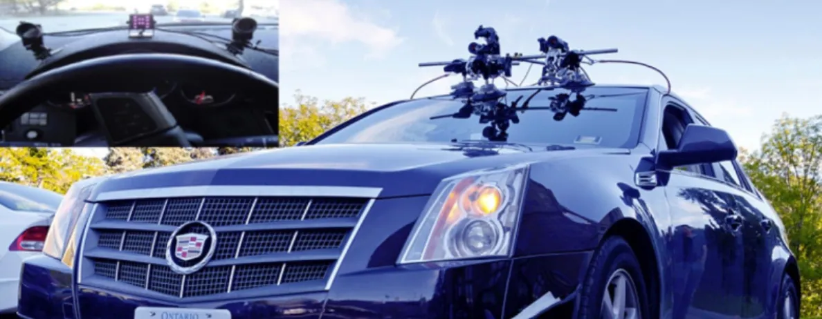
Figure 2.1: The RoadLab instrumented vehicle.

RoadLab is an augmented vehicle that provided data over 16 individual driving sequences, and is presented in [1] by Beauchemin et. al. RoadLab’s main ob-jective is to contribute to ADAS research by collecting various driver, vehicle, and environmental features in and around the augmented vehicle. The dataset RoadLab provides is used to minimize driver error through the detection and analysis of patterns stemming from driver behavior.

The RoadLab project collected data from an augmented vehicle (Fig. 2.1), containing an in-vehicle laboratory system. The laboratory was instrumented with an on-board diagnostic system (OBDII) via the CANbus protocol. Fea-tures collected include frontal stereoscopic video; driver head position and

(24)

angle; driver ocular parameters (i.e. direction of vision); vehicle dynamics such as brake pressure, speed, and steering wheel angle; and GPS positional data.

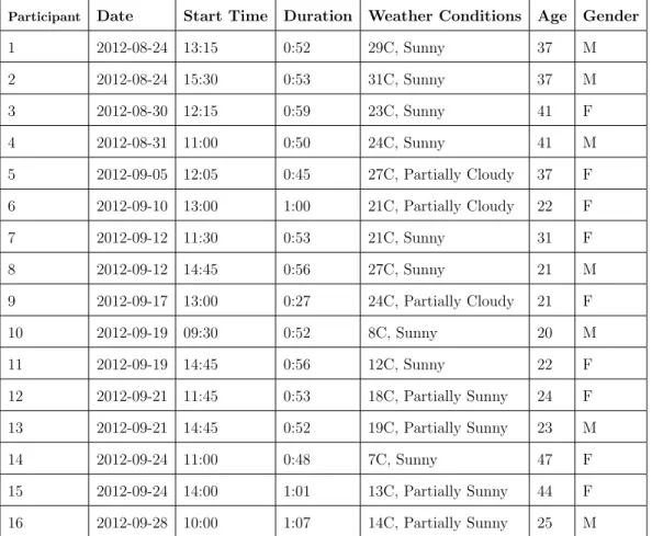
Data collection was performed over 16 drivers in London, Ontario, Canada, between the ages of 20 and 47. Drivers were assigned the same pre-determined route to navigate and the RoadLab laboratory collected ADAS data while they operated the vehicle. A second observer was present with the driver to monitor equipment and performance, as well as for navigation instruction. The drivers collected are listed in Table 3.1. In total, data collected involved 450 km of driving and weighs 3 TB. Instrumental CANbus data was collected at a rate of 60 Hz, while camera imagery was collected at 30 Hz.

2.5 Distillation Networks

Knowledge distillation networks are primarily used to compress neural net-works. Neural network ensembles can be composed of a very large number of parameters, so it is desireable to reduce the number of parameters in sit-uations where the input dataset is very large. In particular, neural network ensembles are compressed into a single neural network through the use of dis-tillation [11]. The first attempt at compressing a neural network was proposed by Bucila et. al. as a method to compress large neural network ensembles into

(25)

2.5. Distillation Networks 13

singular neural networks by training a neural network to mimic an ensemble’s output [4]. Since then, varying degrees of accuracy have been produced in neu-ral network compression. Distillation networks in particular were proposed by Hinton et. al. [11] as a means of compressing multiple highly-focused expert neural networks into a single well-rounded neural network.

Generally, neural network compression involves a small, ”student” neural network or neural network ensemble predicting the output of a much larger, ”teacher” neural network or ensemble. By utilizing a smaller neural network to predict the output of these large networks, fewer parameters are made available, and low-weight or highly general parameters are discarded. In the case of distillation, a smaller neural network predicts a larger neural network or ensemble while the larger neural network is still being trained. Thus, the smaller neural network can be trained not only on inputs and targets, but also on the teacher’s outputs and its similarity to the teacher.

Curiously, some distillation configurations also result in better network accuracy [26]. Improvements in network accuracy have been found by training thinner and deeper neural networks due to the high non-linearity occurring in such very deep neural networks. Knowledge distillation has been used before to transfer knowledge from a teacher to a student neural network [31], and has been found to not only outperform the teacher neural network, but also be trained faster. It was found that a student network trained via knowledge

(26)

distillation from a teacher network also generalizes to other related tasks better than if it was trained to perform the task with no precursory knowledge.

Deep residual networks are often utilized for the teacher and student layer architecture [10]. These knowledge distillation architectures, however, primar-ily apply to convolutional neural networks and as such may not hold for simpler non-convolutional networks, such as the one to be examined in this paper.

2.5.1 Lifelong Learning Networks

Varying the input over multiple epochs to distillation networks, or to neural networks in general, is not a common practice, except in the case of lifelong learning networks (for a survey, see [24]). The architecture of neural networks suggest they would perform best by training on a fixed, large set of data, with multiple epochs and shuffling, incorporating drop-out or similar overfitting mitigation techniques, etc. However, in the context of the problem we are examining, the inputs to the neural network may not be completely uniform: in other words, a neural network tries to be a ”jack of all trades”, despite the data potentially not being well-suited for this.

For example, consider a neural network that tries to predict a compass’ direction with inputs of the compass’ rotation relative to the ground, and the location of a nearby magnet, which can be either on the left or the right of the compass. While the network will likely learn from the compass’ rotation,

(27)

2.5. Distillation Networks 15

it will also take into account the nearby magnet, and thus the predictions will have two sources of error. However, if trained with the magnet consistently being on the left of the magnet, the network will ideally discard the magnet’s position, and so all error will be simply due to the compass’ rotation, thus reducing potential error.

Lifelong learning networks are networks that continually obtain potentially changing information over time. The challenge in designing and operating such a network is the problem of stability vs. plasticity, or choosing which information to discard and which to retain [14]. Neural networks typically tend to destructively forget more than they retain [28]. In this work, we will not be taking this into account, as the purview of that problem is well outside this thesis. However, the challenges posed by the forgetting problem are important to consider when evaluating the viability of varying inputs over multiple epochs.

(28)

Chapter 3 Data Processing and

Architecture

3.1 Data Collection and Organization

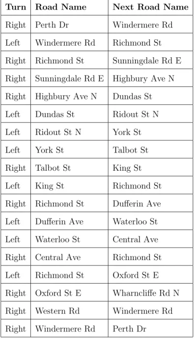
As described in Chapter 2, RoadLab is an i-ADAS system comprised of an augmented vehicle containing various sensors and trackers. The RoadLab project collected data for 16 individual drivers all navigating the same route. The drivers are presented in Table 3.1, and their route is presented in 3.1.

(29)

3.1. Data Collection and Organization 17

Participant Date Start Time Duration Weather Conditions Age Gender

1 2012-08-24 13:15 0:52 29C, Sunny 37 M 2 2012-08-24 15:30 0:53 31C, Sunny 37 M 3 2012-08-30 12:15 0:59 23C, Sunny 41 F 4 2012-08-31 11:00 0:50 24C, Sunny 41 M 5 2012-09-05 12:05 0:45 27C, Partially Cloudy 37 F 6 2012-09-10 13:00 1:00 21C, Partially Cloudy 22 F 7 2012-09-12 11:30 0:53 21C, Sunny 31 F 8 2012-09-12 14:45 0:56 27C, Sunny 21 M 9 2012-09-17 13:00 0:27 24C, Partially Cloudy 21 F 10 2012-09-19 09:30 0:52 8C, Sunny 20 M 11 2012-09-19 14:45 0:56 12C, Sunny 22 F 12 2012-09-21 11:45 0:53 18C, Partially Sunny 24 F 13 2012-09-21 14:45 0:52 19C, Partially Sunny 23 M 14 2012-09-24 11:00 0:48 7C, Sunny 47 F 15 2012-09-24 14:00 1:01 13C, Partially Sunny 44 F 16 2012-09-28 10:00 1:07 14C, Partially Sunny 25 M

(30)

18 Chapter 3. Data Processing and Architecture

Turn Road Name Next Road Name

Right Perth Dr Windermere Rd Left Windermere Rd Richmond St Right Richmond St Sunningdale Rd E Right Sunningdale Rd E Highbury Ave N Right Highbury Ave N Dundas St Left Dundas St Ridout St N Left Ridout St N York St Left York St Talbot St Right Talbot St King St Left King St Richmond St Right Richmond St Dufferin Ave Left Dufferin Ave Waterloo St Left Waterloo St Central Ave Right Central Ave Richmond St Left Richmond St Oxford St E Right Oxford St E Wharncliffe Rd N Right Western Rd Windermere Rd Right Windermere Rd Perth Dr

(31)

3.1. Data Collection and Organization 19

Video from the routes was collected at a rate of 30 Hz and a resolution of 320 by 240 pixels. Data from the CANbus systems was collected at 15 Hz. Each data frame contains the frame number and timestamp, latitude and longitude, GPS speed, vehicle speed, brake and gas pressure, engine RPM, steering wheel positioning, and left- and right-turn signal status. From these, additional derived data can be calculated, such as acceleration or statistical analyses (mean, standard deviation, etc.) It is expected that the neural net-work will perform these statistical functions, however, and as such they are not of consequence to this thesis.

In addition, head and gaze data was collected. Head tracking data consisted of a position and rotation both in Cartesian vectors. Gaze tracking was in the form of a 2-vector for each eye, containing pan and tilt angles. This was sampled at a rate of 30 Hz, as with video data.

Gaze tracking is very sensitive to error, so a variety of methods were em-ployed in the case of poor sensitivity. Optimally, driver irises were detected and used to extend an angle from the processed head angle. If this is unavail-able, the head angle is extrapolated and used as the gaze vector. Finally, if the head angle is unavailable, no gaze data is generated.

The fallback method used for gaze tracking was enumerated as the ’gaze quality’:

(32)

• 1 indicated that the gaze was cloned from the head rotation;

• 2 indicated that the gaze was calculated using visible image data; and

• 3 indicated that the gaze was calculated using IR image data. The gaze quality was included with each frame.

3.2 Maneuver Labels

RoadLab does not provide any maneuver information as-is. This is standard, as maneuvers are not a primary, quantitative feature that can be detected from an instrumented vehicle; they are a secondary feature to be extracted from primary features. As such, maneuver labels were to be manually placed over each maneuver. In particular, we needed to label specific frames as being a left-turn, right-turn or straight driving sequence (at random).

Straight movements cannot be realistically considered a maneuver under our three-maneuver classification model, as they consist of all frames that are not left- or right- turns. This would cause straight maneuvers to appear exag-geratedly long and the maneuvers would likely conflict with the end frames of a turning maneuver. If drivers’ behavior near the end of turning maneuvers is related to the turning maneuver itself, there may be some pressure on straight ’manevuers’ to be classified as those turning maneuvers. In addition, there

(33)

3.2. Maneuver Labels 21

are a significantly higher proportion of driving sequence frames that would be considered part of a straight maneuver compared to those that would be con-sidered part of a turning maneuver. To avoid these problems when our neural network ensembles were trained, we did not use each straight driving sequence as targets for our learning architecture. Instead, we randomly selected frames that were not a part of a left- or right-turn maneuver, and considered these frames straight maneuvers.

A left- or right-turn maneuver was considered to start when the vehicle began moving after stopping. The maneuver start position was only marked if the driver followed through their maneuver without stopping. In other words, if the driver was ”inching towards” a maneuver, we only marked a maneuver as ”started” when the driver initiated the actual turning sequence onto another road.

Each straight maneuver was one frame in length. This was chosen because the length of the maneuver is irrelevant to the prediction method we employ in this thesis: we only utilize the first frame of any maneuver (the ”start frame”) and use the frames leading up to it as inputs to our predictive network ensemble. To randomly select straight maneuvers, we picked a random frame from the driving sequence that was not a part of a left- or right-turn maneuver, or within 30 frames of the start or end of a left- or right-turn maneuver. In total, we collected 321 straight maneuvers.

(34)

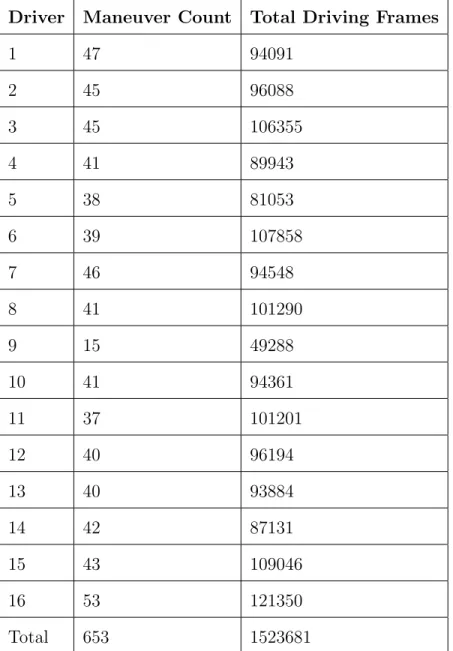
In total, 653 maneuvers were extracted over all 16 drivers. The maneuver counts per driver are presented in Table 3.3. Although maneuvers were col-lected with a start and end frame, we did not consider maneuvers in this thesis to have a duration as it is not in line with the selected goal. In this thesis, detecting a maneuver is equivalent to detecting the start of a maneuver. As such, the end frame and maneuver length were unused during experimentation.

A one-hot vector is a method of encoding classifications such that for a classC, its one-hot vectorVis defined asVi = 1 ifi=C andVi = 0 ifi6=C. V’s length is the number of classes to encode. An example one-hot vector is presented in Figure 3.1.

1 0 0

Figure 3.1: A one-hot vector encoding of a left turn.

The three maneuver classes were encoded as one-hot vectors of length 3 for use as neural network outputs in the distillation networks for each maneuver, and were coupled with the frame number where the maneuver started. As such there were 653 total one-hot vectors encoded.

(35)

Driver Maneuver Count Total Driving Frames

1 47 94091 2 45 96088 3 45 106355 4 41 89943 5 38 81053 6 39 107858 7 46 94548 8 41 101290 9 15 49288 10 41 94361 11 37 101201 12 40 96194 13 40 93884 14 42 87131 15 43 109046 16 53 121350 Total 653 1523681

(36)

3.2.1 Implementation

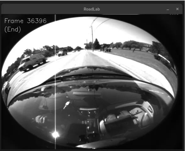
Figure 3.2: The interface of the RoadLab maneuver labeller.

A standalone C++ program was written to visualize and iterate over the frames of any RoadLab driver data sequence (a screenshot is presented in Fig. 3.2). It made use of the OpenCV 4 library to display a user interface. Frames

(37)

could be skipped individually using a keyboard, with ’fast’ keys skipping thirty frames. The frame number and maneuver, if it existed, were displayed in the user interface.

Possible maneuvers to identify were left turns, right turns and straight se-quences. Left and right turn maneuvers, consisting of a start frame and end frame, were inserted along each driver’s route. Some drivers performed addi-tional, non-route-based maneuvers, such as turning into a parking spot; these were treated identically to valid right- or left-turn maneuvers at intersections. When a maneuver was modified, all the maneuvers in the sequence were output to a comma-separated value file containing a maneuver enumeration, a start frame, and an end frame.

When starting the program, the user enters the driver number to read via a command-line option. The RoadLab binary file containing the specified driver’s recordings was read directly from disk and parsed to display a single frame. The user can use their keyboard to navigate between frames, as well as use their keyboard to label a frame as either a straight turn, right turn, left turn, or an end-of-previous-maneuver marker.

Upon start, if an existing output comma-separated-value file exists, the data in that output file is loaded to memory. Otherwise, an output file is created. When a maneuver or end-of-previous-maneuver marker is updated, both the output file and the in-memory data are updated with the new frame

(38)

and marker type. For an overview of the output format, please see Appendix A.

The data output from the implementation was used as prediction targets for the neural network ensembles used.

3.3 Data Processing

For the purposes of this thesis, video data was completely discarded, including both monoscopic and stereoscopic data. The reason for this was because in the context of distillation networks and the organization of the learning architec-tures to be used, image data is not a useful input into the system. While there are certainly useful aspects in manuever prediction predicted in image data [30], it is not covered in the scope of this thesis. In a way, image capture data is already reflected in the data, in that the gaze vectors obtained by the driver gaze tracker should indicate useful information in the environment, assuming the driver is looking with intent to make a maneuver. An example of a driver looking without intent might be a driver who is distracted by a pedestrian or other phenomena outside the driver model.

As video data was discarded, none of the cephalo-ocular data was rectified with respect to the camera’s intrinsic parameters, as it would be irrelevant when treated as a neural network input. The network should simply intuit the

(39)

3.3. Data Processing 27

non-linearity of rectification, if there was a need for this operation.

In order to facilitate the use of a neural network using the existing RoadLab data, some pre-processing was done. First, the camera output was divided into three vertical columns and two horizontal rows. Gaze data was sorted into six bins based on the X- and Y-angles from the average of both eyes’ rotations: top-left, top-center, top-right, bottom-left, bottom-center, and bottom-right. This was performed to provide a more stable input to the learning architecture we used. We hypothesized that maneuvers in a specific direction may be hinted at by a driver’s eye-vector: for example, many instances of a left-aiming eye rotation may indicate a left turn, and so using that data as neural network input would be useful.

Head rotational data was manipulated and grouped in the same way; head position was discarded, as it is unlikely to have a meaningful effect on the neural network. Of the CANbus feature set, we opted to include brake and gas pressure, engine RPM, left and right signals, vehicle speed, and steering wheel angle. These features were normalized to between 0 and 1 to prevent scaling problems with the network’s training functionality.

The gaze quality was also included as a training parameter, as the neural networks may learn to discard poor-quality gaze vectors.

Thus, in total, we had twelve dimensions as input to the neural network: a horizontal and a vertical bin for gaze vectors; a horizontal and a vertical bin

(40)

for head rotations; the gaze tracker’s quality; brake pressure; engine RPM; gas pedal force; left and right signal indicators; vehicle speed; and wheel rotation. This data was gathered and output to a comma-separated value file, and used in the network software written in Appendix B.

A frame window is a common input to neural networks based on video or other continuous data. It takes the form of an n×m matrix, where n is the number of dimensions of the input data and m is the length of the window in frames. Each frame’s input data vector is concatenated with the subsequent frames in order to utilize a video block as a neural network input.

A sliding window is a method to encode input to recurrent neural networks, wherein each discrete input to the network is a frame window, but the dataset consists of the entire sequence of data. Instead of inputs taking the form of discrete phenomena, a sliding window takes every frame in a sequence to be inputs to the neural network. Each subsequent input to the network is the previous input, with the next frame’s data in the sequence concatenated to the end of the frame window, and the oldest frame’s data removed. This is useful in cases where the network prediction is also continuous, such as financial data. Inputs to our neural networks were to take the form of frame windows. This seemed reasonable for the maneuver prediction problem. Despite the use of frame windows in this time-related prediction, one must be careful to not confuse the window matrix with a sliding window methodology. Because

(41)

3.3. Data Processing 29

maneuver input data is discrete and our problem is classification, the frame windows utilized are not sliding.

Each frame window consisted ofninput vectors as described in this section prior to a maneuver. Of interest is also how far ahead of time a maneuver can be predicted, so each frame window may or may not be immediately preceding the frame a maneuver occurs on; however, the both window size and amount of skipped frames was always consistent in one training session.

It is important to note that the input data was much smaller than a typical neural network training set (653 maneuvers). As such, some techniques were implemented to try and increase the training set. One method was to spread frame windows. If a maneuver occurred on framei, we also consider framesi±c

(c << i) to contain that same maneuver. Because c is small, the changes in parameters would also be small, but distinct. This borrows from the behavior of sliding windows, but is still distinct from them, as we are still only using very proximate frames to the actual event we are trying to predict.

If maneuver spreading is applied, the number of maneuvers is increased by however many frames we spread over. If we spread over cframes wherec≥1, the number of maneuvers in our dataset (and thus the number of inputs to our networks) becomes c×653.

(42)

3.4 Neural Network Architecture

We opted to use a distillation network ensemble. Distillation networks involve a large ”teacher” network and a smaller ”student” network. The teacher func-tions as any neural network, and the student does the same. However, the loss function is modified for the student network to penalize deviation from the teacher.

Defining a neural network’s predictions and actual targets as PN and TN respectively, the loss function of the teacher takes the form of

LT(P redicted, Actual) = Loss(PT,TT) (3.1)

Then the student’s loss function resembles

LS(P redicted, Actual) = Loss(PS,TS) +ω·Loss(PS,PT) (3.2)

where ω is a weight factor. The choice of actual loss function is up to the architect. As such, LS will be penalized not only by inaccuracy between its predictions and the true values input to the network, but also inaccuracy between its predictions and the teacher network’s predictions.

The teacher is trained for some epoch amount by itself. During this knowl-edge acquisition phase, no student activity is present. After this set duration, the student and teacher alternate training: the teacher will perform one epoch

(43)

3.4. Neural Network Architecture 31

of training, followed by the student, repeating for some fixed number of epochs. The differences between the teacher phase and the student-teacher phase are a subject of this thesis.

Any type of network can be used for this small ensemble, but we opted to proceed with a simple feed-forward neural network. Recurrent neural networks (including LSTM and GRU networks) were considered, but we chose near the beginning of the project to proceed with only feed-forward networks for simplicity. As such, inputs would consist of discrete, non-overlapping input window tensors and maneuver outputs. Utilizing time-series neural networks is a concrete area of future research, but would require changing the presented problem setup to one where maneuvers are not discrete or atomic.

In distillation networks, students are generally smaller than teachers in terms of overall neuron count. This is in line with the stated goal of distilla-tion networks, which is network compression. We chose to continue with this construction for simplicity. As the goal in maneuver prediction is accuracy, the student networks may be more performant with more neurons, but this is open for future work.

(44)

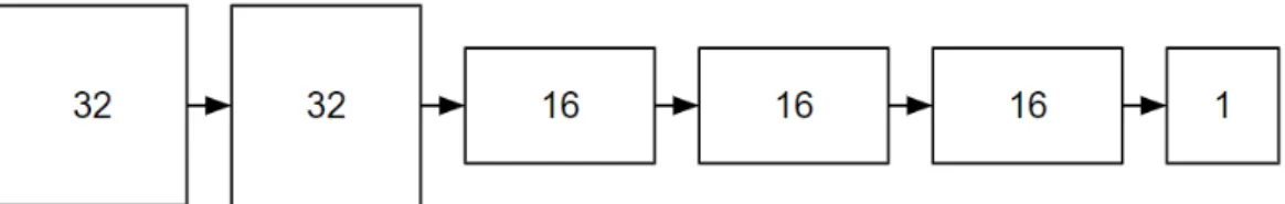
Figure 3.3: The layout of the teacher neural network.

Figure 3.4: The layout of the student neural network.

The feed-forward, dense teacher network and student network are por-trayed in Figures 3.3 and 3.4 respectively.

3.4.1 Performance Evaluation

To evaluate the performance of the networks involved, we used precision ac-curacy, recall accuracy and F1 scores for each.

A true positive prediction is a prediction which correctly predicted a result. A false positive prediction predicted a result to have occurred, which did not.

(45)

3.4. Neural Network Architecture 33

Likewise, a true negative is a prediction which correctly predicted the lack of a result, and a false negative incorrectly predicted the lack of a result.

The precision accuracy of a set of values where the true positive count is

tp and the false positive count is f p is defined in Equation 3.3:

Precision = tp

tp+f p (3.3)

It can be thought of as how trustworthy a network’s prediction of a maneu-ver is. That is, if a network predicts a target classification past a threshold, the precision score indicates how correct that prediction is. The recall accu-racy, where tp is the true positive count and f n is the false negative count is defined by Equation 3.4:

Recall = tp

tp+f n (3.4)

Recall can be considered the sensitivity of a prediction set (i.e. how fre-quently the network makes a prediction where a significant value actually exists). A network would have a high recall accuracy if it identifies most significant events.

Finally, the F1 score is the harmonic mean of precision and recall. It is defined in Equation 3.5:

(46)

F1 = 2· precision·recall

precision+recall (3.5)

The F1 score is used as a general purpose ”score” for the purposes of this paper and is taken to represent how accurate a specific neural network is.

(47)

Chapter 4 Maneuver Prediction

4.1 Neural Network Prediction

Before investigating if it is possible to create a neural network ensemble to pre-dict maneuvers, we must determine if neural networks can prepre-dict maneuvers at all. In previous work [33], it was shown IO-HMM models can predict ma-neuvers quite well; however, to test our deep neural network architecture, we will need to gauge maneuver predictability separately. For our neural network, we used a 40-frame window of driver metrics, consisting of:

• Gaze horizontal and vertical quadrant

• Gaze quality

(48)

36 Chapter 4. Maneuver Prediction

• Head direction horizontal and vertical quadrant

• Brake, engine, gas pedal, wheel angle metrics

• Left and right signals

• Vehicle speed

Maneuvers from Driver 1 were (arbitrarily) used as the validation set, and maneuvers from drivers 2 through 16 were used as inputs to the network. A different driver’s maneuvers could have been chosen as the validation set if desired. The neural network was composed of four dense layers with variable dropout layers in between to prevent overfitting. Training was performed over 12 epochs. Statistics (such as accuracy, F1 score, and confusion matrices) were calculated over 8 individual training runs for all neural networks presented in this paper; the mean of the 8 tests’ statistics are presented as the accepted values.

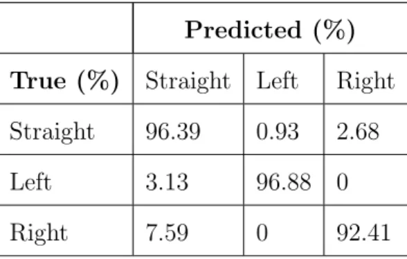
The confusion matrix for these neural networks are presented in Table 4.1. These values are not to be confused for F1 scores: they are percentages.

(49)

4.2. Experimental Setup 37

Predicted (%) True (%) Straight Left Right Straight 96.39 0.93 2.68 Left 3.13 96.88 0

Right 7.59 0 92.41

Table 4.1: Confusion matrix for dense neural network.

The average F1 score found via our dense network was 0.923. From the confusion matrix, we see left and right turn maneuvers were never confused, with all confusion occurring with straight maneuvers.

These results suggest driver maneuvers can be predicted reasonably well with a neural network.

4.2 Experimental Setup

Similar to the dense neural network in the previous section, various neural network configurations were designed to test multiple teacher-student ensemble networks. Equations 3.1 and 3.2 were used as loss functions to the two neural networks.

As the objective is to determine if neural networks can be personalized, we chose to offer different inputs at different times to the neural networks. In

(50)

general, teachers were to be trained for some Nt epochs on all drivers except the validation set of drivers. After this period elapses, students are introduced and trained forNsepochs. Key to the experiment were the inputs used during the student-training phase. To encourage the student to learn in a specialized manner, the input to the student differed from that of the teacher.

The reasoning behindNt epochs trained on specifically all drivers’ maneu-vers was to attempt to make the teacher network as broad and knowledgeable as possible. Group A doesn’t contain that many maneuvers, and as such we are attempting to imbue as much information as possible in the teacher network. The teacher network will then hypothetically distill the important information from this process to the student.

Our hypothesis was that if the student-training phase’s input was in the same class as the student, the student would exceed the teacher’s performance, as they would only learn information that is relevant to them.

During the student-training phase, teachers are also trained with the stu-dents to prevent excess penalty for stustu-dents deviating from the teacher.

Experiments varied over a variety of parameters and hyperparameters. Generally, teacher networks were deeper than student networks in terms of number of layers and layer width. The parameters and hyperparameters con-sidered included:

(51)

4.2. Experimental Setup 39

• Input maneuver frame spreading

• Time-to-maneuver

• Early stopping

• Teacher weight on student

• Teacher and student network layout

Most importantly, however, we decided to proceed primarily testing which driver sets to use for validation and prediction.

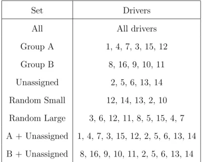
Driver sets are noted in Table 4.2. Group All consists of all drivers that were not a part of the validation set. Groups A and B are taken from [34], and Unassigned (or Group U) are the five excluded drivers taken from [34]. The unassigned group was excluded in that work due to diverging from the original route or being cut short; however, we assume they would have been assigned to A or B. Random Small and Random Large were randomly selected from the pool of Group All drivers, and A + Unassigned and B + Unassigned are the union of Group A or B and Unassigned.

(52)

Set Drivers

All All drivers

Group A 1, 4, 7, 3, 15, 12 Group B 8, 16, 9, 10, 11 Unassigned 2, 5, 6, 13, 14 Random Small 12, 14, 13, 2, 10 Random Large 3, 6, 12, 11, 8, 5, 15, 4, 7 A + Unassigned 1, 4, 7, 3, 15, 12, 2, 5, 6, 13, 14 B + Unassigned 8, 16, 9, 10, 11, 2, 5, 6, 13, 14

Table 4.2: Driver sets used in neural network ensemble.

Teachers were always trained on the All group during the teacher phase. Afterwards, a battery of tests over all groups and some parameters was per-formed, yielding statistics over an average of 8 trials. For all tests, we used an arbitrary frame window size of 40 frames, with precursory experimental tests indicating this length would contain the necessary data to predict a ma-neuver. Fewer frames than this yielded generally poor results, regardless of architecture. The 40 frames are not related to the length of the maneuvers, but rather the length of the frame window discussed in Section 3.3. We chose to not investigate longer frame windows to avoid overcomplicating our results, but there is room for future research in that area.

(53)

4.3. Results 41

If a time-to-maneuver value was non-zero, this indicates the frame window was shifted backwards in time, such that a time-to-maneuver of 2.0 seconds would indicate a prediction for frameF = 0 would use frames [−100,−60] (or, at 30 frames-per-second, a window consisting of frames between 3.33 and 2.0 seconds before the maneuver takes place).

4.3 Results

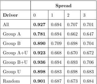
The first result found was that frame-spreading as discussed in Chapter 3 performed extremely poorly compared to not using frame-spreading (Table. 4.3). This can be attributed to driver behavior at the beginning of a maneuver vs. that of a driver during a maneuver vs. that of a driver prior to a maneuver. Drivers may exhibit very different behaviors in these three periods which may or may not align with that at the beginning of a maneuver. As such, for all future tests, frame spreading was not applied.

(54)

42 Chapter 4. Maneuver Prediction Spread Driver 0 1 2 3 All 0.927 0.694 0.707 0.701 Group A 0.781 0.694 0.662 0.647 Group B 0.890 0.709 0.698 0.704 Group A+U 0.923 0.668 0.670 0.672 Group B+U 0.936 0.694 0.693 0.706 Group U 0.898 0.683 0.698 0.683 Random 0.901 0.687 0.673 0.684

Table 4.3: F1 scores for each of the frame spread amounts tested.

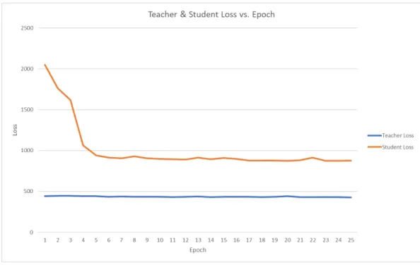
Initially, we planned to perform 30 or more epochs for each phase (teacher and student-teacher). Examining loss and accuracy metrics of the neural net-work at each epoch, we found that most neural netnet-works - both student and teacher - reached peak validation accuracy after 5 to 10 epochs (see Fig. 4.1). This is likely due to the problem’s simplicity and cleanliness of input data. We opted to use a teacher training length of 6 epochs and a teacher-student training length of 6 epochs.

During this evaluation we also found that the networks tended to not over-fit in either the large-epoch-count or small-epoch-count case. This can be attributed to the use of many dropout layers throughout the dense neural networks, preventing gradient problems.

(55)

4.3. Results 43

Figure 4.1: Graph of a sample network loss vs. epoch count.

It was found that there is generally no global correlation between Group A or Group A + Unassigned and a better prediction with a time-to-maneuver, versus other groups. In addition, Group A was not consistently more or less accurate than Group A + Unassigned.

At zero time-to-maneuver (Table 4.4), Group A was found to be compara-ble to the Random Large group in terms of the improvement on the F1 score of the teacher. Group A+U received the best F1 score at zero time-to-manevuer. Interestingly, Group A contained 215 maneuvers, whereas Random Large

(56)

con-44 Chapter 4. Maneuver Prediction

tained 370; this may indicate Group A performed stronger on a per-maneuver basis. Group A+U contained 419 maneuvers.

When normalizing over maneuver counts, groups U, Random Small, B, and A all performed the best. Each had a similar F1 score. Groups Random Large, A+U, and B+U also had a similar F1 score; finally, All performed the worst. These results, however, don’t imply some groups are inherently better than others; they just imply that most groups had similar F1 scores independent of maneuver counts. It is worth noting that all F1 scores were equal to 0.92±0.04; as such, normalizing over maneuver counts may be unnecessary.

Most data was inconclusive as to if there is a correlation between similar drivers and student performance at non-zero time-to-maneuver settings. There are a variety of reasons as to why this may be the case. It could be that the sample size is simply too small to make any meaningful distinction between same-driver-class training and whole-sample training, but it could also mean the differences in driving between a same-driver-class sample are not distinct enough compared to the benefits of training a neural network on a larger sam-ple, particularly multiple seconds before a maneuver occurs. This is especially salient when time-to-maneuver increases, as driver behavior uniqueness will increase with the distance from a maneuver.

However, it was generally found that students improve their teachers’ F1 scores (Table 4.5). In 27 of 40 cases, students’ scores are improved by the

(57)

4.3. Results 45

presence of a teacher’s influence.

Group

TTM All A B U A+U B+U RL RS

0 0.937 0.917 0.883 0.922 0.948 0.933 0.927 0.913 0.5 0.938 0.922 0.901 0.944 0.952 0.958 0.936 0.933 1 0.937 0.879 0.914 0.935 0.939 0.942 0.936 0.921 2 0.948 0.840 0.934 0.884 0.902 0.939 0.914 0.905 3 0.923 0.879 0.861 0.877 0.887 0.935 0.869 0.914

Table 4.4: Preliminary F1 scores for each driver group.

Group

TTM All A B U A+U B+U RL RS

0 0.0146 0.0439 -0.0388 -0.0275 0.0046 0.0015 0.0467 -0.0197 0.5 0.0044 0.0338 -0.0423 0.0000 0.0149 0.0177 0.0410 -0.0077 1 0.0122 0.0020 -0.0309 0.0088 0.0394 0.0078 0.0508 -0.0200 2 0.0337 -0.0412 0.0118 -0.0054 0.0178 0.0091 0.0236 -0.0251 3 0.0135 0.0078 -0.0562 -0.0028 0.0230 0.0419 0.0221 -0.0368

Table 4.5: Preliminary F1 improvement of student vs. teacher for each driver group.

(58)

4.3.1 Teacher Weight

To confirm students weren’t more successful simply due to better architecture, we tested the case where students did not have any weight towards their teacher (i.e. they were trained independently of any teacher, and can be considered a ”standard” dense neural network). These students performed less well than their teachers (Table 4.6), and compared to those students trained with some teacher influence.

Given the results regarding teacher influence proving useful, it was of in-terest to see how much influence on our neural network ensemble was ideal. We tested a variety of teacher influence weights on the student.

At all tested time-to-maneuver settings, performance improved linearly with teacher influence, the strength of which was positively related to how similar the student driver set was to the validation group (Tables 4.6 & 4.7). At a time-to-maneuver of zero seconds, with zero teacher influence, the test setup was the same as that when there was zero teacher influence; we found the results matched the previous result wherein all student networks performed worse than the larger teacher network. In contrast, at a teacher influence weight of 2, all student networks except Random Small and Group B performed better than the teacher. At higher teacher influence levels, student networks B and B+U performed better than the teacher, indicating student networks that are in-line with the validation subject require less teacher influence to

(59)

4.3. Results 47

yield good results.

Teacher Weight Group 0 0.2 0.4 1 2 3 5 10 all 0.923 0.938 0.94 0.945 0.934 0.948 0.945 0.951 a 0.855 0.911 0.908 0.905 0.921 0.911 0.877 0.927 b 0.887 0.89 0.851 0.867 0.887 0.868 0.865 0.879 u 0.906 0.919 0.927 0.93 0.941 0.921 0.947 0.918 a+u 0.921 0.936 0.945 0.954 0.954 0.949 0.942 0.940 b+u 0.918 0.935 0.931 0.927 0.938 0.926 0.933 0.931 rs 0.918 0.918 0.899 0.905 0.922 0.922 0.919 0.933 rl 0.868 0.895 0.917 0.922 0.936 0.924 0.923 0.943 Table 4.6: F1 scores for increasing teacher weight at time-to-maneuver 0.

(60)

48 Chapter 4. Maneuver Prediction Teacher Weight Group 0 0.2 0.4 1 2 3 5 10 ∆F12−∆F10 all -0.005 0.003 0.009 0.012 0.003 -0.015 -0.024 -0.013 0.008 a -0.034 0.022 0.016 0.007 0.014 0.006 -0.023 -0.033 0.047 b -0.032 -0.035 -0.066 -0.053 -0.034 0.036 0.053 0.050 -0.002 u -0.032 -0.019 -0.008 -0.003 0.005 0.029 0.017 0.017 0.037 a+u -0.004 0.02 0.027 0.026 0.03 -0.038 -0.012 -0.012 0.034 b+u -0.012 0.006 0.005 -0.005 0.003 0.007 0.020 0.003 0.015 rs -0.006 -0.013 -0.025 -0.037 -0.011 0.012 0.012 0.006 -0.005 rl 0.01 -0.004 0.056 0.066 0.069 -0.068 -0.064 -0.087 0.059

Table 4.7: F1 change versus teacher for increasing teacher weight at time-to-maneuver 0.

To make sure that this was reproducible over different time-to-manevuer settings, we ran the same test at a time-to-maneuver of 1 second (Tables 4.8, 4.9). In this case, with zero teacher influence, only Random Small and Random Large sets performed better than the teacher; All performed approx-imately identically to the teacher. However, at teacher influence weight 2, all student networks except Random Small and Group B performed better than the teacher.

(61)

4.3. Results 49 Teacher Weight Group 0 0.2 0.4 1 2 3 5 10 all 0.921 0.931 0.916 0.942 0.952 0.957 0.952 0.951 a 0.841 0.862 0.885 0.885 0.901 0.903 0.933 0.917 b 0.897 0.914 0.892 0.92 0.925 0.907 0.916 0.900 u 0.926 0.903 0.92 0.933 0.951 0.955 0.937 0.960 a+u 0.886 0.911 0.933 0.928 0.949 0.943 0.945 0.960 b+u 0.902 0.939 0.938 0.945 0.939 0.951 0.960 0.961 rs 0.939 0.91 0.922 0.942 0.924 0.905 0.948 0.942 rl 0.89 0.848 0.91 0.923 0.938 0.927 0.920 0.945 Table 4.8: F1 scores for increasing teacher weight at time-to-maneuver 1.

(62)

50 Chapter 4. Maneuver Prediction Teacher Weight Group 0 0.2 0.4 1 2 3 5 10 ∆F12−∆F10 all -0.003 0.024 0.009 0.04 0.034 0.060 0.027 0.027 0.063 a -0.05 -0.032 0.018 -0.002 0.045 0.021 0.044 0.026 0.095 b -0.045 -0.013 -0.04 -0.019 -0.011 -0.027 -0.016 -0.03 0.034 u -0.014 -0.037 -0.002 0 0.022 0.038 0.004 0.03 0.036 a+u -0.011 0.019 0.037 0.04 0.059 0.034 0.089 0.054 0.07 b+u -0.029 0 -0.002 0.025 0.011 0.015 0.024 0.028 0.04 rs 0.018 -0.032 -0.023 0.008 0 -0.039 0.006 -0.005 -0.018 rl 0.016 -0.02 0.045 0.063 0.074 0.055 0.049 0.063 -0.032

Table 4.9: F1 change versus teacher for increasing teacher weight at time-to-maneuver 1.

Interestingly, with a time-to-maneuver of 1 with this configuration, the best F1 scores of groups B, U, A+U, B+U, RS, and RL were higher than their best F1 scores at a time-to-maneuver of 0. The overall best configuration found was Group B+U, time-to-maneuver 1, teacher weight 10, which yielded an average F1 score of 0.961.

4.3.2 Optimizing Time-To-Maneuver

Finally, we attempted to evaluate different time-to-maneuver settings given the analyses on teacher weights. We opted to work with a teacher weight of

(63)

4.3. Results 51

10 given the high F1 values found in the previous experiment. The results are presented in Tables 4.10 and 4.11. No significant correlation could be found between classes and performance in this analysis; however, we find the best F1 score in this section to be 0.966, from Group RS. This corresponds with a precision of 0.939 and a recall of 0.994.

Group

TTM All A B U A+U B+U RS RL

0 0.950 0.908 0.895 0.947 0.961 0.936 0.930 0.945 1 0.961 0.933 0.950 0.948 0.923 0.963 0.966 0.930 2 0.957 0.930 0.952 0.936 0.939 0.957 0.950 0.911 3 0.932 0.897 0.926 0.930 0.921 0.934 0.942 0.876 4 0.907 0.908 0.916 0.902 0.936 0.919 0.928 0.927

(64)

Group

TTM All A B U A+U B+U RS RL

0 -0.023 -0.049 0.035 -0.004 -0.024 -0.001 0.005 -0.068 1 -0.048 -0.047 -0.023 -0.021 -0.018 -0.031 -0.022 -0.044 2 -0.031 -0.058 -0.010 -0.050 -0.058 -0.019 -0.029 -0.057 3 -0.009 -0.089 0.012 -0.036 0.002 -0.005 -0.009 -0.025 4 -0.038 -0.124 -0.029 -0.054 -0.043 -0.004 -0.013 -0.073

Table 4.11: Student scores vs. teacher scores for changing time-to-maneuver at teacher weight 10.

Surprisingly, at teacher weight 10, we see in Table 4.11 that Group B and Group B+U displayed the best improvement at most time-to-maneuver settings. This could simply indicate that the Group B family was learning more useful information from the All-trained teacher neural network than Group A was, which is necessary when Group B’s unique constraint put it at odds with the validation driver. This also aligns well with the large teacher weight tested.

4.3.3 Multiple Validation Drivers

It is of interest to determine if having only one validation driver impacts dis-tillation networks’ validation results. Throughout these tests, we have only used one validation driver due to a low quantity of maneuver data, and testing on multiple validation drivers may gauge the reliability of these findings with

(65)

4.3. Results 53

a larger data set. We test the accuracy of our neural network in predicting maneuvers with two validation drivers: driver 1, as in the single-validation-driver case, and single-validation-driver 4, who was also categorized into Group A. This has the implication that the set of maneuvers the neural network trains on omits driver 4’s contribution, and as such, the tested Group A is smaller than in the previous section.

Group

Weight All A B U A+U B+U RS RL

0 0.953 0.92 0.918 0.939 0.958 0.947 0.943 0.937 0.2 0.956 0.935 0.924 0.94 0.965 0.945 0.947 0.955 0.4 0.954 0.919 0.925 0.947 0.954 0.95 0.951 0.949 1 0.965 0.955 0.922 0.956 0.971 0.956 0.951 0.952 2 0.949 0.938 0.933 0.966 0.963 0.956 0.956 0.946

Table 4.12: F1 scores for changing teacher weight, with two validation drivers at zero time-to-maneuver.

(66)

Group

Weight All A B U A+U B+U RS RL

0 0.000 0.021 0.037 0.021 -0.004 0.013 0.016 -0.003 0.2 -0.006 0.000 0.033 0.025 -0.005 0.016 0.012 -0.013 0.4 0.003 0.014 0.033 0.019 0.006 0.003 0.012 -0.013 1 -0.011 -0.022 0.025 0.012 -0.008 0.001 0.012 -0.021 2 0.004 0.010 0.017 0.000 0.000 -0.004 0.004 -0.015

Table 4.13: Student scores vs. teacher scores for changing teacher weight with two validation drivers at zero time-to-maneuver.

We find in Table 4.12 that Group A+U was dominant in most F1 scores, and in fact, contained the best F1 score in this paper: 0.971. Comparing just Group A and Group B, the F1 scores for Group A consistently exceeded those for Group B except for the case of teacher weight set to 0.4.

When compared to the earlier teacher weight determination set, we can see similar results compared to those in Table 4.6: Group A is consistently dominant over Group B, and Group A+U frequently has the best scores in its teacher weight setting. In Table 4.6, 47 maneuvers (i.e. driver 1) were used for validation and 606 maneuvers were used for training; however, in Table 4.12, 565 maneuvers were used for training and 88 maneuvers were used for validation (i.e. drivers 1 and 4). This demonstrates that the quantity of validation drivers is not as important as one might think when it comes

(67)

4.4. Discussion 55

to small datasets in distillation networks: despite doubling the size of the validation set, the conclusions found did not differ.

4.4 Discussion

In this chapter, we have examined a variety of parameters input to the neural network ensemble. One question to be answered with this thesis is ’can a stu-dent network learn from a teacher network with few samples’; the answer is yes, as demonstrated via most sections. Most configurations of the neural network ensemble suggest student networks not only learn from teacher networks, but also outperform teacher networks. Even in cases where samples were reduced even more (such as in section 4.3.3), student networks still outperform teacher networks.

However, a more important topic investigated by this thesis is the use of variable classes of input fed into the networks. Specifically, driver groups were fed into both student and teacher networks after all drivers were fed into the teacher. The hypothesis to verify is that if a driver group that contains the validation driver(s) is fed into the ensemble, we expect the networks to become more accurate than if a driver group not containing the validation driver(s) is used as input. Whether or not the act of separating groups like this yielded much credibility to the hypothesis seems to be dependent on very specific

(68)

configurations.

For example, we see that in Table 4.12 that Group A+U was stronger than group B+U, and group A was stronger than group B, almost universally. Similarly, we see in Table 4.9 that Group A had the most improvement from increasing teacher weight, indicating a student network using Group A learns more from a teacher with a Group A validation driver than a student using Group B learns from a teacher. However, we also see paradoxical results, such as in Table 4.13 wherein Group B dominated Group A in terms of improvement on teacher’s F1 score when two validation drivers were present.

With these in mind, it seems using a validation-driver aligned student network yields better overall accuracy, but a non-validation-driver aligned teacher network trains more poorly with its student.

Although results for driver classes are mixed, we did find more gener-ally that more teacher influence helps students succeed across all time-to-maneuvers. The optimal teacher influence scale was in the range of 2-10 (Ta-ble 4.6) and is possibly higher. This can be explained by taking into account that the teacher quickly reaches saturation when using all drivers, and as such allowing a student to ”peek” at its results provides hints to the student as to which values it should be finding.

We also found driver maneuvers can easily be predicted by our ensemble at a time-to-maneuver of at least four seconds in advance. The mechanism

(69)

4.4. Discussion 57

allowing high accuracy at such distance could be some salient feature, such as a turn signal or lack of gas pedal pressure, being weighted as very significant by the network ensemble.

(70)

Chapter 5 Conclusion

In this thesis, we examined the effect of various configurations of distillation learning beyond that of neural network compression, particularly the effect of varying the training input to the ensemble, as applied to vehicle maneuver prediction. We found that the student neural network often surpassed the quality and accuracy of the teacher, particularly when given more instructions by the teacher.

5.1 Future Work

There are a variety of directions by which the research in this thesis can be extended. One very important area of work would be to increase the size of sampled data, both dimensionally and in terms of quantity of data. A

(71)

5.1. Future Work 59

tion of this thesis is the volatility and variance in using the specific dimensions we used. The number of dimensions to examine was limited simply due to combinatoric explosion: as the number of dimensions examined in the data (such as validation driver set, time-to-maneuver, neural network configura-tion and hyperparameters, etc) increases, so too does the time to calculate all of the outcomes for each dimension. We chose to not cross-reference driver validation sets and to examine only one validation driver (driver 1) for this reason. In addition, the results become less general with more dimensional assertions. For example, if we were to assert driver 1 received the best F1 score in teaching from a time-to-maneuver of 0 and a teacher influence factor of 2 with a specific neural network configuration, this assertion may not be useful realistically, as changing the neural network configuration even slightly may upset the findings dramatically.

The other data-related limitation this thesis experienced was a lack of maneuver samples. The 16 driving sequences contained a total of 653 labelled maneuvers. While this quantity does not make a neural network untrainable, the specific problem discussed in this paper requires a large driving sequence set. Through providing one driver as the validation driver, and through most student groups (Group A, Group U, etc.) possessing less than half of the driver sample set, student training sessions often utilized less than half of the total maneuver count. For example, Group B only utilized 187 maneuvers during

Driving maneuver detection using knowledge distillation networks

Scholarship@Western

Scholarship@Western

Driving maneuver detection using knowledge distillation networks

Driving maneuver detection using knowledge distillation networks

Abstract

Summary for Lay Audience

Acknowlegements

Contents

List of Figures

List of Tables

List of Appendices

Chapter 1

Introduction

1.1

Overview

1.2

Problem

1.3

Contribution

1.4

Thesis Organization

Chapter 2

Related Work

2.1

Adaptive Driver Assistance Systems

2.2

Maneuver Prediction

2.3

Driver Grouping

2.4

Roadlab

2.5

Distillation Networks

2.5.1

Lifelong Learning Networks

Chapter 3

Data Processing and

Architecture

3.1

Data Collection and Organization

3.2

Maneuver Labels

3.2.1

Implementation

3.3

Data Processing

3.4

Neural Network Architecture

3.4.1

Performance Evaluation

Chapter 4

Maneuver Prediction

4.1

Neural Network Prediction

4.2

Experimental Setup

4.3

Results

4.3.1

Teacher Weight

4.3.2

Optimizing Time-To-Maneuver

4.3.3

Multiple Validation Drivers

4.4

Discussion

Chapter 5

Conclusion

5.1

Future Work