Predicting building-automation time-series data with supervised methods

(1)

Instructor

Predicting building-automation time-series data with

super-vised methods

Sebastian Falk

Helsinki November 24, 2017 Master’s thesis

UNIVERSITY OF HELSINKI Department of Computer Science

(2)

Faculty of Science Department of Computer Science Sebastian Falk

Predicting building-automation time-series data with supervised methods

Computer Science

Master’s thesis November 24, 2017 51 pages

The idea underlying this thesis is to use data gathered by building management systems to build machine learning models in order to improve these systems. Our goal is to create models which can use data from multiple different sensors as its input and output some predictions about that data. We will then use these predictions when implementing new applications.

At our disposal we have data gathered by both motion sensors as well as carbon dioxide (CO2) sensors. This data is gathered at regular intervals, and will be in the form of time-series, after some transformations, which is the first topic we cover. We want to improve the systems to which these sensors are connected.

For a concrete example we can consider the ventilation systems which control the air-conditioning. They usually have CO2sensors connected to them. By keeping an eye on the CO2value the system is able to adjust the air flow when the value becomes too high. The problem with this is that when that value is reached it takes some time before it is again lowered to a normal level. If we were able to predict when this value will begin to rise the system could increase the airflow beforehand, meaning that it can avoid reaching the threshold level. This improves the effectiveness of the system, making the air quality constantly stay at a comfortable level.

Another example is the lighting control systems which commonly have some motion detection sensors which control the lights. A motion detection event occurs when one of these sensors sees some movement. Sensors are connected to one or multiple luminaires, turning the luminaires on when an event happens. The luminaires also turn off automatically after a set amount of time. Being able to predict when these events happen would make it possible to turn on the lights before a person actually walks into the room in question. The system would also be able to turn off the lights if it knows that no one will be in the room, which means that the lights will not be on unnecessarily.

For creating these models we will be using multiple different prediction methods. In the thesis we will discuss some time-series forecasting models such as the autoregressive integrated moving average model as well as supervised learning algorithms. The supervised learning models we will cover are decision tree models, random forest models, feedforward neural network models as well as a recurrent neural network model called long short-term memory. We will explain how all of these models are built as well as how they can be used for time-series prediction on the data which we have at our disposal.

Tekijä — Författare — Author

Työn nimi — Arbetets titel — Title

Oppiaine — Läroämne — Subject

Työn laji — Arbetets art — Level Aika — Datum — Month and year Sivumäärä — Sidoantal — Number of pages

Tiivistelmä — Referat — Abstract

Avainsanat — Nyckelord — Keywords

Säilytyspaikka — Förvaringsställe — Where deposited

(3)

1 Introduction

The idea underlying this thesis is to use data gathered by building management systems to build machine learning models in order to improve these systems. Our goal is to create models which can use data from multiple different sensors as its input and output some predictions about that data. We will then use these predictions when implementing new applications.

At our disposal we have data gathered by both motion sensors as well as carbon dioxide (CO2) sensors. This data is gathered at regular intervals, and will be in the

form of time-series, after some transformations, which is the first topic we cover. We want to improve the systems to which these sensors are connected.

For a concrete example we can consider the ventilation systems which control the air-conditioning. They usually have CO2 sensors connected to them. By keeping an

eye on the CO2value the system is able to adjust the air flow when the value becomes

too high. The problem with this is that when that value is reached it takes some time before it is again lowered to a normal level. If we were able to predict when this value will begin to rise the system could increase the airflow beforehand, meaning that it can avoid reaching the threshold level. This improves the effectiveness of the system, making the air quality constantly stay at a comfortable level.

Another example is the lighting control systems which commonly have some motion detection sensors which control the lights. A motion detection event occurs when one of these sensors sees some movement. Sensors are connected to one or multiple luminaires, turning the luminaires on when an event happens. The luminaires also turn off automatically after a set amount of time. Being able to predict when these events happen would make it possible to turn on the lights before a person actually walks into the room in question. The system would also be able to turn off the lights if it knows that no one will be in the room, which means that the lights will not be on unnecessarily.

The data gathered by these sensors is in the form of time-series. In this thesis we cover what time-series are and look at methods of predicting them. We will look at both classical methods for time-series prediction such as the autoregressive (AR) model as well as supervised learning models. The thesis will cover algorithms for both classification as well as regression. The main algorithms which will be explained in detail are decision trees, random forests and neural networks.

(6)

on to ways of making it better. We are going to talk about how decision trees are pruned as well as how bagging works. Then we explain how random forests are built from decision trees.

Chapter 5 presents the neural network models. In that chapter we begin with feed-forward neural networks, after which we will talk about recurrent neural networks. The chapter explains how neural networks are constructed as well as what they are used for. We will study a version of recurrent neural networks called long short-term memory a bit more closely, seeing as it will be used later in the thesis.

(7)

2 Supervised learning

The goal of a machine learning method is to learn a model which given an input produces the desired output. A model is taught by giving it some training data of inputs as well as the corresponding correct outputs. Based on the training data the model learns how to map new unseen inputs correctly. There are two different methods of machine learning called supervised and unsupervised learning. The difference between the two being whether we know the output classes of the training data (supervised) or not (unsupervised). [GJT13]

Figure 1: A sample of handwritten digits from the MNIST dataset [LC]

Classifying images of handwritten digits is an example of a supervised learning problem where the classes we are trying to determine are the numbers between 0 and 9. One popular set of handwritten digits is the MNIST dataset, a sample of them can be seen in Figure 1. In an unsupervised setting we do not know the output classes but instead try to find connections between different inputs and group them accordingly. The unsupervised methods try to identify the underlying structure in the data. Consider the problem of grouping similar news articles based on the content, this is a problem known as clustering which is solved by using unsupervised methods. In this paper we will only cover the supervised learning methods of machine learning. [GJT13]

(8)

2.1 Classification and regression

Supervised learning can be roughly split into two categories, classification and re-gression. These are both methods which attempt to predict some output values and they only differ in what form of outputs they give. Regression models output continuous variables whereas classification models output class labels. We will be dealing with both classification and regression problems in this thesis.

Given a set Y ={y1, . . . , yC} of class labels, the goal of classification is to map an

input x to an output y∈Y. When C = 2we are dealing with binary classification and when C >2 it is multiclass classification. We may also have multiple outputs, in which case the model is called a multiple output model.

We can think of the problem of supervised learning as trying to approximate some hidden function from all possible inputs to Y. We can assume that there exists some unknown function for whichy=f(x)applies. When teaching our model we look at our training samples and try to use them to approximate that function. When we approximate the functionf we get a functionfˆwith which we can make predictions

ˆ

y= ˆf(x)≈y. [Mur12]

2.2 Accuracy measures

When training machine learning models we need some methods of determining how accurate they are. Measuring the accuracy is not a simple task and a number of different methods have been proposed.

One commonly used measure is the mean squared error, or MSE, which is defined as M SE = 1 n n X i=1 ( ˆyi−yi)2 (1)

where yi is the correct output and yˆi is the predicted output and n is the total

amount of samples. MSE measures the square average of the difference between the predicted values and the actual values. A low MSE value is an indicator that the predictions are good, and that the model is accurate [GJT13]. MSE is best suited for measuring the accuracy in a regression setting, which is what we are using it for. Another variant of MSE is root-mean-square error (RMSE), which is the defined as

(9)

RM SE =√M SE. (2) The coefficient of determination (R2_{) is another measure used for calculating the} accuracy [Mag90]. It tells us how well the model explains and predicts the future data. The R2 _{score is determined to be}

R2 = 1− RSS

T SS (3)

where RSS stands for the residual sum of squares defined as

RSS =

n

X

i=1

( ˆyi−yi)2. (4)

In other words RSS is the same as MSE multiplied by the amount of samples. TSS stands for total sum of squares which is defined as

T SS =

n

X

i=1

(yi−yˆ)2 (5)

whereyˆis the mean. TheR2 _{score ranges from 0 to 1, with 1 being the best possible} score. RMSE and the R2 _{score are the two measures which we will focus on when} determining the accuracy of our regression models.

The following few measures are ones which we use in our classification task, the first one of them being precision. It is defined to be the amount of true positive (tp) predictions divided by the amount of true positive predictions plus the amount of false positives (fp)

Precision= tp

tp+f p. (6)

The following one is called recall and is defined as the amount of true positives divided by the amount of true positives plus the amount of false negatives (fn)

Recall= tp

tp+f n. (7)

The final measure which we use in our classification task is the f1-score

f1 = 2·

Precision·Recall

(10)

which is the harmonic mean of precision and recall [Pow11]. The f1-score ranges

between 0 and 1, where 0 is the worst and 1 is the best. A f1-score of 1 means that

we have both perfect precision as well as recall.

These three measures are all good for determining how accurate a model is. The most important one of the three for us is the f1-score seeing as it incorporates both

(11)

3 Time-series

In this thesis we work with time-series data. With time-series we mean a set of data in which each observation depends on the previous observations and changing the order would in turn change the predictions. Sequential data which varies over time is what is called a series [Cha00]. Stock prices are good examples of time-series, since previous values of a stock will affect the future prices. Stock data is also gathered regularly and being able to predict the price of a stock is extremely useful.

3.1 Background

Being able to predict changes in values is useful in a large amount of different fields. It is highly advantageous to be able to forecast things such as the price of a product or the temperature in an area.

Figure 2: A time-series of the amount of international airline travel miles [SAS08]

(12)

Time-series can either be measured continuously or at discrete points in time. A continuous time-series can easily be transformed into a discrete one by taking values from certain intervals without much loss of data, as long as the intervals are not too far apart. One may need to aggregate the data over a certain period of time, for example by taking the average amount of sales for a company for a certain month. Aggregating the data can be useful if the value is prone to vary a lot.

There are two different forms of time-series data, univariate data and multivariate data. With univariate data we only have one observation at each timestep, just a series of the past and current values. Multivariate data on the other hand has multiple values at each timestep. Multivariate data is often more useful, having more input features helps in describing the data better than a single input feature can. Univariate data is however much simpler to understand and easier to work with. Multivariate data is more difficult to model and classical methods perform poorly on this data. In this thesis we are going to be mostly dealing with multivariate data, due to the fact that we have multiple features. [Cha00]

Time-series can be decomposed into noticeable components such as seasonality and trends. Seasonal or other cyclic variations are changes in the values which occur at regular intervals. Carbon dioxide values in a room shows seasonality where the values tend to be much lower during weekends. The series may also contain trends, which is a steady growth or decline in the values. When a building has a steady increase in traffic then the motion sensor data will also show a growth trend. [Cha00]

3.2 Time-series prediction

In this paper our goal is to take some time-series data and predict what the future values of that series are. We will be doing this with different supervised machine learning algorithms, comparing the performance of a few models. Before going through the supervised methods which we will be using, we are going to quickly look at one classical method for time-series analysis and forecasting called the Au-toregressive integrated moving average (ARIMA). This model consists of multiple different parts which we will explain next.

3.2.1 Autoregressive (AR) model

(13)

yt=c+ p

X

i=1

φiyt−i+t (9)

where t is some white noise with zero mean and σ2 variance. The value i stands

for the lag, or the length of time between the momentt and the term yt−i. yt is the

value at timetandφ1, ..., φpare the models parameters andcis a constant. This can

be written by using the backward shift operator B, for which applies BkXt=Xt−k,

yt=c+ p

X

i=1

φiBiyt+t (10)

The backwards shift operator is often also called the lag operator. The equation 10 can then in turn be written more concisely by using a polynomial notation defined as φ(B) = 1−Pp

i=1φiB

i_{. By first moving the sum to the left side and then using}

the polynomial notation the equation can be written in the following way

φ(B)yt =c+t. (11)

So we can think of AR(p) as the weighted linear sum of the previous p items plus added white noise. [AH16]

3.2.2 Moving average (MA) model

The moving average model of orderq MA(q) is defined as

yt=µ+t+ q

X

i=1

θit−i (12)

where µ is the mean of the series, θ1, ..., θq are the parameters of the model and

t, ..., t−q are white noise. Again by using the backward shift operator we get

yt =µ+t+ q

X

i=1

θiBit (13)

The equation 13 can be written using a polynomial notation defined as

(14)

Using the polynomial notation the equation 13 can be written as

yt =µ+θ(B)t. (15)

So we can think of the MA model as a linear regression of the value of the series at time t against the white noise of the current and previous steps. [AH16]

3.2.3 Autoregressive moving average (ARMA) model

Now after defining the AR and MA models we can combine them in order to get an ARMA(p, q) model where p is the order of the AR model and q is the order of the MA model. We do this by combining equation 9 and equation 12

yt=c+t+ p X i=1 φiyt−i+ q X i=1 θit−i. (16)

So the ARMA model estimates the value at the time t to be the sum of the variation of the previous q time steps plus the weighted sum of the previous p items [DS13].

3.2.4 Autoregressive moving integrated average (ARIMA) model

The ARMA model is stationary which means that it requires the time-series to be stationary. A stationary time-series means that the data has been drawn from a distribution which does not change over time, and the mean and variance also re-main constant. Since in many cases time-series are not actually stationary we need to apply differencing on them to make them stationary. So the ARIMA model is a com-bination of the AR and MA models, with an added integrated part [AH16]. The in-tegrated part of the ARIMA means that the data points have been changed to be the difference between the current value and the previous values. The ARIMA(p, d, q)

process, where d is the amount of times the series is differenced before it is fitted with the ARMA(p, q) model, is defined as

yt =

µ−c+θ(B)t

φ(B)(1−B)d (17)

Differencing is a transformation which is used on a time-series to make it stationary and is done by calculating the difference between successive data points. With this we now have an ARIMA model which can be used for time-series forcasting even for

(15)

time-series which are not stationary. Next we will look at some supervised learning models which can also be used for time-series prediction.

(16)

4 Decision trees and random forests

Decision trees are methods which can be used for both regression as well as clas-sification, although they are better suited for classification. The models created by decision trees are easy to understand and interpret, with the downside being that they do not always perform as well as some of the better supervised learning methods. There are improvements on regular decision trees that improve the per-formance, which will be explained later in this thesis, making them able to compete with other supervised methods. The downside of these improvements in performance is that they make the models more difficult to interpret [GJT13].

4.1 Regression and classification trees

The simplest form of decision trees are so called classification trees. These are trees where the output is the class into which the input belongs. There is also a different kind of decision tree called a regression tree. These are trees where the output is real-valued.

Creating a decision tree can be done in two steps

1. The data is recursively split intok different areasA1, A2, . . . , Ak which do not

overlap using a method called recursive partitioning

2. For every test data point which is in Aj we either predict the result to be

the mean of the training data results in that area for regression or the most common class for classification.

(17)

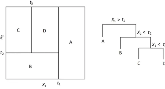
Figure 3: An example of recursive splitting with a decision tree. In the tree on the right, taking the left path in the tree means that the statement is true and taking the right means that it is false.

In Figure 3 we have four different areas with three different split criteria. So for example if we have an inputz = [z1, z2], where z1 < t1 and z2 < t2 then we will give z the classB.

Our goal is to construct the areas A1, A2, . . . , Ak in such a way that the RSS is

minimized. Recursive binary splitting is a good method of creating the decision tree. The method is top-down, it begins by having every observation in the same area, as well as greedy, only looking at the split that minimizes RSS at the current step instead of trying to base the decision on future steps.

Our data points consist of m features, so one observation is in the following form X = [x1, x2, . . . , xm]. In each step of the recursive binary splitting we choose a

feature j and a cutpoint s such that the RSS value is reduced the most when the new regions are split into the areas {X|xj < s} and {X|xj ≥s}. So for any j and

s we get two areas

A1(j, s) ={X|xj < s}and A2(j, s) = {X|xj ≥s} (18)

(18)

X i:Xi∈A1(j,s) (yi−yˆA1) 2 + X i:Xi∈A2(j,s) (yi−yˆA2) 2 . (19)

After splitting the space into the two areas we continue doing it the same way, only now we split the new smaller areas instead of the entire space. We continue doing this until some criterion is met, for example we could have a minimum amount of elements which each area should contain, stopping when there are fewer. We could also continue training until we get a low enough error rate for on our validation set. Once we have reached our stopping criteria then we check which area our observation belongs to and predict its value to be the mean of that area in a regression setting.

4.1.1 Pruning decision trees

After the decision tree is created it may work well on the training data but poorly on the test data, due to overfitting. The larger we make the tree, the more complex it becomes which leads to a bigger possibility of overfitting. One possibility of creating a suitably complex tree is by using early stopping. With early stopping we stop creating the decision tree as soon as the RSS does not decrease more than a minimum amount. This method does reduce the complexity of the tree but by stopping early we may also miss out on some splits which may have greatly reduced the RSS after our stopping point.

The alternative to early stopping is to first grow a large tree and then prune it in order to decrease the complexity. Informally pruning a tree means removing a subtree according to some heuristic. We should prune the tree and choose the subtree which has the smallest error rate. We do not, however, want to try every possible subtree, seeing as there may be a large amount of them, so instead we do weakest link pruning.

In more detail, when doing weakest link pruning we get as a result a series of trees T0, . . . , Tm. HereT0 is the original full tree andTm is simply the root node. At each

step i we remove a subtree from the previous tree Ti−1 and replace that node with a suitable value, as we did when building the tree. The subtree to be removed at each step is the one which minimizes

RSS(Ti+1)−RSS(Ti)

|Ti| − |Ti+1|

(19)

where|Tk|is the size of tree Tk. After we have our series of trees we choose the best

possible tree by cross-validating or using a validation set.

4.2 Improvements to decision trees

One problem with decision tree models is that they tend to have a high variance, meaning that even a small difference in the inputs can result in very different types of trees. In order to reduce this high variance bagging can be used. Bagging consists of first bootstrapping, that is, randomly sampling with replacement from the original training data, creatingB bootstrapped training sets of the same size as the original set. Notice that sampling with replacement means that one sample may be chosen more than once. After we have the new training sets we train B different models p1, p2, . . . , pB using the sets. When we then want to perform a prediction for one

observation x we take the mean of all of the models predictions

pbagging(x) = 1 B B X b=1 pb(x). (21)

By averaging these results we are able to reduce the variance of the model [Bre96]. Another way of enhancing regular decision trees is random forests. As with bagging, random forests also use bootstrapping to create multiple training sets out of the original one before training the trees. The difference between the two methods is that whenever we are training a random forest we pick features from a subset of features when creating splits, instead of using the entire set. The amount of features used ism and pis the count of all of the features. The set ofm features from which we choose from is randomly sampled from the full set of features. Usually the amount of features is chosen to be m ≈ √p. This set of m features is chosen for each individual tree.

This method is very good at creating trees which are different from one another. If we would have a data set which has one feature which is considerably stronger than the other ones then using bagging would most likely give us multiple trees which use that feature in the first split. This creates many similar looking trees, which are highly correlated and does not help much with reducing variance.

(20)

5 Neural networks

Neural networks are a common tool used to solve many different machine learning problems. They have been modeled on how the human brain works and can be used to solve both classification and regression problems. Neural networks are highly versatile, as well as being able to generally give highly accurate predictions with low bias. These networks usually require high amounts of data for them to be trained properly. Deep networks are also extremely unintuitive, one can not simply look at the network structure and understand what it is going to give as an output. [Mur12]

5.1 Definition

A neural network consists of nodes, or neurons, which are connected to each other in graph-like structure. The network has an input layer, output layer as well as one or more hidden layers. All of the layers can contain multiple nodes.

Figure 4: An example of a neural network [Nie15]

5.2 Forward propagation

Forward propagation is when we pass an input through our network in order to receive an output. This is done both in the learning phase as well as when we want to use our finished network to get predictions. We begin our forward pass by first calculating the activation for each our nodes. We do this by, for each node, first

(21)

multiply each of its inputs with the weight of the node and then take the sum of the resulting values. This sum is the activation value for the node. [Mur12]

When we have our activation value for each node then we apply a transfer function, or activation function, on it. For a simple perceptron, a network consisting of only one node, the activation function for the input values xj

fj(x) =    1 if P jwjxj +b >0 0 otherwise (22)

Where b is the bias, or the threshold value for the activation of the node, and wj

are the weights. Another popular activation function used is the sigmoid function which returns a real-valued output between 0 and 1 as defined by

σ(x) = 1

1 +e−x. (23)

Other activation functions which are also used are the Rectified Linear Unit (ReLu), σ(x) = max(0, x), and Tanh, σ(x) = tanh(x). Combining the calculation of the activation value and the transfer function we get a formula for the output ai

j of the

jth _{neuron in the} _ith _layer

ai_j =σ X

k

(w_jki ·ai_k−1+bi_j

. (24)

5.3 Teaching a neural network

When creating a neural network we first need to decide the layout of the network. The amount of neurons and layers is not something which we are trying to optimize, it remains static when we are teaching the network. We will also need to initialize the weights of our nodes. The weights are initialized to be random and then learned during the teaching process.

Teaching the network begins with forward propagation, which was explained here above. The main algorithm for adjusting the weights toward the correct ones is backpropagation, which we move on to after the forward propagation phase.

In order to be able to do backpropagation we need to first choose a cost, or loss, function. One cost function which is commonly used is the mean squared error as defined in equation 1. During the training phase the goal is to minimize our loss as

(22)

a function of the weights and biases. This can be done by using gradient decent. Gradient decent is an optimization algorithm which is used during backpropagation when teaching a neural network [Mur12]. We use the derivative of the activation function in order to adjust our weights and biases. We need to find such values for wandb so that our cost function is locally minimized. Backpropagation starts from the output layer. When we have calculated the error of the output layer we then iteratively calculate the errors for the hidden layers, which is done the following way

HiddenErrori =

X

j

(OutputErrorj·wij)·σ0(Outputi) (25)

where σ0 is the derivative of the activation function, assuming that the function is differentiable. So in equation 25 we are calculating the hidden error for layer i, defined asHiddenErrori. In the equation OutputErrorj is the error of nodej,wij

is the weight of nodej in layer iand Outputi is defined as the output of layeri. So

the error of a hidden layer is the sum of the errors for the neurons in the next layer multiplied by the weights connected to those neurons, multiplied by the derivative of the activation function. This error value is then used to calculate the rate of change for the weights

∆wij =Outputi·Errorj. (26)

So the change of the weight is the output of the neuron multiplied by the error of that neuron. This value will then be multiplied with the learning rate, or step size, and is subtracted from the weight

wij =wij −∆wij ·stepSize. (27)

We do this for each of our training samples, first doing forward propagation to get the prediction value for the input and then backpropagating the error and updating the weights. This is repeated either until we have performed a set amount of iterations or until the error is acceptably low.

5.4 Recurrent neural networks

Feedforward neural networks are not able to identify correlations between observa-tions, making them difficult to use for time-series. One data point in the time-series

(23)

data is dependent on previous data points, which is why the network needs to be able to have an internal memory for identifying these connections. Typical feedforward neural networks assume that all of the inputs are independent of each other, which is why a different kind of network is needed when predicting time-series. Speech recognition is one example of a problem which feedforward networks are unable to effectively solve [SOG+_13].

It is possible to use traditional neural networks when predicting sequenced data, but it requires the inputs to be preprocessed. In order to do that ne will need to add information about previous time steps to one input. For example if we have inputs x1, x2, . . . , xn we could transform them into vectors X1, X2, . . . , Xn where

Xt = [xt, xt−1, xt−2, . . . , xt−k]. This will obviously not provide the best results. Due

to the fact that one input will only contain a few of the previous inputs we will not be able to give good predictions for sequences with dependencies far into the past. An alternative solution is to use recurrent neural networks. In recurrent neural networks neurons can not only pass signals to neurons in the following layers but also to neurons in the same layer. This change in structure however means that we can not use backpropagation. Because of this a different version of the backpropagation algorithm has to be used, called backpropagation through time. Before being able to use normal backpropagation on the recurrent network we need to first unroll the network. When unrolling it we create copies of the neurons which have recurrent connections.

Figure 5: A recurrent neural network with one looped connection unrolled [Ola15]

In Figure 5 the network gets as an input xt, as feedforward networks do, as well

as the output of the previous input. This makes the output of our current input depend on previous inputs. After the network has been unrolled we can use normal

(24)

backpropagation on it. The errors are backpropagated from the final output layer to the previous layers, updating the weights as we did with regular backpropagation which can be seen in Figure 6.

Figure 6: The error backpropagated from the fourth layer [Bri15]

So recurrent networks are able to give predictions for one input based off of historical data which regular feedforward neural networks can not do. RNNs do however have some limitations in doing this. While RRNs are able to predict short term relationships well, the accuracy degrades when the distance to relevant information increases. For example when trying to predict the last word in a long document, if there is some information relevant to the word in the beginning of the document then a RNN will not be able to find that dependency. This issue is caused by the vanishing gradient problem and can be seen in the unrolled network as physical distances [Bri15].

This vanishing gradient problem occurs when backpropagating and calculating the gradient by using the chain rule. Seeing as most activation functions return results between -1 and 1 and when we use the chain rule we multiply these results the sum will decrease rapidly. This makes it difficult to optimize the parameters for the early layers of a deep network. The deeper the network the more we will multiply small numbers, making the gradient vanish. The ReLu activation function helps combat this problem, since it’s output for a valuexis max(0, x)instead of being in the range

[−1,1]. Another solution for the vanishing gradient problem is using the long short-term memory model, which is a slightly different version of the regular recurrent neural network. In the recurrence part of the long-short term memory network the activation function is an identity function with the derivative of 1, which is why the gradient does not vanish but stays constant instead. We will next explain how these networks are built.

(25)

5.4.1 Long short-term memory

Long short-term memory (LSTM) is a special kind of RNN which was first proposed by Hochreiter & Schmidhuber in 1997 [HS97]. LSTM networks are designed to work well with data which has long-term dependencies. For this reason LSTM is frequently used for solving tasks such as speech recognition, when regular RNN do not give accurate predictions.

The difference between the regular RNN networks and LSTM networks is the repeat-ing module withrepeat-ing each layer. In RNNs the module is quite simple, it concatenates the output of the previous layer with the input of the current layer and then uses an activation function on that value. A LSTM module contains quite a lot more than just a node with an activation function as seen in Figure 7 where we have one example of how a LSTM module may look.

Figure 7: A LSTM module containing four layers [Ola15]

Figure 8: A legend for the contents of Figure 7 [Ola15]

In Figure 7 every line stands for a vector which is gotten as output from one cell and given as input to some other cell. The pointwise operations are either vector multiplication or vector addition, depending on the sign inside the circle.

The central part of the LSTM module is the so called cell stateCt, which runs along

(26)

Figure 9: The cell state of the module [Ola15]

The cell state is changed by using so called gates. Gates decide if information should be added to the cell state, or if some information should be removed from the state. The module contains three gates.

The first of these three gates is a sigmoid layer and is called the forget gate layer. This gate decides what information should be disregarded from the cell state. It takes the output from the previous module ht−1 as well as xt which is our current

input and uses a sigmoid activation function on them. The sigmoid function outputs values in the range [0,1], where 0 means we leave out everything and 1 means we keep everything.

(27)

In Figure 10 the functionft is defined as

ft =σ(Wf ·[ht−1, xt] +bf), (28)

σ is the activation function,Wf is the weights for layer f and bf is the bias for layer

f. After selecting what information to remove from the cell state we need to pick what new data we need to save to the state. Saving new information to the cell state consists of two layers, a sigmoid layer called the input gate layer as well as a tanh layer. The point of theinput gate layer is to select what values need to be updated and the tanh layer creates a vector which contains values that might be added to the cell state. The results of these two layers are then put together and the result of that will be used to update the cell state.

Figure 11: Layers for selecting data that will be added to the cell state [Ola15]

it and C˜t in Figure 11 are defined as

it =σ(Wi·[ht−1, xt] +bi)

˜

Ct = tanh(WC ·[ht−1, xt] +bC).

(29) We have now calculated what needs to be removed from the cell state and what needs to be added to it. It this next step we need to do the actual updating of the cell state. We start by multiplying the previous cell stateCt−1 withft which is what

we chose to forget. After that we first multiply the values it and Cˆt and add that

(28)

Figure 12: Updating the cell state [Ola15]

Ct in Figure 12 is defined as

Ct=ft·Ct−1+it·C˜t. (30)

The last thing to calculate is the actual output corresponding to the current input. Before returning the output we first need to filter the cell state. We first pass ht−1 and xt through a sigmoid gate, this output determines what part of the cell state

should be passed as an output. We also need to pass the cell state through a tanh function to get the values to be in the range [−1,1]. We get our final output after multiplying these two results together.

(29)

In Figure 13 ot and ht are defined as

ot=σ(Wo·[ht−1, xt] +bo)

ht=ot·tanh(Ct).

(31) So herehtis the final output of the module and the prediction for the current input.

The output, along with the cell state will then be passed on to the next module.

5.4.2 Different long short-term memory variants

What was explained here was the basic version of a LSTM network, there are mul-tiple other variants which all vary slightly. Most papers which use LSTM networks deal with some sort of variant of the original version.

A common change to the normal LSTM is to add so called peephole connections. These are connections between the cell state and the gates, giving the gates informa-tion about the cell state. This version was originally created by Gers & Schmidhuber in 2000 [Sch00].

Figure 14: A LSTM module with peephole connections [Ola15]

Here in Figure 14ft, it and ot are defined as

ft=σ(Wf ·[Ct−1, ht−1, xt] +bf)

it=σ(Wi·[Ct−1, ht−1, xt] +bi)

ot=σ(Wo·[Ct, ht−1, xt] +bo).

(30)

Here above in Figure 14 we have added one peephole connection to every gate, but not all papers do this. It is also possible to only add connections to a few gates. LSTM can also be changed by connecting the forget gates with the input gates. It is done by only removing information from the cell state whenever we add something to it. The decision to forget something is made only when we decide to add something new to the state.

One drastically different, but a lot simpler, LSTM version is called the Gated Re-current Unit (GRU). Instead of having separate input and forget gates it combines them both into an update gate. It also doesn’t have a cell state, it joins the cell state with the hidden state [CvMG+_14].

Figure 15: The Gated Recurrent Unit [Ola15]

The variables in Figure 15 are defined as

zt=σ(Wz·[ht−1, xt]) rt=σ(Wr·[ht−1, xt]) ˜ ht= tanh(W ·[rt∗ht−1, xt]) ht= (1−zt)∗ht−1+zt∗h˜t. (33)

We explained here some of the more popular variants of LSTM. Greff et al. did a comparison of 8 different LSTM methods, comparing them to each other as well as to the vanilla version of LSTM [GSK+15]. They came to the conclusion that

(31)

the regular LSTM performed quite well on multiple different datasets compared to the modified versions. The variations did not have a significant improvement on the performance. They also noticed that some changes, such as coupling the input gate with the forget gate, made the model much more simple without decreasing the performance by much.

(32)

6 Predicting carbon dioxide values

As an application of the machine learning algorithms which we have discussed we present 2 case-studies, one involving regression in this chapter and one involving classification in chapter 7.

Ventilation systems usually have sensors in rooms which detect the carbon dioxide levels and activate the air conditioning when the level goes over some threshold. Our goal is to create a machine learning model which could forecast a rise in the CO2 level in a room. If we can successfully predict when the air quality will become

bad then we can preemptively turn on the air condition before the people in the room will notice.

6.1 Background

The room that was used for this study is located at Keilaranta 5, Espoo. The name of the room is HQ Tampere and it is located on the fourth floor. Inside the room we have a K-30 CO2 sensor [CO215] as well as a passive infrared (PIR) sensor which

collects motion sensor data. The motion sensors are either 311 Ceiling PIR Detectors [Hel16] or 312 Multisensors with linked PIR [Hel17]. The room has space for up 6 people and it was frequently used for meetings during the time when we collected our measurements. At our disposal we had data from both the PIR sensor and the CO2 sensor, as well as data from the lighting control panel in the room. We collected

the data for between March 20th and March 31st, only using data gathered during business days because the data gathered during weekends was rather monotone and it did not help us when training our model.

The first step was to covert the data into a format which is suitable as inputs for a learning algorithm. Originally the CO2 measurements were in the format

{timestamp : time,CO2 : CO2value}, the CO2 value at a certain time, and the

motion event data was simply {timestamp : time}, the time when a motion event was detected. The CO2 value was measured about once every two seconds, but the

value did not change drastically between measurements which is why we decided to only have one input for each minute. This did not decrease the accuracy of the model, but did however decrease the training time. So for each day we created one input and one output file. The files contain one line for each minute of the day where one row has the current CO2 value as well as a 1 if there has occurred a motion

(33)

the CO2 value Tf orward minutes in the future, which is what we will be predicting

with the models we are creating here.

6.2 Feature extraction

For machine learning models which are not good at forecasting time-series, such as random forests, we transform the inputs before training our model with it. As mentioned earlier, the input data which we have at our disposal at the start is the CO2 value as well as the motion event data.

Firstly we wanted to use the motion data to create some input features. We tried some different input feature variants, most of which are explained in the next chap-ter. The one feature which we found out to be most effective in increasing the accu-racy was the count of events between Tcurrent−Tf orward and Tcurrent. Here Tcurrent

stands for the current time andTf orward is a predetermined amount of minutes where

Tcurrent+Tf orward is the time for which we are predicting the CO2 value. So each of

our inputs will have one feature which tells us how many motion detection events have occurred in the previous Tf orward minutes. We decided to set Tf orward = 10,

because if we know that the CO2 value will begin to rise in 10 minutes we will have

time to activate the ventilation system in order to negate the rise.

Then we wanted to extract some good features by using the CO2 value. The first

set of features created using this value was the difference between the current CO2

value and earlier CO2 values. This set of feature tells us how the value has changed,

which will in turn help the model figure out how the value will change in the future. For our input vector we added a few such features

difference(Tcurrent, Tcurrent−Tf orward) and

difference Tcurrent, Tcurrent− Tf orward 2 (34)

where difference(x, y) is a function for calculating the difference in CO2 values at

time x and time y. So these two features both tell us whether the CO2 value has

been increasing or decreasing.

Our following features were received by calculating some measures on previous CO2

values. These measures are the mean, standard deviation, maximum value as well as the minimum value of the sublist

(34)

sublist(Tcurrent, Tpast) = {CO2i|Tcurrent−Tpast< Ti < Tcurrent}. (35)

The sublist function returns all of the CO2 values between times Tcurrent −Tpast

andTcurrent.This sublist contains all of the CO2 measurements for the previous Tpast

minutes. We then need to figure out the optimal value for the Tpast parameter.

We tried multiple different possibilities for this parameter, ranging from 100 all the way to 1. The value which we found out to work best for all of our test cases was Tpast = 5, which is what we will be using. So we get our features by calculating

the mean, standard deviation, maximum and minimum of sublist(Tcurrent,5). These

features give the models information about what the most common value for the CO2 measurements is as well as the deviation of the measurements.

After feature extraction we now have 8 different features to use as inputs for our models. We will next create models using these features and then compare the results.

6.3 Comparing different models

Given the input features the next step is to create machine learning models which can use these features to predict future CO2 values. It should however be noted

that these algorithms are not only limited to predicting CO2 measurements, but

any real-valued time-series, here we are only using CO2 values as one example.

Firstly we wanted to create the simplest possible model to be used as a baseline. The model we decided to use is nothing but an identity function, using the current CO2 measurement as an input and giving that same value as an output. In our case

this model can be seen as the following function

f(X) =         0 0 1 · · · 0         ·[x1, x2,· · · , xn] =xc (36)

where X is an input vector containing all features and xc is the CO2 value feature.

We will call this model the predict previous value model (PPV). This model worked surprisingly well, even outperforming some of the machine learning models. We mentioned earlier that we are using Tf orward = 10, this means that the PPV model

(35)

is predicting that the CO2 value in 10 minutes will be the same as it is currently.

This makes the PPV model lag slightly behind the actual outputs and a higher Tf orward value will increase that lag even further, making the model less accurate.

Figure 16: Visualization of the PPV model predictions

Here in Figure 16 we can see the previously mentioned lag of the PPV model when Tf orward = 10. After creating the PPV model we began creating supervised

learn-ing models. The algorithms used were linear regression (LR), decision tree (DT), random forest (RF), feedforward neural network (FFNN) and finally a long short-term memory neural network (LSTMNN). Table 1 lists the accuracy of the different models.

Table 1: Comparison of different models created for predicting CO2 values

Training RMSE Test RMSE Training R2 Score Test R2 Score

PPV 119.56 44.96 0.714 0.846 ARIMA 119.56 47.39 0.714 0.830 LR 112.77 48.77 0.659 0.786 DT 29.90 70.02 0.982 0.626 RF 43.15 54.66 0.960 0.719 FFNN 118.96 44.89 0.710 0.843 LSTMNN 24.66 9.09 0.988 0.944

(36)

In Table 1 one can notice that the training scores are worse than the test scores for some of the models, this is due to there being a large peak in the CO2 value in the

training data, which was difficult to model. This problem with the training data and the test data being so different could have been solved by using cross-validation. The first 3 machine learning models, as well as the ARIMA model, used the input features which we defined in the previous section. The two remaining models which are both neural networks only use the CO2 values as inputs, seeing as they perform

well using only the original time-series as input.

6.3.1 ARIMA model

The first model we created was an ARIMA model to see how it compared to the supervised learning methods. As with our other models, this one was created in Python. We used the Python package called statsmodels [SP10] in order to make our ARIMA model. The model which we created was a ARIMA(5,1,0) model, meaning that the lag value for autoregression is 5, the difference is of order 1 which makes the time-series stationary and the order of the moving average model is 0. When comparing to our machine learning models it performed quite well. The ARIMA model was only slightly worse than the PPV model, it beat all of the LR, DT and the RF models in accuracy. The only machine learning models which it could not outperform were the neural network models.

6.3.2 Linear regression model

The following model we created was a linear regression model. The LR model, as well as the DT and RF models, was written in Python using the scikit-learn machine learning library [PVG+_{11]. When compared to the PPV model the LR} model performed reasonably well, yet still worse than the baseline model. Both the RMSE and R2 _{scores were quite close to the PPV model scores, being only about}

8%worse which can be seen in table 1. Since the accuracy was worse than the PPV it is clear that we can not use it as our final model.

6.3.3 Decision tree and random forest models

The next two models are both based on decision trees, one being a decision tree model and the second one being a random forest model. As discussed in Chapter 4,

(37)

decision trees are not as well suited for regression tasks as classification tasks. This discussion is supported by our experiments, as seen in Table 1.

Figure 17: Comparison of the predictions of the decision tree model (left) and the random forest model (right)

In table 1 we can see that both the DT model and the RF model performed quite poorly. The DT model had a R2 score of 0.626 and the RF model had 0.719, both worse than the PPV model as well as the LR model. We can also see a visualization of how they performed in Figure 17. In the figure it is clear that the DT prediction varies highly, it slightly follows the actual CO2 value but not nearly enough to be

considered as out final model. The RF model does perform better than the DT model, as it should seeing as it is an improvement upon the DT model, yet still not well enough to outperform the PPV model. This low accuracy may mean that decision tree models are not quite good enough with regression tasks, which is why we can not use them here.

The poor performance of the decision tree models compared to the baseline is an indication of overfitting. We tried reducing the overfit by training the models by giving them only the current CO2 value as input. This did however not reduce the

(38)

6.3.4 Neural network models

The final models which we consider are neural network models, one of which is a feedforward neural network and the other one is a recurrent neural network. As with the decision tree models, the feedforward neural network (MLP) model was created using the scikit-learn library. This model performed much better than the previous ones, with a performance similar to the PPV model. But one could argue that since the results of this model are so similar to the PPV model and creating the PPV model is much simpler, there is no reason to use it over the PPV model. So as mentioned the final model that we created was a Long short-term memory (LSTM) model. This model was created using the Keras Python library [C+15], which in turn used the Tensorflow [AAB+15]. With the Keras library we were able to manually create our neural network. The network which we created was not overly complex, it contained one LSTM layer as well as one dense layer with MSE as the loss function. We can see by the very high test R2 _{score in table 1 that this} model performed extremely well, beating all of the other models with a wide margin.

Figure 18: Comparison of the predictions of the feedforward neural network model (left) and the LSTM network model (right)

Here in Figure 18 we can see a comparison of the FFNN model and the LSTM model. Both of the models seem quite similar, both follow the actual output values very closely. The one thing to note however is that the FFNN model predictions lag behind the real outputs slightly more than the LSTM model predictions do, which

(39)

is the reason why the LSTM model has better accuracy. This result is one which we expected, we discussed how the RNN networks is good at discovering patterns in time-series data and here we can see how it works in practice.

6.4 Applying the best model

After comparing the different models for predicting the CO2 time-series data we

found one which was better than the others. Our baseline model was quite good, considering how simple it was. It did however become increasingly less accurate when we tried making predictions further into the future, which is why it could not be used in our final application. The linear regression model was nearly as good as the baseline model, without the increased accuracy loss. If we are looking to make predictions more than 30 minutes into the future, then choosing the LR model over the PPV model would be the correct choice.

Both of the models based on decision trees were quite inaccurate. The decision tree model varied highly, making the predictions quite imprecise. The random forest model was slightly better, with a bit less of variance, it was still not better than the PPV or the LR model which is why these models can not be used in our final application.

Lastly we had the neural network models, both of which performed very well. The traditional feedforward neural network model had an accuracy more or less equal to that of the PPV model, without the PPV models apparent flaw, making it a good model option for us to use. Although the FFNN model had good accuracy it was still far worse than the best model that we tried out, the long short-term memory neural network model. This model was the clear winner in terms of accuracy, which is why it is the one we will use in our application.

We used the LSTM model to create an application which creates a new model from the training data daily and constantly gets new data from the sensors. This applica-tion is then be called when a user wants a CO2prediction. It is then also possible for

other applications to use these predictions. An application which controls the venti-lation system can for example constantly call our model for predictions in order for it to know how to adjust the ventilation for each room. By doing this the ventilation system responds faster to the changes in the CO2 level, which hopefully means that

the people in the room in question will not notice a decrease in air quality before the ventilation system turns on. This will then in turn make it more pleasant for

(40)

(41)

7 Predicting lighting events based on motion sensor

data

It is common for a building lighting system to have some motion detection sensors along with the lights. These motion sensors are often used to activate the lighting system, having some particular sensors coupled with a group of luminaires. At the Helvar office in Espoo the data collected by the PIR sensors are also saved in a database. With this data at our disposal it could be possible to predict whether or not a sensor will see movement within a certain period of time. It would be beneficial to be able to predict the activity of one PIR sensor, that way we can know beforehand when a light will be activated and can turn it on preemptively.

7.1 Background

So our goal is to create a machine learning model which can make predictions based on the data collected by the motion sensors. The model will take as an input the motion data for one sensor and output the probability that the sensor will see movement in n minutes. The raw input data is an array of timestamps, where a timestamp means that the sensor has detected movement at that time. This format of data is of course not ideal when making time-series predictions, and we will have to change it before feeding it to some machine learning model. The first step is to transform the data from the format seen in Equation 37 into a time-series.

["00:00 01.01.2017","00:02 01.01.2017","00:05 01.01.2017", ...] (37) We transform array of timestamps so that we have one binary digit for each minute. If the value is 0 then there has not been a motion event during that minute and if it is a 1 then there has been an event. So the data above would look like this when transformed

[1,0,1,0,0,1, ...] (38) From now on we assume that all data to be in this form. For one building there are multiple motion sensors and for each of them we have one binary vector indicating activity for a certain period of time.

(42)

7.2 Feature extraction

The binary data which we now have is not quite ideal for making predictions. A binary vector does not contain much information for making accurate predictions. We will here discuss a few different features which we can extract from the data and see which of them would be the most useful. The features will hopefully give us more information about the current state of the sensor in question.

7.2.1 Time since previous events

The first set of features which we will use is where we change one data point from a binary value to be a vector of length previousEventCount. Here the element k in this vector stands for the amount of minutes since the kth motion detection. So at time Tcurrent we could have the following input

[2,10,23] (39) This input means that the previous motion detection for the sensor was 2 minutes ago, the event before that was 10 minutes ago and the event before that was 23 before time Tcurrent. This list will be referred to as timeSincePreviousEvents. Here

we have set previousEventCount = 3. So the input vector will consist of multiple vectors of length previousEventCount, having one vector for each minute, which could look something similar to this

[...,[2,10,23],[0,3,11],[1,4,12], ...] (40) This feature adds a notion of memory to the data, instead of just having one binary value per minute one now knows when the earlier events occurred. This helps teaching models which do not have any internal memory, as such models would otherwise have trouble.

We tried different previousEventCount values, trying to determine the one which one gives us the best performance. The values which we tried were 1, 3, 5, 10, 25 and 50. What we noticed was that increasing previousEventCount often led to improved performance, even if some exceptions were observed with some datasets. This result is as expected, the more information we have about the previous events the better. So in the end we decided to use previousEventCount= 25, due to this value working well in our testing.

(43)

7.2.2 Amount of events during previous Tback minutes

The second alternative for formatting resembles the first. We want to add informa-tion about the previous events into the data here as well. With this version of the data we will transform one binary value in the input array into a integer which is the amount of events in the previous Tback minutes. For each time step we will use

a function for getting this event count

amountOfEvents=eventCount(Tcurrent−Tback, Tcurrent) (41)

Where eventCount(x, y) is a function which calculates the amount of motion detec-tion event between time x and time y. Tcurrent is simply the time at the current

time step. So when we are given the following input vector

[1,0,1,0,0,1,0,0] (42) it will be transformed into the following vector when the binary value at each time step is changed to be the returned value of the eventCount function, whenTback = 3

[1,1,2,2,1,2,1,1] (43) Having the data in this form will better display when there is a large amount of activity and when the sensor does not notice much movement. When a sensor is in an area without much traffic it means that the data will be quite sparse. The data will mostly contain zeroes, making it even more difficult to make predictions using the binary data. This data format helps with the sparsity in the data by reducing the amount of zeroes in the input.

We will also add some features which are similar to the previous one. These features will also be taken from from the eventCount function but the time period will be slightly different. These time periods will be gotten with the eventCount function in the following way

eventsDDaysAgo(D) = eventCount(Tcurrent−D,

Tcurrent−D+Tf orward)

(44)

where D is the number of days and Tf orward an amount of minutes. The Tf orward

(44)

willEventOccur(Tcurrent, Tf orward) =          1, if eventCount(Tcurrent, Tcurrent+Tf orward)>= 1 0, otherwise (45)

So the Tf orward value is determined by how far in the future we want to make our

prediction. The idea with the eventCountDDaysAgo features is that a sensor often sees similar events at the same time of day. If we for example want to predict whether there will be a motion event for a sensor in the next 10 minutes, Tf orward

= 10, then the eventCountDDaysAgo value will be the amount of events for the next 10 minutes D days ago. We could for example use features where D ∈ [1,7], which would give us two features which tell us how many events there were for the predicted period yesterday as well as a week ago. The hope with these features is that knowing how active the sensor has been during the period to be predicted the model can more easily make the predictions.

As with the previousEventCount value we also tested different values for Tback to

figure out which one would work the best. We noticed the same thing as with the previousEventCount value, an increase in the value improved the performance. Here we tried the following values 5, 10, 25, 60 and 120. The value which worked the best for all datasets was 60, which is why we chose to use it.

7.2.3 Weekday feature and Tf orward features

The final features which we will add to our inputs are slightly simpler than the previous ones. The first of which is a binary value indicating whether or not the current time step is a weekday. We will use a function which returns the following values isWeekday(Tcurrent) =    1, if Tcurrent is a weekday 0, otherwise (46) We also decided to include the Tf orward value as a feature. This was done to give

the model information about how many minutes in the future our predictions are made.

The difference betweenTf orward and our other parameters is that it is not something

(45)

in the future we want to predict for, on what we want to use the predictions for. Since the probability of an event occurring increases the longer time goes on then the accuracy of our model will also increase when the value of Tf orward grows. In

other words trying to predict if an event will happen during the next minute will be more difficult than predicting for the next 10 minutes.

7.2.4 Final input vector

We now have the input features which we will use while training our model as well as our outputs. The full input vector for one sensor will be the following

           timeSincePreviousEvents eventCount(Tcurrent - Tback, Tcurrent)

eventsDDaysAgo(T1day) eventsDDaysAgo(T7days) isWeekday(Tcurrent) Tf orward            (47)

while the matching output it simply the value returned by the willEventOccur func-tion.

The vector 47 is the input for one time step for one sensor after we have parsed the raw data. With these features we have information about how long it has been since the previous events occurred, how many events there have been in the previous Tback minutes as well as how many events have happened during the period to be

predicted yesterday and a week ago. We also have features which tell us whether or not the current timestep is a weekday and finally the value of Tf orward. With

these features we hope to be able to create a model which can accurately predict the future events for one sensor.

7.3 Creating the model

We have now decided what features the input vector will contain, as seen in vector 47, for a single sensor. We however have data from multiple sensors available to us. Here below we can see the floorplan of the Helvar office at Keilaranta 5, Espoo. Each red box marks the location of a sensor with the device id of the sensor written in white.

(46)

We picked two different sensors which we tried to make predictions for, firstly the one with the id4.2.56which is in the social kitchen and secondly the one in the open office that has the id 7.1.59. Both of them are in high traffic areas, meaning that there will be much data from the sensors to work with. They are also surrounded by many other sensors which also prove to be useful when training our model.

Figure 19: All of the sensors located in the Helvar office in Espoo

The model we decided to use as a baseline was a linear classification model. The model was created using the Apache Spark Python API (PySpark) Machine Learning Library (MLlib). The code was run on an Amazon EC2 cluster.

The next thing we want to do is figure out is how many of the sensors we want to use as input when we are training our model. We tried multiple different options when training the model. The first option is the simplest one, to only use our output sensor as an input. This way the model does not get any knowledge about the other sensors. Having only the output sensor as our input means that we will have less data overall, making the creation of the model faster since we do not need to fetch

(47)

as much data.

The second idea we had was to use sensors which are nearby the predicted sen-sor as input. By giving nearby sensen-sors as inputs the model should start to inter-pret movement seen by those sensors as a sign that the sensor to be predicted will also see movement. For the social kitchen sensor we also gave the follow-ing sensors as inputs [4.2.60,4.2.57,4.1.61,4.2.62] and for the open office one these

[7.1.57,7.1.61,7.2.59,7.2.60].

We also decided to test adding many seemingly random sensors as inputs, ones which were not near the sensor for which we want to make our predictions. We tried this to see if this would improve the accuracy of the models. In addition to the previous lists of sensor, which were all near the sensor in question, we also added many which were scattered all over the office. In total we added around 20 sensors to our inputs. Due to us having so many sensors as inputs here it also took much longer for us to create the models, the large amount of data makes running our program take a lot longer.

We tried all of these different input sets, creating a linear prediction model for all of them. We came to the conclusion that the difference was not significant, using only one sensor as the input was marginally better for the majority of our test cases. Seeing as there was not much of a difference we decided to simply use one sensor as the input, since it also decreased the run time when creating the models.

7.4 Comparing different models

When testing the performance of the different models we used a linear classifier as a simple baseline. Here we want to see how other models compare to it so that we can choose the most accurate model to be used in our application for predicting motion events. We used the same kinds of algorithms as in the previous chapter, linear regression (LR), decision tree (DT), random forest (RF), feedforward neural network (FFNN) and finally long short-term memory neural network (LSTMNN). Here in table 2 we can see the comparison between the different algorithms. The classes here are 0 or 1, where 0 means that an event will not occur and 1 means that it will. We are showing the measures for the classes separately to make it clear that predicting when an event occurs is more difficult for the models than predicting class 0 is. This is due to the fact that class 0 is the more common one in our dataset, it is less likely that a sensor sees movement. The f1-score is the one we want to focus

Predicting building-automation time-series data with supervised methods