Algorithm Selection on Data Streams
Jan N. van Rijn1, Geoffrey Holmes2,Bernhard Pfahringer2, and Joaquin Vanschoren3 1
Leiden University, Leiden, Netherlands, [email protected]
2 University of Waikato, Hamilton, New Zealand,
{geoff,bernhard}@cs.waikato.ac.nz
3 Eindhoven University of Technology, Eindhoven, Netherlands,
Abstract. We explore the possibilities of meta-learning on data streams,
in particular algorithm selection. In a first experiment we calculate the characteristics of a small sample of a data stream, and try to predict which classifier performs best on the entire stream. This yields promis-ing results and interestpromis-ing patterns. In a second experiment, we build a meta-classifier that predicts, based on measurable data characteristics in a window of the data stream, the best classifier for the next window. The results show that this meta-algorithm is very competitive with state of the art ensembles, such as OzaBag, OzaBoost and Leveraged Bagging. The results of all experiments are made publicly available in an online experiment database, for the purpose of verifiability, reproducibility and generalizability.
Keywords: Meta Learning, Data Stream Mining
1
Introduction
Modern society produces vast amounts of data coming, for instance, from sensor networks and various text sources on the internet. Various machine learning algorithms are able to capture general trends and make predictions for future observations with a reasonable success rate. The number of algorithms is large, and most of these work well on a varying range of data streams. However, there is not much knowledge yet about on which kinds of data certain algorithms perform well and when a certain algorithm should be preferred over another.
In this work we investigate how to predict what algorithm will perform well on a given data stream. This problem is generally known as the algorithm selection problem [14]. For each data stream, we measure the performance of various data stream classifiers and we calculate measurable data characteristics, called meta-features. In addition to many existing meta-features, we introduce a new type of meta-feature, based on concept drift detection methods. Next, we build a model that predicts which algorithms will work well on a given data stream based on its characteristics. Indeed, having knowledge about which classifier to apply on what data could greatly increase the performance of predictive tools in
real world applications. For example, it is common for the performance curves of data stream algorithms to cross as the stream evolves. This means that at certain points in the stream, the data is best modelled with algorithm A, while at a later point, the data is better modelled with algorithm B. As such, selecting the right algorithm at each point in the stream has the potential to increase performance. In this work we focus on data streams with a nominal target. Although much work has been done on both data streams and meta-learning, to the best of our knowledge, this is the first effort to do meta-learning on data streams.
The remainder of this paper is structured as follows. Section 2 contains a de-scription of related work. Section 3 describes how the meta-dataset was created, the data streams that it contains, how they are characterized, and how we have measured the performance of data stream algorithms. Section 4 describes an experiment in which we calculate the characteristics of asmall sampleof a data stream, and predict which classifier performs best on the entire stream. Next, Section 5 describes a second experiment, in which we continuously measure the characteristics of asliding windowon the data stream, and use a meta-algorithm to predict the best classifier for the next window. In Section 6 we present and discuss some emerging patterns from the data. Section 7 concludes.
2
Related Work
It has been recognized that mining data streams differs from conventional batch data mining [4, 13]. In the conventional batch setting, usually a limited amount of data is provided and the goal is to build a model that fits the data as well as possible, whereas in the data stream setting, there is a possibly infinite amount of data, with concepts possibly changing over time, and the goal is to build a model that captures general trends.
More specifically, the requirements for processing streams of data are: process one example at a time (and inspect it only once), use a limited amount of time and memory, and be ready to predict at any point in the stream [3, 13]. These re-quirements inhibit the use of most batch data mining algorithms. However, some algorithms can trivially be used or adapted to be used in a data stream setting, for example, NaiveBayes, k Nearest Neighbour, and Stochastic Gradient Descent, as done in [13]. Also, many algorithms have been created specifically to operate on data streams. Most notably, theHoeffding Tree[6] is a tree based algorithm that splits based on information gain, but using only a small sample of the data determined by the Hoeffding bound. The Hoeffding bound gives an upper bound on the difference between the mean of a variable estimated after a number of observations and the true mean, with a certain probability.
Conventional batch data mining methods can also be adapted for use in the data streams setting by training them on a set of instances sampled from recent data. Typically, a set of w(window size) training instances is formed. Every w instances form a batch and are provided to the learner, which builds a model based on these instances. The disadvantages of this approach are that the most recent examples are not used until a batch is complete, and old models need to
be deleted to make room for new models. Read et al. [13] distinguish between instance incremental methods and batch incremental methods and compare the performance of both approaches. Their main conclusion is that the performance in terms of accuracy is equivalent. However, the instance incremental algorithms use fewer resources.
Ensembles of classifiers are among the best performing learning algorithms in the traditional batch setting. Multiple models are produced that all vote for the label of a certain instance. The final prediction is made according to a predefined voting schema, e.g., the class with the most votes wins. In [10] it is proven that the error rate of an ensemble in the limit goes to zero if two conditions are met: first, the individual models must do better than random guessing, and second, the individual models must be diverse, meaning that their errors should not be correlated. Popular ensemble methods in the traditional batch setting are Bag-ging [5], Boosting [17] and Stacking [7]. BagBag-ging and Boosting have equivalents in the data stream setting, e.g., OzaBag [11], OzaBoost [11] and Leveraging Bag-ging [4]. The Average Weighted Ensemble [20] tracks which individual classifiers perform well on recent data, and uses this information to weight the votes.
The field of meta-learning addresses the question what machine learning algorithms work well on what data. The algorithm selection problem, formalised by Rice in [14], is a natural problem from the field of meta-learning. According to the definition of Rice, the problem spaceP consists of all machine learning tasks from a certain domain, the feature spaceF contains measurable characteristics calculated upon this data (called meta-features), the algorithm spaceAis the set of all considered algorithms that can execute these tasks and the performance space Y represents the mapping of these algorithms to a set of performance measures. The task is for any given x∈P, to select the algorithm α∈Athat maximizes a predefined performance measure y ∈ Y, which is a classification problem. Similar ranking and regression problems are derived from this.
Much effort has been devoted to the development of meta-features that effec-tively describe the characteristics of the data (called meta-features). Commonly used meta-features are typically categorised as one of the following: simple (num-ber of instances, num(num-ber of attributes, num(num-ber of classes), statistical (mean standard deviation of attributes, mean kurtosis of attributes, mean skewness of attributes), information theoretic (class entropy, mean entropy of attributes, noise-signal ratio) or landmarkers [12] (performance of a simple classifier on the data). The authors of [18] give an extensive description of many meta-features. Furthermore, they propose a new type of meta-feature, pair-wise meta-rules.
Another recent development is the concept of experiment databases [15, 19], databases which contain detailed information about a large range of experiments. Experiment databases enable the reproduction of earlier results for verification and reusability purposes, and make much larger studies (covering more algo-rithms and parameter settings) feasible [19]. Above all, experiment databases allow a variety of studies to be executed by a database look-up, rather than setting up new experiments. An example of such an online experiment database is OpenML [15].
3
Meta-dataset
For the purpose of meta-learning, we need to obtain data on previous experi-ments, i.e., runs of various algorithms on various data streams (from here on referred to asbase datasets, orbase data streams). From this we construct a so-called meta-dataset, in which each instance is a data stream characterized by a number of measurable characteristics, themeta-features, as well as performance scores of various machine learning algorithms.
3.1 Bayesian Network Generator
Unfortunately, the data stream literature contains few publicly available data streams. In order to obtain a reasonable number of experiments on data streams, we propose a new type of data generator that generates data streams based on real world data [16]. It takes a dataset as input, preferably consisting of real world data and a reasonable number of features, and builds a Bayesian Network over it, which is then used to generate instances based on the probability tables. These streams can also be combined together to simulate concept drift, similar to what is commonly done with the Covertype, Pokerhand and Electricity dataset [4].
The generator takes a dataset as input, and outputs a data stream containing a similar concept, with a predefined number of instances. The input dataset is preprocessed with the following operations: all missing values are first replaced by the majority value of that attribute, and numeric attributes are discretized using Weka’s binning algorithm [9]. Values for attributes that are numeric in the original dataset can be determined using two strategies. The nominal strategy assigns one of the bins as the attribute value, determining the bin based on the probability tables. Thenumeric strategy takes the bin with the highest proba-bility value and draws a number from this bin based on its normal distribution. The generated data streams are denoted as BNG(data,strategy,num instances), with data denoting the original dataset, strategy denoting the chosen strategy for numeric values, and instances denoting the number of generated instances. The algorithm is implemented in the OpenML MOA package4.
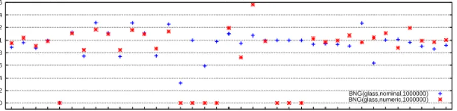
Figure 1 shows the meta-features as calculated over the two Bayesian Network Generated data streams based on theglass dataset, compared to the values of the original dataset. As many of these qualities are quite similar, there is some indication that there is a similar concept underlying the data. Thedimensionality indicates the ratio between the number of instances and the number of attributes. The decrease of this value can be explained by the fact that the number of attributes is the same, yet the number of instances has increased. Furthermore, data streams generated using the nominal strategy do not have any numeric attributes, hence meta-features likeMean Skewness Of Numeric Attributes and Mean StDev Of Numeric Attributes are zero. The meta-features indicating the J48 landmarkers (with varying confidence factors) have better values on the generated data streams, hinting at a slightly easier concept represented by the data. Similar patterns can be found for other generated data streams.
4
0 0.2 0.4 0.6 0.8 1 1.2 1.4 1.6
DecisionStumpAUCDecisionStumpErrRateDecisionStumpKappaDefaultAccuracyDimensionalityJ48.00001.AUCJ48.00001.ErrRateJ48.00001.kappaJ48.0001.AUCJ48.0001.ErrRateJ48.0001.kappaJ48.001.AUCJ48.001.ErrRateJ48.001.kappaMeanKurtosisOfNumericAttsMeanMeansOfNumericAttsMeanSkewnessOfNumericAttsMeanStdDevOfNumericAttsNBAUCNBErrRateNBKappaNegativePercentageNumNumericAttsNumberOfNumericFeaturesPercentageOfNumericAttsREPTreeDepth1AUCREPTreeDepth1ErrRateREPTreeDepth1KappaREPTreeDepth2AUCREPTreeDepth2ErrRateREPTreeDepth2KappaREPTreeDepth3AUCREPTreeDepth3ErrRateREPTreeDepth3KappaRandomTreeDepth1AUC
K=0 RandomTreeDepth2AUC K=0 RandomTreeDepth3AUC K=0 accuracy(k-NN)-accuracy(LB-kNN) BNG(glass,nominal,1000000) BNG(glass,numeric,1000000)
Fig. 1. Meta-features of two Bayesian Network Generated data streams, where each
value is divided by the corresponding meta-feature value of the original dataset.
3.2 Base data streams
The data streams generated by the Bayesian Network Generator form the basis of our meta-dataset. We took datasets from the UCI repository [1] as input for the Bayesian Network generator. We aimed to generate data streams of 1,000,000 instances, or less if the original dataset did not have enough attributes to obtain a million different instances. We used both the nominal and the numeric strategy in those cases where the original dataset had numeric attributes. In addition to these, we also generate data streams by commonly used data generators from the literature. We used the following data generators, as implemented in the MOA workbench [3]: the SEA Concepts Generator, Rotating Hyperplane Generator, Random RBF Generator and the LED Generator. For the generation of these data streams we used the same parameters as described in [13].
Additionally, we also included the commonly used datasets Covertype, Elec-tricity and Pokerhand, and a combination of these in order to generate concept drift, as is done in [4]. We also included large text datasets, i.e., the IMDB dataset and the 20 Newsgroups dataset. We converted the IMDB dataset into a binary classification problem, having the drama genre as target. The 20 News-groups dataset is first converted into 20 binary classification problems (one for every Newsgroup) and then appended again into one big binary-class dataset, as is done in [13]. This simulates a data stream with 19 concept drifts.
3.3 Meta-features
We have characterized the base data streams using a wide variety of meta-features. Most of the features are already described in the literature, e.g., in [18], and are either of the type simple, statistical, information theoretic or landmarker. We also introduce stream specific meta-features, based on a change detector. We have run bothHoeffding TreesandNaiveBayes with both theADWIN [2] and DDM [8] change detectors over all data streams, and have recorded the number
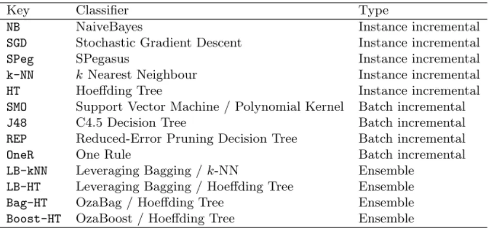
Table 1. Algorithms used in the experiments. Batch incremental classifiers have a window of size 1,000; ensembles contain 10 base classifiers;k-NNis used withk= 10.
Key Classifier Type
NB NaiveBayes Instance incremental
SGD Stochastic Gradient Descent Instance incremental
SPeg SPegasus Instance incremental
k-NN kNearest Neighbour Instance incremental
HT Hoeffding Tree Instance incremental
SMO Support Vector Machine / Polynomial Kernel Batch incremental J48 C4.5 Decision Tree Batch incremental REP Reduced-Error Pruning Decision Tree Batch incremental
OneR One Rule Batch incremental
LB-kNN Leveraging Bagging /k-NN Ensemble LB-HT Leveraging Bagging / Hoeffding Tree Ensemble
Bag-HT OzaBag / Hoeffding Tree Ensemble
Boost-HT OzaBoost / Hoeffding Tree Ensemble
of changes detected (both ADWIN and DDM) and the number of warnings (DDM only). All these meta-features are calculated for each window of 1,000 instances on each data stream.
3.4 Algorithms
The algorithms included in this study are shown in Table 1, and can be grouped into three types: instance incremental classifiers, batch incremental classifiers and ensembles. For all classifiers, we have recorded the predictive accuracy, the runtime, and RAM Hours on each data stream. The predictive accuracy was de-termined using the Interleaved Test Then Train procedure, where each instance is first used as a test instance, before it can be used to train the classifier.
4
Algorithm Selection in the Classical Setting
In the classical setting of the algorithm selection problem, the goal is to predict, for a certain dataset, what algorithm would perform best.
4.1 Experimental Setup
In prior studies, the algorithm selection problem was treated as either a clas-sification problem, regression problem, or ranking problem [18]. To investigate what kind of information can be obtained from the data, we treat the algorithm prediction problem on data streams as a classification problem. We create a meta-dataset5using the experimental data described in Section 3. For each base
5
All meta-datasets that were created for this study can be obtained from http://www.openml.org/d/
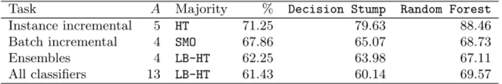
Table 2.Results of the algorithm selection problems in the classical setting. Task A Majority % Decision Stump Random Forest Instance incremental 5 HT 71.25 79.63 88.46 Batch incremental 4 SMO 67.86 65.07 68.73 Ensembles 4 LB-HT 62.25 63.98 67.11 All classifiers 13 LB-HT 61.43 60.14 69.57
data stream, the meta-features are recorded in the first window of 1,000 obser-vations. By the definition of Rice [14], this means that we are working on the algorithm selection problem with A= 13 (algorithms),P = 75 (data streams), Y =predictive accuracy (performance measure) andF= 58 (meta-features).
The goal is to predict which algorithm performs best, measured over the whole data stream. In order to obtain deeper insight into what kind of tar-gets we can predict, we also defined three sub tasks, i.e., predicting the best instance incremental classifier (A = 5), predicting the best batch incremental classifier (A= 4) and predicting the best ensemble (A= 4). We have selected the “Decision Stump” and “Random Forest” classifiers (as implemented in Weka 3.7.11 [9]) as meta-algorithms. TheRandom Forestalgorithm has proven to be a useful meta-algorithm in prior work [18], while models obtained from a single decision tree or stump are especially easy to interpret. Both classifiers are tree-based, which guards them against modeling irrelevant features. We ran the Random Forest algorithm with 100 trees and 10 attributes. We estimate the per-formance of the meta-algorithm by doing 10 times 10 fold cross-validation, and compare its performance against predicting the majority class. For each meta-dataset, we have filtered out the instances that contain a unique class value; since they will either only appear in the training or test set, these do not form a reliable source for estimating the accuracy.
4.2 Results
Table 2 shows the results obtained from the various tasks. It shows for every task which classifier performs best in most cases (and therefore is the major-ity class of the task) and in what percentage of the data streams that is the case. Column “A” denotes the number of classes that were distinguished in the tasks; column “Majority” and “%” denote the majority class and its size. The other columns denote the accuracy score of the respective meta-algorithms. TheRandom Forestalgorithm performs better than the baseline on all defined tasks. TheDecision Stumpalgorithm performs well only at predicting both the best instance incremental classifiers and ensembles. The results of both meta-algorithms on the task of predicting the best instance incremental were marked as significantly better than predicting majority class, tested using a Paired T-Test with a confidence of 95%. Since the data characteristics were obtained over only the first 1,000 instances of each stream, algorithm selection on data streams can improve results of classifiers at already very low computational cost.
5
Algorithm Selection in the Stream Setting
In data stream prediction, it is common for performance curves of different algorithms to cross each other multiple times. Whereas, at a certain interval of the stream, one of the algorithms performs best, this might be different for other intervals of the stream. By applying algorithm selection in a stream setting, our goal is to predict what algorithm will perform best for the next window of data.
5.1 Experimental Setup
In this experiment we want to determine whether meta-knowledge can improve the predictive performance of data stream algorithms in the following setting. Consider an ensemble of algorithms that are all trained on the same data stream. For each window of size w, an abstract meta-algorithm determines which al-gorithm will be used to predict the next window of instances, based on data characteristics measured in the previous window and the meta-knowledge. Note that the performance of the meta-algorithm depends on the size of this win-dow. Meta-features calculated over a small window size are probably not able to adequately represent the characteristics of the data, whereas calculating meta-features over large windows is computationally expensive. Since our previous experiment obtained good results with a window size of 1,000, we perform our experiments with the same window size.
We have constructed a new meta-dataset, containing for each window the meta-features measured over the previous interval, and the performance of all base-classifiers trained on the entire data stream up to that window. We only include a subset of the generated data streams. Indeed, since the Bayesian Net-work Generator was used to generate multiple data streams based upon the same source data (using the nominal strategy and the numeric strategy), it is likely that these data streams contain a similar concept. We therefore remove all data streams generated using the nominal strategy, if a version generated by the nu-meric strategy also exists. After filtering out these data streams, there are still 49 data streams left. The meta-dataset consists of roughly 45,000 instances, each describing a window of 1,000 observations from one of these base data streams. For each of the base data streams, a meta-algorithm is trained using only the intervals of the other data streams. We use a Random Forest (100 trees, 10 attributes) as meta-algorithm, since it proved to be a reasonable choice in the previous experiment. We measure how it performs on the meta-learning task of predicting the right algorithm for a given interval, as well as how it would actually perform on the base data streams. To the best of our knowl-edge, Leveraged Bagging Hoeffding Trees is the state of the art algorithm on these data streams, so we will compare it against our abstract algorithm. As in the previous experiment, we distinguish the tasks of selecting the best instance incremental classifier, the best batch incremental classifier and the best ensemble.
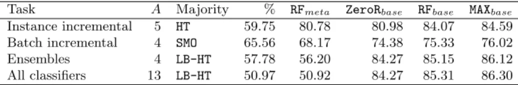
Table 3.Results of the algorithm selection problems in the stream setting.
Task A Majority % RFmeta ZeroRbase RFbase MAXbase Instance incremental 5 HT 59.75 80.78 80.98 84.07 84.59 Batch incremental 4 SMO 65.56 68.17 74.38 75.33 76.02 Ensembles 4 LB-HT 57.78 56.20 84.27 85.15 86.12 All classifiers 13 LB-HT 50.97 50.92 84.27 85.31 86.30
5.2 Results
Table 3 shows the results obtained from this experiment. As with the results of the previous experiment, column A indicates the number of classes in the classification problem, “Majority” denotes which classifier is the majority class (i.e., the classifier that performs best in most observations), and “%” shows the size of the majority class. We measure two types of accuracy,meta-level accu-racy andbase-level accuracy. Meta-level accuracy records the performance using a zero-one loss function. Consequently, it indicates for how many windows the meta-algorithm predicted the best classifier. Column RFmeta shows the
meta-level accuracy of a Random Forest. Base-meta-level accuracy records the performance using a loss function equivalent to the performance of the predicted classifier. For example, when the meta-algorithm predicts k-NN to be the best classifier on a certain interval, the accuracy ofk-NNon this interval will be used as loss. Accord-ingly, base-level accuracy indicates the performance of the meta-classifier on the base data streams when dynamically selecting the base-classifier. The base-level score of the Random Forest meta-algorithm is shown in columnRFbase. Column
ZeroRbase shows the base-level accuracy when the majority class is always
pre-dicted. Note that this is the score obtained by the majority class base-classifier, measured over all base data streams. ColumnMAXbase shows what the base-level
score would be, if for any interval the best classifier would have been predicted. As in the classical setting, it appears that determining the best instance-incremental classifier yields good results. In more than 80% of the cases, the correct classifier is predicted. This also results in a notable increase in base level performance, in such a way that it is comparable withLeveraged Bagged Hoeffding Trees(84.27), and outperforms the scores obtained byOzaBag(82.58) and OzaBoost (80.55). The results also show a consistent increase in perfor-mance. For all defined tasks, the meta-algorithm outperforms the use of the single best classifier in its pool, even though, on the ensemble task, RFmeta
performs no better than predicting the majority class. Apparently, the meta-algorithm was able to avoid the use of Leveraged Bagged Hoeffding Trees on windows where the performance is very low. Furthermore, the base level per-formances are in many cases close to the maximum possible value given the pool of classifiers. This indicates that the main challenge is to find ways to improve this limit. This could be done by using a larger set of algorithms, or by using other techniques such as parameter optimisation.
-0.008 -0.007 -0.006 -0.005 -0.004 -0.003 -0.002 -0.001 0 0.001 0.002
pokerhand-normalizedCovPokElecBNG(mfeat-fourier,numeric,1000000)20 newsgroups.drift.arff
BNG(sonar,nominal,1000000)BNG(sonar,numeric,1000000)covertypeBNG(letter,numeric,1000000)BNG(mfeat-karhunen,numeric,1000000)BNG(kr-vs-kp,nominal,1000000)electricity-normalizedBNG(mfeat-karhunen,nominal,1000000)BNG(vehicle,numeric,1000000)Hyperplane(10;0.0001)BNG(autos,numeric,1000000)BNG(letter,nominal,1000000)BNG(waveform-5000,nominal,1000000)Hyperplane(10;0.001)BNG(credit-g,nominal,1000000)BNG(mfeat-fourier,nominal,1000000)BNG(optdigits,nominal,1000000)BNG(credit-g,numeric,1000000)BNG(lymph,nominal,1000000)BNG(autos,nominal,1000000)BNG(heart-c,nominal,1000000)BNG(pendigits,nominal,1000000)BNG(lymph,numeric,1000000)BNG(pendigits,numeric,1000000)BNG(heart-statlog,nominal,1000000)BNG(vehicle,nominal,1000000)LED(50000)BNG(heart-c,numeric,1000000)BNG(heart-statlog,numeric,1000000)BNG(breast-cancer,nominal,1000000)SEA(50000)BNG(heart-h,nominal,1000000)BNG(anneal.ORIG,numeric,1000000)BNG(vowel,nominal,1000000)BNG(dermatology,numeric,1000000)SEA(50)BNG(dermatology,nominal,1000000)BNG(mfeat-zernike,numeric,1000000)IMDB.dramaBNG(anneal.ORIG,nominal,1000000)RandomRBF(50;0.0001)BNG(vowel,numeric,1000000)BNG(page-blocks,nominal,295245)BNG(page-blocks,numeric,295245)RandomRBF(10;0.001)BNG(spambase,nominal,1000000)BNG(anneal,numeric,1000000)RandomRBF(10;0.0001)RandomRBF(0;0)BNG(mfeat-zernike,nominal,1000000)BNG(anneal,nominal,1000000)covertype-normalizedBNG(hypothyroid,nominal,1000000)BNG(soybean,nominal,1000000)BNG(sick,nominal,1000000)BNG(mushroom,nominal,1000000)BNG(cmc,nominal,55296)RandomRBF(50;0.001)BNG(waveform-5000,numeric,1000000)BNG(waveform-5000,numeric,1000000)BNG(trains,nominal,1000000)BNG(vote,nominal,131072)BNG(credit-a,nominal,1000000)BNG(labor,nominal,1000000)BNG(credit-a,numeric,1000000)BNG(cmc,numeric,55296)BNG(segment,nominal,1000000)BNG(hepatitis,numeric,1000000)BNG(labor,numeric,1000000)BNG(labor,numeric,1000000)BNG(hepatitis,nominal,1000000)BNG(ionosphere,nominal,1000000)
Percentage
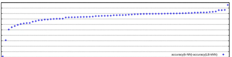
accuracy(k-NN)-accuracy(LB-kNN)
Fig. 2.The difference in predictive accuracy of k-NNand Leveraged Bagging k-NN.
(k= 10, 10 base classifiers)
6
Discoveries
In this section we discuss interesting patterns that were obtained while analysing the meta-datasets, some of which corroborate earlier findings in the literature. Other findings will form the basis of our future work.
Discovery 1 An abstract meta-classifier consisting of 5 instance incremental clas-sifiers (NaiveBayes, 10 Nearest Neighbour, SPegasus, SGDand a Hoeffding Tree) is competitive with state of the art ensembles, tested over a large range of data streams. It is likely that this result generalizes to an even larger num-ber of data streams, because both conditions for an ensemble of classifiers to be successful are met [10]: the base classifiers are diverse and do better than ran-dom guessing. Moreover, the experiment in Section 4 shows that it is possible to predict which one will perform well based on prior data.
Discovery 2 In contrast to the increase in performance thatLeveraging Bagging obtains when applied toHoeffding Trees, it barely increases performance when applied tok Nearest Neighbour. Figure 2 shows the difference in performance of both algorithms. Note that, although Leveraged Bagging k-NN performs slightly better, the difference is minuscule. This may be due to the fact that even in a stream setting, k-NNis extremely stable; Bagging exploits the varia-tion in the predicvaria-tions of classifiers. In [5], it was already shown that Bagging will not improvek-NNin the batch setting, due to its stability.
Discovery 3 The data streams on which k-NN or Leveraging Bagging k-NN performs best all have a negative Mean Skewness of attributes. Skewness is a measure of the asymmetry in the distribution of a range of values. A nega-tive Skewness indicates that there are some outliers with low values. This was already observed in the first interval of 1,000 instances, theDecision Stump ex-tensively uses this feature to distinguish between predictingk-NNandHoeffding
trees. This is surprising, since it has been reported that simple, statistical and information theoretic meta-features do not add much predictive power to land-markers [18].
Discovery 4 NaiveBayesworks well when the meta-feature measuring the num-ber of changes detected by an ADWIN-equipped Hoeffding Tree has a high value. The NaiveBayes algorithm generally needs only relatively few observa-tions to achieve good accuracy compared to more sophisticated algorithms such asHoeffding Trees. Assuming that a high number of changes detected by this landmarker indicates that the concept of the stream is indeed changing quickly, this could explain why a classifier like NaiveBayes outperforms more sophisti-cated learning algorithms that need more observations of the same concept to perform well.
7
Conclusions
We have performed an extensive experiment on meta-learning on data streams, running a wide range of steam mining algorithms over a large number of data streams, and published all results online in OpenML [15], so that others can verify, reproduce and build upon these results. Containing more than 1,000 ex-periments on data streams, with extensive meta-information calculated over data (windows), this now forms a rich source of meta-learning experiments on data streams. In order to obtain a good number of data streams, the Bayesian Net-work Generator was introduced, a new data stream generator used to generate a comprehensive set of data streams describing various concepts.
Our approach to perform meta-learning on these streams seems promising: Meta-features calculated on a small interval at the start of the data stream al-ready provide information about which classifier will outperform others. Beyond the classical setting of the algorithm selection problem, we can even use the meta-models obtained from earlier experiments to improve the current state of the art classifiers. We have sketched an abstract algorithm that uses multiple classifiers and a voting schema based on meta-models that outperforms the per-formance of the individual classifiers in its ensemble, but also is very competitive with state of the art ensembles, measured over 49 data streams spanning more that 46,000,000 instances. In addition, we discussed interesting patterns that emerged from the meta-dataset, which will form a basis for future work.
Moreover, in this work we have treated the algorithm selection problem as a classification task. In future work we will focus on ranking or regression tasks. We will also include more data streams containing concept drift, and study the effect on classifier performance. Due to the use of data generators this study may potentially be biased towards this kind of generated data. We hope that making our meta-dataset publicly available will persuade others to share more data streams, eventually enabling much larger studies on even more diverse data.
Acknowledgments This work is supported by grant 600.065.120.12N150 from
References
1. Bache, K., Lichman, M.: UCI machine learning repository (2013), http:// archive.ics.uci.edu/ml
2. Bifet, A., Gavalda, R.: Learning from Time-Changing Data with Adaptive Win-dowing. In: SDM. vol. 7, pp. 139–148. SIAM (2007)
3. Bifet, A., Holmes, G., Kirkby, R., Pfahringer, B.: MOA: Massive Online Analysis. J. Mach. Learn. Res. 11, 1601–1604 (2010)
4. Bifet, A., Holmes, G., Pfahringer, B.: Leveraging Bagging for Evolving Data Streams. In: Machine Learning and Knowledge Discovery in Databases, Lecture Notes in Computer Science, vol. 6321, pp. 135–150. Springer (2010)
5. Breiman, L.: Bagging Predictors. Machine learning 24(2), 123–140 (1996) 6. Domingos, P., Hulten, G.: Mining high-speed data streams. In: Proceedings of the
sixth ACM SIGKDD international conference on Knowledge discovery and data mining. pp. 71–80 (2000)
7. Gama, J., Brazdil, P.: Cascade Generalization. Machine Learning 41(3), 315–343 (2000)
8. Gama, J., Medas, P., Castillo, G., Rodrigues, P.: Learning with Drift Detection. In: SBIA Brazilian Symposium on Artificial Intelligence, Lecture Notes in Computer Science, vol. 3171, pp. 286–295. Springer (2004)
9. Hall, M., Frank, E., Holmes, G., Pfahringer, B., Reutemann, P., Witten, I.H.: The WEKA Data Mining Software: An Update. ACM SIGKDD explorations newsletter 11(1), 10–18 (2009)
10. Hansen, L., Salamon, P.: Neural network ensembles. Pattern Analysis and Machine Intelligence, IEEE Transactions on 12(10), 993–1001 (1990)
11. Oza, N.C.: Online Bagging and Boosting. In: Systems, man and cybernetics, 2005 IEEE international conference on. vol. 3, pp. 2340–2345. IEEE (2005)
12. Pfahringer, B., Bensusan, H., Giraud-Carrier, C.: Tell me who can learn you and I can tell you who you are: Landmarking various learning algorithms. In: Proceedings of the 17th international conference on machine learning. pp. 743–750 (2000) 13. Read, J., Bifet, A., Pfahringer, B., Holmes, G.: Batch-Incremental versus
Instance-Incremental Learning in Dynamic and Evolving Data. In: Advances in Intelligent Data Analysis XI, pp. 313–323. Springer (2012)
14. Rice, J.R.: The Algorithm Selection Problem. Advances in Computers 15, 65118 (1976)
15. van Rijn, J.N., Bischl, B., Torgo, L., Gao, B., Umaashankar, V., Fischer, S., Win-ter, P., Wiswedel, B., Berthold, M.R., Vanschoren, J.: OpenML: A Collaborative Science Platform. In: Machine Learning and Knowledge Discovery in Databases, pp. 645–649. Springer (2013)
16. van Rijn, J.N., Holmes, G., Pfahringer, B., Vanschoren, J.: The Bayesian Net-work Generator: A data stream generator. Tech. Rep. 03/2014, Computer Science Department, University of Waikato (2014)
17. Schapire, R.E.: The Strength of Weak Learnability. Machine learning 5(2), 197–227 (1990)
18. Sun, Q., Pfahringer, B.: Pairwise meta-rules for better meta-learning-based algo-rithm ranking. Machine learning 93(1), 141–161 (2013)
19. Vanschoren, J., Blockeel, H., Pfahringer, B., Holmes, G.: Experiment databases. A new way to share, organize and learn from experiments. Machine Learning 87(2), 127–158 (2012)
20. Wang, H., Fan, W., Yu, P.S., Han, J.: Mining Concept-Drifting Data Streams using Ensemble Classifiers. In: KDD. pp. 226–235 (2003)