Advanced statistical methods for data analysis in particle physics

(1)

Sede Amministrativa: Universit`a degli Studi di Padova

Dipartimento di Scienze Statistiche

Corso di Dottorato di Ricerca in Scienze Statistiche Ciclo XXXI

Advanced statistical methods

for data analysis in particle physics

Coordinatore del Corso: Prof. Nicola Sartori Supervisore: Prof. Giovanna Menardi

Co-supervisores: Prof. Bruno Scarpa, Prof. Livio Finos

(2)

(3)

Abstract

The thesis has been developed focusing on the use of multivariate statistical methods in the High Energy Physics framework. Stemming from the framework described by the current dominant physical theory, known as the Standard Model, the thesis has been developed by following two directions, associated with two different physical research questions.

The first route takes the steps from the need of improving the knowledge within the Standard Model. From a statistical point of view, such improvement refers to the aim of obtaining more accurate estimates of the parameters describing the Standard Model in order to gain a better knowledge of the probability distribution of the underlying physical process, known as the background. In practice, estimation of such probability distribution builds on the use of Monte Carlo simulated data, which, in turn, can be costly and imprecise. To prevent these problems, the physical community has developed a novel procedure to generate artificial background data from the experimental ones. Within the thesis, a formal validation of the physical procedure is performed by means of introducing a statistical permutation-based two-sample test for density equality. The test relies on kernel density estimation and is suitably adjusted to be applied to high dimensional data.

The second direction of research derives from the incompleteness of the Standard Model, known to be unable to fully describe the Universe and the interactions among its characterising forces. The goal of going beyond the Standard Model is reached through model-independent searches of new physics which aim at looking for new pos-sible particles not predicted by the Standard Model. Such particles, referred to as a signal, are expected to behave as a deviation from the known background. From a sta-tistical perspective, the problem is recasted to a peculiar classification one where only

(4)

partial information is available. Therefore a semi-supervised approach shall be adopted, either by strengthening or by relaxing assumptions underlying clustering or classification methods respectively. Within this context, the thesis follows two distinct approaches. The first approach consists of developing a parametric semi-supervised method which originates from the framework of model-based clustering. A dimensionality reduction technique is proposed by resorting to penalised methods to circumvent issues related to parameters estimation and the curse of dimensionality. The proposed variable selection approach is extended from the unsupervised to the semi-supervised context with atten-tion to features exhibiting anomalous properties. The second approach followed with the aim of new physics searches consists of suitably adjusting and statistically validating an existing procedure, developed within the physical community. Some improvements to the algorithm are also proposed regarding, among others, cases of high dimensional and correlated data.

(5)

Sommario

Questa tesi si concentra sull’uso di metodi statistici multivariati in un contesto della fisica per le alte energie. Partendo dall’ipotesi dominante nella teoria fisica, conosciuto come Modello Standard, questa tesi si muove in due direzioni, associate a due diverse domande di ricerca provenienti dalla fisica.

Il primo contributo parte dalla necessità di comprendere meglio i dettagli del Mod-ello Standard. Da un punto di vista statistico, il miglioramento della conoscenza del Modello Standard può essere tradotto nell’obiettivo di ottenere stime più accurate dei parametri che lo descrivono, al fine di avere una migliore conoscenza della distribuzione di probabilità dei processi fisici sottostanti, noti come background. Nella pratica tali stime partono da simulazioni Monte Carlo che a loro volta possono essere computazional-mente onerose e imprecise. Per ovviare a questo problema la comunità scientifica ha elaborato nuove procedure per generare il background dai dati sperimentali. All’interno della tesi si propone un metodo per validare in maniera formale queste procedure fisiche, basato su un test di permutazione a due campioni per l’uguaglianza in distribuzione. Il test proposto si basa sull’uso stime kernel della densità, ed è stato opportunamente aggiustato in modo da poter essere applicato a dati elevata dimensionalità.

Il secondo contributo parte dalla considerazione che il Modello Standard è incom-pleto, essendo incapace di descrivere l’universo che ci circonda e l’interazione tra le forze che lo caratterizzano. L’obiettivo di superare il Modello Standard è attuato ricercando nuove possibili particelle non predette dalla teoria. Queste particelle definite segnale, si assume si manifestino come deviazione rispetto al comportamento del background. Da un punto di vista statistico questa ricerca può essere interpretata come un prob-lema di classificazione dove solo una parte dell’informazione è disponibile. L’approccio, che assume dunque caratteristiche semi-supervisionate, può essere affrontato o rilas-sando le ipotesi proprie dei metodi di classificazione, o rafforzando quelle dei metodi

(6)

di raggruppamento. In questo contesto, la tesi segue due approcci. Il primo consiste nello sviluppare un metodo parametrico basato su modelli di raggruppamento, in cui si propone una tecnica per la riduzione della dimensionalità basata su metodi penalizzati, in modo da prevenire problemi relativi alla stima dei parametri e alla maledizione della dimensionalità. Il metodo proposto per selezione delle variabili è esteso dal caso non supervisionato a quello semi supervisionato, con particolare attenzione per le variabili con caratteristiche anomale. Il secondo approccio, consiste nel tarare e validare da un punto di vista statistico, procedure già esistenti, e sviluppate in contesti fisici. Alcune migliorie sono state proposte, riguardando, tra le altre, casi ad alta dimensionalità e dati correlati.

(7)

(8)

(9)

(10)

Acknowledgements

Over the past three years, I have received invaluable help and support from many people regarding the realisation and completion of my PhD. Without their assistance, the finalisation of the thesis would not have been possible, or at most, it would have been miserable. In these short words, I would like to acknowledge those who impacted my work the most and to whom I have the greatest gratitude.

Firstly, I would like to express gratefulness to the thesis supervisor Giovanna Menardi for her continuous support and guidance during the research project. I am grateful for her accurate feedback, advice, patience and confidence in my abilities. I respect her hard-working attitude and devotion to all the actions she takes. By observing this mindset, my approach to the research work has been strongly impacted and furthermore, extends to several areas of my life. Subsequently, I would also like to express my gratitude to Livio Finos and Bruno Scarpa. It was an excellent opportunity to learn from them and to cooperate. Through this time they have been helpful to me and have contributed with plenty of ideas and devoted a lot of their time for my research studies. A great acknowledgement is also addressed to Tommaso Dorigo for his support, encouragement and joint work on research. As well I would like to thank the University of Padova, in particular, to the Department of Statistical Sciences and the associated staff, for the reach education offer, encouraging environment and plenty development opportunities. I would also like to formulate priceless thanks to the referees of my thesis - profes-sors Lara Lusa and Andrea Giammanco - for agreeing for being my thesis referees; for their insightful comments and questions that encouraged me to widen the research from various perspectives, hopefully resulting in an improvement of the thesis final version.

Finally, I wish to express my sincerest thanks to my family for their continuous support. Primarily, I gratitude to my fantastic wife Maja for her most profound love and her enthusiastic support. To her and our kids, for their accompany and understanding throughout the unusual student-life conditions. As well, I want to give my gratitude to my parents and grandparents who have seeded in me a curiosity about science and have supported me in all my pursuits.

This project has received funding from the European Union’s Horizon 2020 re-search and innovation programme under the Marie Sk lodowska-Curie grant agreement

(11)

AMVA4NewPhysics N o0675440. Without the project, my research would have been impossible, for which I am very grateful.

(12)

(13)

List of Figures

1.1 The twelve postulated fundamental constituents of matter in the Stan-dard Model - fermions (Thomson, 2013). . . 6 1.2 The four known forces of nature. The relative strengths are approximate

indicative values for two fundamental particles at a distance of 1f m = 10−15_m _{(Thomson, 2013).} _{. . . .} ₆

1.3 Typical layout of a particle detector equipped with a tracking system (here shown with cylindrical layers of a silicon detector), an electromag-netic calorimeter (ECAL), a hadron calorimeter (HCAL) and muon de-tectors. Usually, around the detector a solenoid is wrapped (not shown in Figure) to produce the magnetic field which bends the charged particles trajectories (Thomson, 2013). . . 8 2.1 Graphical representation of an example hemisphere containing two jest

(N j = 2) with respective masses m1 and m2 and transverse momentap1

and p2. One jet is b-tagged N t = 1; the combined mass M =m1+m2;

T and T pare chosen according to Equation 2.1. . . 16 2.2 Graphical visualization of an original collision event (the left-hand side)

and a corresponding created artificial event (on the right-hand side) from two closest hemispheres selected from the hemisphere library (central diagram). Figure originates form AMVA4NewPhysics ITN (2017). . . 17 2.3 On the left-hand side, the empirical cumulative distribution function of

p-values for the considered KDE permutation tests underH0 hypothesis.

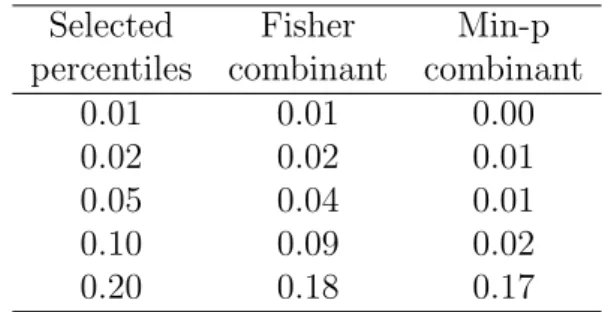
The number of sampling R is equal to 120. Two combination functions are used: the Fisher (green dashed) and the min-p (black dotted). The blue line is the uniform CDF. On the right-hand side, the table of some selected percentiles of the p-values presented graphically in the adjacent figure. . . 25 2.4 On the left side are displayed the kernel density estimates of four

kine-matic variables for background (red) and signal (blue). On the right panel a mixture of 90% background and 10% signal (blue) is compared to the background alone (red). A Gaussian kernel and Silverman’s “rule of thumb” for bandwidth selection are used (Silverman, 1986, p.48). . . . 31 2.5 On the left hand side, it is shown the kernel density estimate of marginal

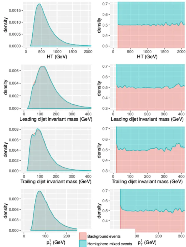
distributions for the chosen kinematic variables (Section 2.4.1) of pure background (red) and their respective hemisphere mixed background data (blue). On the right hand side, the normalised stacked plots of the kernel density estimates. . . 32

(18)

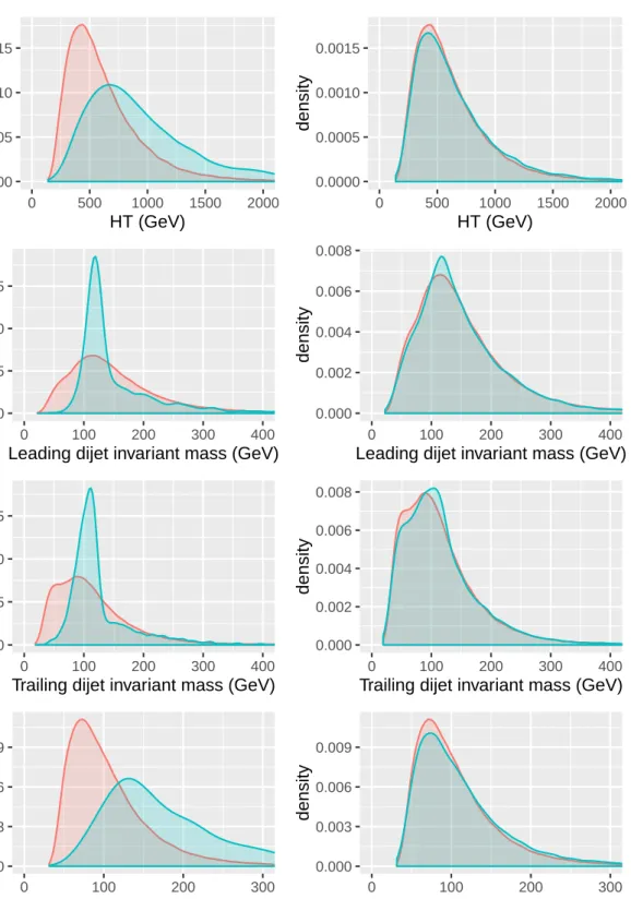
2.6 Left: comparison of the distributions of the four kinematical variables for background alone and the hemisphere mixed data of a sample constituted by 10% signal and 90% background. Right: stacked plots of the estimated densities. . . 33 3.1 Example of informative and uninformative variables for density

estima-tion. The first one has a more complex density (in blue) and is modelled by the two separated mixture components (in black), while the second one has component means shrunk to 0 and hence is modelled by a single Gaussian. . . 42 3.2 Performance comparison for the 5 model-based clustering methods given

the datasets of sizen= 250 andn= 500 generated from the two Gaussian components for the varying separation (mult). . . 52 3.3 Performance comparison for the two types of variable selection

meth-ods (M1 and M2) for the MESP and the datasets of size n = 250 and

n = 500 with varying separation (mult). The results are based on an average model performance on 50 simulated datasets generated from the two Gaussian components. . . 53 3.4 Performance comparison for the 5 model-based clustering methods given

the datasets of size n = 250 and n = 500 generated from the three Gaussian components for the varying separation. . . 54 3.5 Performance comparison for the two types of variable selection methods

(M1 and M2) for the MESP and the datasets of sizen= 250 andn = 500 with varying separation (mult). The results are based on an average model performance on 50 simulated datasets generated from the three Gaussian components. . . 54 4.1 The Inverse Bagging scores computed based on the test statistics for the

varying sample size Q plotted against the simulated univariate data. In legend the respective AUC values are shown. . . 70 4.2 The ROCs and their corresponding AUC values in the legend for the

Inverse Bagging scores computed based on the Ok scores computation method for the varying sample size Q and a number of the performed sampling (expressed by the parameterE(T riedl)) for one of the simulated

datasets. . . 71 4.3 The AUC performance of the Inverse Bagging for the different parameter

Q and the simulated multivariate datasets. In blue it is denoted the mean Inverse Bagging performance which in its maximum reaches the performance of the mean LDA score (in red). . . 72 4.4 The AUC performance of the Inverse Bagging for the varying parameter

Q and the simulated datasets with a spherically distributed signal. In blue it is denoted the mean Inverse Bagging performance and in red the average performance of the LDA score. . . 72 4.5 The AUC performance of the Inverse Bagging for the different

parame-ter Q and the simulated datasets with signal uniformly distributed on a hemisphere. In blue it is denoted the mean Inverse Bagging performance and in red the one of the LDA score. . . 73

(19)

List of Tables

2.1 Test statistics for performed tests on the B + 1 permuted datasets re-garding the S subsets of variables. . . 22 2.2 Overview of p-values computation given the corresponding test statistic

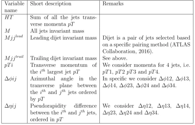
values from Table 2.1. . . 22 2.3 Description of the 20 considered data variables for the multijet final state

analysis. . . 24 2.4 Fraction of cases for which the null hypothesis was correctly rejected by

the KDE permutation test with the Fisher combinant for significance levels α equal to 0.01, 0.05 and 0.10. 80 pairs of samples were generated under the alternative hypothesis for each background contaminated data with values of signal fraction s equal, in turn, to 1%,5% and 10%. . . . 27 2.5 Obtained p-values for the KDE tests in the permutation framework to

verify if the Hemisphere Mixing approach performs according to its pur-pose. The tests are performed on samples of size n = 15000. . . 30 3.1 Anomaly detection results for the different data generating scenarios and

the M1 and M2 dimensionality reduction approaches compared with the fixed background model (FBM). Given 50 simulations for each scenario, the average ARI and AUC measurements are computed based on the training datasets and the AUC based on the independent testing set. . . 56 3.2 Description of variables used for the application to anomaly detection in

context of the high energy physics. The detailed definition of the used variables can be found in (Chen, 2012). . . 57 3.3 Summary of the anomaly detection results performed by the PAD M2

and the fixed background model (FBM) for datasets with different signal proportions λ. For each scenario, 50 datasets are generated to obtain a mean result with the respective standard deviations presented in brackets. 58 4.1 The mean performance of the Inverse Bagging regarding the AUC for

the different methods of scores computations and diverse sample size Q

shows a superior performance for the method based on the test statistics. The mean AUC for the LDA score is 0.760. . . 70 4.2 The mean performance of the Inverse Bagging regarding the AUC for

the different methods of scores computations and varying samples sizeQ.

The mean AUC of the LDA score is 0.904. . . 71 4.3 Results of the Inverse Bagging using specific quantiles of test statistics

for the scores computation. The 4 different quantiles are considered and compared with the averaging method. . . 77

(20)

4.4 Mean performance of the different variable sampling approaches regarding the AUC. The parameter L controls the number of selected variables for testing. The mean AUC of the LDA scores is equal to 0.865 and of the standard Inverse Bagging with Q= 50 is 0.862. . . 78 4.5 Mean AUC of the weighted sampling approaches for the varying

param-eter L given different combinations of using weights withing sampling approaches denoted by T -True - and F - False. The mean AUC of the LDA scores for the generated datasets is equal to 0.865. . . 78 4.6 Mean AUC of the Inverse Bagging approaches on the correlated data for

the varying parameter L. The mean AUC of the LDA scores is 0.907. . . 79 4.7 The Inverse Bagging classification performance using the AUC for the

4% mixed data with and without the prior Cholesky data transformation (column ”Rotation”). The AUC for the LDA score is 0.839 and the one of the standard Inverse Bagging is 0.851. . . 81 4.8 Performance of the Inverse Bagging regarding the AUC on the physical

data for several considered anomaly detection approaches; from left-hand side for the standard Inverse Bagging, the improved version of the Inverse Bagging – the max-10-sampling with the parameter L_{∈ {}5,8_}, the LDA score and the PAD from Chapter 3. Results are obtained for varying signal proportion λ based on 50 generated datasets. . . 82

(21)

(22)

(23)

Introduction

Overview

Since the early Seventies, the Standard Model has represented the state of the art in Particle Physics. It describes the structure of the Universe - the elementary particles, and the inherent interactions - the fundamental forces. Despite its apparent empirical confirmations, it is evident that the Standard Model is not a complete theory, as it fails to explain several phenomena like, for instance, the gravity, the nature of dark matter, and the dark energy. For this reason, there are persistent attempts to either extend the Standard Model or to build an entirely new theory (Grossman and Rakshit, 2004). To this aim, physical experiments are conducted within large accelerators, as e.g., the LHC at CERN. The experiments involve propelling charged particles, making them collide and detecting the created products. Collected data are then used to validate and delve into physical theories or to find evidence of possible new physics, not predicted by the Standard Model.

In broad terms, two physical processes are of interest within the considered frame-work: the background process refers to the known physics described by the Standard Model. Although well rooted by definition, and with the due specifications which will be clarified in the rest of the thesis, the knowledge of such process is required to be deepened for specific purposes. The latter process, referred to as signal, represents, in turn, the unknown physics, which is required to complete our knowledge of the Universe. While the physical theory allows for conjecturing possible expressions for such process, its existence is itself brought into question and, whenever acknowledged, it is required to expect its extreme rarity.

In this framework, statistics plays a pivotal role, aiming at providing tools to analyse the data and thus answer the physical research questions. In this perspective, and consistently with the aforementioned problems, this thesis addresses the following goals: 1. Improving the accuracy in estimating the probability density function underlying

the background process.

(24)

2 Main contributions of the thesis

2. Providing the tools to identify a possible, unknown, signal and to discriminate it from the background process.

Main contributions of the thesis

Stemming from a characterization of the aforementioned research goals, in the fol-lowing, the investigation path which has been pursued to attain them, as well as the main results of the thesis are summarised.

• Despite that the background process represents, by definition, the known physics, its probabilistic generating mechanism is not explicitly defined or numerically computable, and requires to be estimated. However, the background data needed to estimate the underlying probability density function are not always accurate or available. To circumvent the problem, Dall’Osso et al. (2017) have designed an algorithm aimed at generating background-like data. A statistical validation is then necessary to test whether the method performs according to its goals. The problem can been framed in a hypothesis testing framework, with the null hy-pothesis establishing the equality of two distributions. While this problem admits, in principle, a number of standard solutions, the available approaches are based on specific assumptions that do not hold in the considered application, where data at hand are multivariate and exhibit non-Gaussian properties, such as skewness and multimodality.

Duong and Schauer (2012) have proposed a kernel density-based global two-sample test, which appears suitable for the application. However, nonparametric methods are particularly affected by the curse of dimensionality which prohibits their use for high dimensional data.

As a first contribution of the thesis, it is proposed to perform the mentioned test multiple times in low-dimensional subspaces, and apply a proper combination function to the obtained results for verifying the previously stated hypothesis. Due to correlations between the multiple test results, statistical inference from their combination is not straightforward. For this reason, it is proposed to embed the test in a permutation framework, which allows for obtaining the empirical distribution of the combination function values under the null hypothesis. The obtained permutation-based two-sample test is validated concerning its first type error rate and its power. Finally, it is applied to the physical data to answer the primary question of interest.

(25)

Introduction 3

• The main assumption underlying empirical searches of new physics is that any possible signal would behave as a deviation from the background process. From a statistical perspective, the problem can be then expressed in the framework of anomaly detection, where observations not consistent with the assumed back-ground model are searched in the experimental data (Pimentelet al., 2014). Unlike above, in this setting the background process is entirely known and a sample of virtually infinite size can be drawn from it. Two different sources of data are then available: a first sample generated from the background process - in the following referred to as labelled since the generating process of the observations is known, and a second, unlabelled experimental sample, whose generating mechanism is unknown, as it surely include observations from the background but might also include observations from the signal. The anomaly detection problem can be then faced according to a semi-supervised approach, due to the partial labelling of the available data.

Among several alternatives, in the thesis two different approaches to the semi-supervised anomaly detection problem are followed:

– The first approach stems from the idea of semi-supervising the signal de-tection by strengthening unsupervised (clustering) methods via the inclusion of the additional information available on the background. The proposed method originates from the family of model-based clustering approaches, and assume Gaussian mixtures densities to model the background and sig-nal distributions. Due to the curse of dimensiosig-nality, the approach can be sub-optimal or even not feasible to be performed on high-dimensional data. Pan and Shen (2007)) and Xie et al. (2008) introduce penalised methods for variable selection in the context of model-based clustering, but rely on restrictive assumptions on the covariance matrices of the clusters. In the the-sis, the penalised approach is extended to allow for a more flexible modelling without constraining the mixture component covariance matrices. Addition-ally, a variant of the Expectation-Maximization algorithm (Dempster et al., 1977) is derived and implemented, to estimate the parameters of the mixture model via the numerical maximization of the penalized likelihood function. Subsequently, the idea of variable selection within model-based clustering is extended for anomaly detection purposes in the semi-supervised setting, starting from the works of Vatanen et al. (2012) and Kuusela et al. (2012). – The second approach for semi-supervised anomaly detection phrases the

(26)

4 Main contributions of the thesis

experimental data if there is evidence that such data are not compatible with the background probability distribution. This natural idea has been developed by Vischia and Dorigo (2017) which make use of sampling and multiple hypothesis testing to study anomalous properties of data at hand. The proposed procedure depends on many parameters, but their influence on the method performance has been yet unclear. In the thesis, an optimal selection of such parameters is studied both theoretically and based on sim-ulations. The performance of the procedure is validated and compared with competing methods given artificial data and within applications to real ones. Some improvements of the method are proposed concerning its performance for high dimensional data.

The rest of the thesis is organized as follows. In Chapter 1 an overview of the phys-ical framework is provided. Chapter 2 introduces the problem of background density estimation, illustrates the physical procedure for generating background data, discusses and validates the proposed permutation test. Chapter 3 and 4 focus on the signal de-tection problem, and illustrate the clustering-based and, respectively, the hypothesis testing-based procedures.

(27)

Chapter 1 The physical framework

1.1 The Standard Model

Since the dawn of time, men have been trying to make sense to the surrounding word. Over the years, incredible progresses have been done in understanding the physics of the Universe, ranging from the microscopic scale of atom building quarks, to giant stars and quasars. One question of interest concerns understanding the structure of the Universe - the elementary particles - and the inherent interactions -the forces. Physical theories provide an effective mathematical formulation describing physical systems, subsequently validated and possibly confirmed based on physical experiments specifically designed. Once a theory is confirmed it becomes a starting point for further extensions which, in turn, allow for a more accurate description of the world.

Over time, particle discoveries, as for example, the ones of electron (1896), proton (1919) or neutron (1932), have allowed for a rough understanding of matter building blocs. With the increasing knowledge of the universe structure, an advance in under-standing the physical forces has been made. Four fundamental particle interactions have been classified - namely the electromagnetic, weak interaction, strong interaction and the gravitational forces. Around 1970 a complex theoretical framework was established to comprehensively describe the elementary particles known at that time, and three of the four fundamental forces (gravity not included). The theory, referred to as the Stan-dard Model, postulates the existence of matter constituents - the fermions (see Figure 1.1) - and the mediators of interactions - the bosons (see Figure 1.2). Fermions and bosons are characterised by the electrical charge, spin and a life-span, which establish their properties, possible interactions or bounding configurations.

At the time of the first Standard Model formulation, many of the model-assumed elementary particles were not empirically discovered yet. Only recently the last missing

(28)

6 Section 1.1 -The Standard Model

Figure 1.1: The twelve postulated fundamental constituents of matter in the

Stan-dard Model - fermions (Thomson, 2013).

Figure 1.2: The four known forces of nature. The relative strengths are

approxi-mate indicative values for two fundamental particles at a distance of 1f m= 10−15_m

(Thomson, 2013).

elements of the Standard Model have been proved - the top quark (CDF Collaboration, 1995), the tau neutrino (DONUT Collaboration, 2001) and the Higgs boson (ATLAS Collaboration, 2012; CMS Collaboration, 2012). The modern discoveries deeply rooted the Standard Model (with some later adaptations) to be the current widely-acceptable state of the art of the physical theory.

Although the Standard Model is sometimes claimed to be a uniform theory of ev-erything, the physical community is far to consent with such statement. The Standard Model is not a self-contained theory, as for example, it does not account for the gravi-tational force; it is not able to explain the mechanism of the dark matter creation, the neutrinos non-zero mass and many other phenomena (Fuks, 2012). For these reasons, there are persistent attempts to either complete the Standard Model or to build an en-tirely new theory (Grossman and Rakshit, 2004). In general, any further development of the current state of art needs to address the two following questions of interest:

1. Is it possible to improve our knowledge within the Standard Model framework? 2. Is it possible to go beyond the Standard Model, by completing it or defining an

alternative theory?

With some due specifications, these are the general problems on which the thesis focuses. The aim is pursued via an investigation of suitable statistical methods aimed

(29)

Chapter 1 - Background and motivation 7 at providing an answer to these questions.

1.2 The experimental settings

A natural way to answer the central research questions is to design and perform suit-able experiments to find a required justification. Nowadays, such physical experiments and the experimental infrastructures to make them possible are incredibly complex, costly and require years of careful planning before any answer could be found. The complicated process of an experiment design is only sketched underneath, as our fo-cus is instead put on statistical analyses of collected experimental data to find possible evidence for backing up any theoretical claims.

In general, experiments with elementary particle physics often require the use of very high energy to allow for an insight into processes that are rare or do not occur at low energy. For this aim, specific infrastructures are built - namely particle acceler-ators, that use an electromagnetic field to propel charged particles to nearly the light speed. There are many accelerators types with different topological structure (linear, circular) or mechanical design (electrostatic, electrodynamic) but have the common aim of increasing particle kinematic energy to a given high value. The currently most fa-mous accelerators from their impact on discoveries are the LHC (CERN, Switzerland),

Tevatron (Fermilab, the USA) and KEKB (KEK, Japan).

For the high energy physic purposes, recent accelerators are often built in a circular shape - the so called synchrotrons. Such design allows for a continuous acceleration of groups of charged particle - beams - to reach an exceptional energy of the propelled particles. The LHC is a record holder for reaching the energy equal to 6.5T eV, in which particles are accelerated in an underground ring of circumference equal to 27 km. Usually, in synchrotrons, two beams are accelerated in opposite directions and cross in specific locations where the propelled particles collide.

Each particle collision, referred to as an event, produces complex individual inter-actions, i.e. state transitions, hadronisation, bosons and quarks production, particles decay, and others. Large particle detector systems are placed around the collision points, to enable reconstruction of the primary particles produced for each event. Such detec-tors are highly-advanced sensors which use a wide range of technologies to identify and measure properties of the produced particles. In general, detectors are cylindrically shaped barrels stretched along the beam path. They consist of specific zones for particle tracking (an inner region) and calorimeters for their energy measurements. See Figure

(30)

8 Section 1.2 - The experimental settings

Figure 1.3: Typical layout of a particle detector equipped with a tracking system

(here shown with cylindrical layers of a silicon detector), an electromagnetic calorime-ter (ECAL), a hadron calorimecalorime-ter (HCAL) and muon detectors. Usually, around the detector a solenoid is wrapped (not shown in Figure) to produce the magnetic field which bends the charged particles trajectories (Thomson, 2013).

1.3 for a schematic detector cross-section. Outside of the colourimeters, additional lay-ers of muon detectors are often placed. Ideally, all the produced particles (apart from neutrinos) should be absorbed by the respective sensors and their existence evidenced. In the LHC at CERN, there are two main particle detectors: ATLAS, which has around 25 meters of diameter, and the more compacted CMS detector.

For each high-energy collision event, many particles can be produced. For each particle, its energy and a 3-dimensional momentum are measured, respectively by the calorimeters and the tracking elements of the particle detector. The four variables - the so called 4-vector - are necessary to identify each collision product distinctly. In the LHC a Cartesian coordinate system is defined as follows: the origin is located at the collision point, the x-axis points to the centre of the ring, the y-axis vertically upwards and the z-axis is tangent to the beam. Alternatively, an equivalent system of polar coordinates is used which is invariant under certain transformations. The azimuthal angle φ is measured in the xy plane from the x-axis and the radial coordinate in the plane is denoted by r. The polar angle θ is defined in the rz plane but preferably it is expressed in terms of the pseudorapidity η = ln tan θ₂

. The transverse momentum - pT - is computed as the momentum component perpendicular to the beam direction. Similarly, the transverse energy is defined as ET =Esinθ where E is the total energy.

Due to a very high frequency of collisions, the amount of the possibly produced data is so large that only a small percentage can be filed. Specifically designed hardware and software solutions, the so called triggers, allow for filtering out only observations

(31)

Chapter 1 - Background and motivation 9 of potential interest, i.e. the part of the data to be discarded is redundant as it is associated with already well-known processes (CMS Collaboration, 2016b). Later, for events admitted by the triggers, a particle identification needs to be accomplished by specific software solutions based on the recorded tracks, energy deposits and the known physical theory (CMS Collaboration, 2009). Unfortunately, the identification is not straightforward as some particles quickly decay before they reach calorimeters. An example is an energetic quark which decays by radiating gluons along its way so that its initial energy cannot be directly measured. However, the quark generates bunch of gluons which travel in approximately the same direction so that a cone is formed - a phenomenon referred to as the jet formation. Jet measurements allow for later reconstruction of energy and momenta for the decayed quark. The summary of all the identified particles of a given event (for example one electron and two jets identified for an event) are referred as the event final state. After all these steps, the preprocessed experimental data are finally prepared for the analysis purpose. In conclusion, the data consist of automatically selected events where each of them is composed of a list of identified particles with their respective measurements - the 4-vector.

1.3 Motivation

1.3.1 Improvement of the knowledge within the Standard Model

framework

The Standard Model framework describes possible outputs and interactions of phys-ical phenomena in probabilistic terms but, in general, a probability distribution of col-lision kinematic or angular variables is unknown. In principle, such distribution could be computed by solving multivariate integrals of partition functions and nonlinear La-grangians. However, for computational and numerical reasons this is not feasible to be performed. Hence, the probability distribution of the physical process described by the Standard Model, in the following referred to as the background, is required to be esti-mated. In fact, the problem is not trivial, due to the lack of reliable background data. Experimental data are not directly usable, as they are realizations of some, more compre-hensive, possibly unknown process, whose the background represents only a (dominant) fraction.

Conversely, background estimation is often based on Monte Carlo simulations, per-formed under the assumption that the Standard Model is correct. Unlike statistical simulations, aimed at generating data given their distribution, physical Monte Carlo

(32)

10 Section 1.3 -Motivation

simulations are based on a different concept, i.e. a probability density function of vari-ables is not necessary to produce a related sample. Such simulated data consist of realisations of possible collisions which are produced by a complex system of adequate generation steps. Without going into the physical details, based on theoretical parton distribution functions, possible collision effects are simulated in an appropriate propor-tion and with respect to the physical rules, i.e. via the creapropor-tion of elementary particles, coupling, their interactions and others. The simulations also cover other processes that the produced particles undergo immediately after the collision, as for example their de-celeration, scatterings or jet creation. For such simulated events, a detector response is computed based on its measurement efficiency. Later, a specific trigger is applied, to reflect circumstances in which the experimental data are collected. Finally, a parti-cle identification is performed leading to the collision reconstruction. To facilitate the complex computation, many specific software packages have been implemented for this aim, as for example “MadGraph” (Alwallet al., 2014), “Pythia” (Sj˝ostrandet al., 2006, 2015), or “Delphes” (de Favereau et al., 2014).

Hence, simulating data from the background process is possible, and frequently per-formed, so that for many final states of particle collisions the generated data are tolerably accurate. Nevertheless, given the degree of complication, some simplifications need to be applied for facilitating the simulation procedure. For example, to avoid computations of multivariate integrals describing complex particle states, approximation methods are used (Frixione and Webber, 2002). Also, not every physical phenomenon is predictable, for instance, whenever the strong force plays a relevant role. In all these circumstances, simulations get imprecise or biased. Additionally, for some rare processes, it can be impossible to produce large data quantity as they are computationally too expensive to be generated.

To respond to the scarcity or the inadequacy deficiencies of Monte Carlo data for complex final states, Dall’Osso et al. (2017) have designed a novel approach that ad-dresses the issue of generating background-like data, referred to as the Hemisphere Mixing. They propose to use the experimental data themselves which might include non-background observations, and apply a specific permutation scheme, referred to as a mixing procedure. The mixing is driven jointly by the knowledge of the physical process and information from the experimental data. It aims at transforming all the input data into observations distributed according to the dominant background process - to be used for estimating the background density.

In experimental particle physics, the mixing approach is not novel, but uncommon. The method has turned out to be successful for some specific applications, as for example

(33)

Chapter 1 - Background and motivation 11 electron-positron collisions (CMS Collaboration, 2010, 2011b). However, for complex final states of the proton-proton collisions occurring at the LHC, the idea has never been used. In specific, Dall’Osso et al. (2017) have adjusted the mixing definition to make it suitable for the multijet collisions.

Although there is a physical and logical reasoning behind the Hemisphere Mixing approach, it needs to be formally verified if the method performs appropriately to its goals. These are:

1. From input data generated dominantly by the background, the Hemisphere Mixing produces data entirely distributed according to the background.

2. Distributions of input data and the related hemisphere mixed output data are equal, if and only if the input data are the background.

The aforementioned questions are addressed in Chapter 2, via an introduction of a suitable statistical test.

1.3.2 Going beyond the Standard Model

Another fundamental research direction within the physical community follows the need of developing the current theory. This can be achieved either by extending the Standard Model or by constructing an entirely new physical framework (Fuks, 2012). Research is often performed based on a data-driven evidence of new physics which can appear, for instance, as a sign of a new particle unpredicted by the Standard Model.

There have been several efforts in new physics searches within the community. Such searches are often driven in a model-dependent guise where supervised classifiers are trained to find particular phenomena expected to be seen under hypothetical theory ex-tensions (ATLAS Collaboration, 2014b; CMS Collaboration, 2016a). As a result, only a narrow subspace of possible alternative extensions is tested. Without being constrained to any physical hypothesis, a more general approach - called model-independent - has also been applied in this context (CMS Collaboration, 2011a, 2017; ATLAS Collabora-tion, 2014a, 2017; Popov, 2011). Such approach allows the data to speak for themselves and searches within a broader range of alternative signal processes. It aims at new signal detection rather than confirmation of any physical theory.

The main assumption underlying model-independent searches is that new possible physics - referred to as a signal process - would show an anomalous behaviour with respect to the background. In the considered setting, Monte Carlo simulations are usually trusted to provide accurate data from the background and feasibly produced

(34)

12 Section 1.3 -Motivation

with an arbitrary size. Hence, the problem of detecting a possible signal can be ad-dressed according to a semi-supervised approach, by comparing the the Monte Carlo data generated from the background, with the experimental ones, which might include observations from the signal.

This problem is addressed in Chapters 3 and 4, by considering two alternative logics, based on the semi-supervision of clustering methods and the employment of hypothesis testing respectively.

(35)

Chapter 2 Validation of a physical algorithm

to improve background estimation

2.1 Motivation and goals

The background process is defined by the Standard Model established on the known physical theory, however, its underlying probability density function is generally un-known and requires a precise estimation. Such goal has been usually attained relying on Monte Carlo simulated data. Nevertheless, simulations are suitable only for some scenarios for which the artificially generated data can be trusted and are available in large quantity. Otherwise, the density estimate is unobtainable or inaccurate. The issue of the Monte Carlo data imperfectness is present for instance in multi-jet final states analysis, which is especially useful for a more in-depth understanding of the Standard Model. In specific, non-resonant pair production of Higgs bosons decaying into a b¯bb¯b -quark final state provides an excellent measure to determine the self-coupling λ - a crucial Standard Model parameter. However, as the multi-jet final states have a high potential for a more exhaustive understanding of the Standard Model, it calls for inves-tigating of novel methods that can replace the insufficient Monte Carlo simulations and improve the required background estimation.

An ideal solution to overpass the aforementioned issue would be to generate back-ground data completely (or at worst approximately) independent on the underlying physical theory. Within this logic, the Hemisphere Mixing algorithm has been recently proposed by Dall’Ossoet al.(2017). It takes as an input the experimental collision data

Y,and applies on them a specific permutation transformation driven by the knowledge of the physical context so that new synthetic data _Z are produced. Under the assumption that the input data are generated entirely (or at least dominantly) by the background

(36)

14 Section 2.2 - Description of the Hemisphere Mixing algorithm

process, it is aimed that the generated data _Z have the background distribution. Pro-vided that the method works according to its goal, it could be successively used for the production of background samples from the experimental data _Y without resourcing to either Monte Carlo simulations or being heavily based on the physical theory.

From the statistical point of view, an extended analysis needs to be performed to verify if the Hemisphere Mixing algorithm produces data with adequate properties, i.e. distributed according to the background density. Ideally, a two-sample statistical com-parison test should be applied to the background data and the hemisphere mixed output data to verify if the algorithm application can retain the data background properties and smear out the signal evidence if present. A permutation-based hypothesis test is introduced for this aim, its type-1 error and power are evaluated. The test is applied to physical data in several scenarios so that the algorithm performances for specific conditions are verified.

2.2 Description of the Hemisphere Mixing algorithm

The Hemisphere Mixing algorithm is based on the so-called observation mixing ap-proach. In a shorthand, each input event is adequately replaced with components orig-inating from other events. For each event, the algorithm groups collision jets into two disjoint sets and reconstitutes them using different sets with similar properties. The selected sets are jointed so that a new event is composed, and if applied to all the events, the algorithm output is produced. The mixing idea per se is not utterly new in physical applications (CMS Collaboration, 2010, 2011b) but it had required in-depth adjustments for the peculiar application setting, and to our knowledge, it has never been applied to the multi-jet studies.

Let us consider proton-proton collisions resulting in the production of multiple jets originating from collision points. As it has been explained in Section 1.2, each particle and jet can be distinctly defined by specifying their measured 4-vectors. However, to compare events, it is required to use more general event summary statistics as collisions can differ in the number of produced jets, and, in principle, the jets are not ordered. In practice, various event-based statistics are computed from the corresponding 4-vectors which give rise to data variables. The variables are chosen so that they have a meaningful physical interpretation, they are invariant under certain transformations or powerful for the background and a possible signal discrimination.

The first step of the algorithm is to bi-partition the event jets so that the two resulting sets have possibly null or negligibly small between-group physical interactions. This is

(37)

Chapter 2 - Background estimation 15 performed within the data framework defined in Section 1.2 using a “thrust” axisTTT .The axisTTT is determined in the Euclidean coordinate system separately for each event based on its jet momenta. It passes through the collision point and its direction is specified in the way that event jet momenta projections along it are maximised, i.e.

argmax N j X h=1 ||ppph|| |cos ∆ (ppph, TTT)| ! , (2.1)

where N j is a number of the event jets, ∆ (ppph, TTT) is the angle between the hth jet momentum vectorppp and the thrust axisTTT .

A perpendicular plane to the thrust axisTTT ,which passes through the collision point, divides the event topological space into two sub-spaces. Each subspace and jets enclosed in it are referred to as the hemisphere. A graphical visualisation of a collision, its resulting jets, the respective thrust vector and the hemisphere division is presented on the left-hand side of Figure 2.2.

A fundamental assumption of the Hemisphere Mixing algorithm is that interactions between event hemispheres are negligible. The independence assumption should be ex-plained based on the known physical principles at least to the so-called “first order” effects. In fact, for the considered proton-proton collisions at the LHC, the produced hemispheres are dependent as, in general, the event centre of mass is not at rest. How-ever, if the phase space is reduced to the transverse plane in which the thrust axis is bounded to be determined, the independence assumption holds, and the hemispheres are only related by the QCD radiations, pile-up effects or multiple parton scatterings (the detailed explanation is given in AMVA4NewPhysics ITN, 2017). Thus, without loss of generality, we consider only a 2-dimensional space of the transverse plane in which the thrust axis is determined.

The experimental data_Y of sizem are supplied to be the Hemisphere Mixing algo-rithm input. Forl = 1, ..., m,the algorithm takes subsequent observations for which the respective thrust axis are determined and two corresponding hemispheres are obtained. Note that the hemispheres are ordering invariant, and, without loss of generality, let us denote them ash2l−1 and h2l. After all the iterations, a total of 2m hemispheres are

col-lected to compose the so-called hemisphere library. In general, using the independence assumption of the hemispheres, one could pick at random two hemispheres from the library, merge them up and obtain a possible valid event of the multi-jet proton-proton collision. The following variables describe the hemispheres: the number of jets they in-clude N j, the number of b-tagged jets N t (a specific type of jets), the sum of projected jets transverse momenta along the thrust axis T, the combined mass of jets M, the sum

(38)

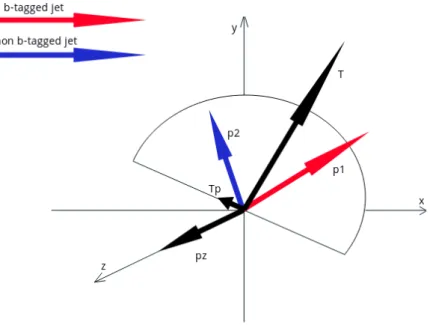
16 Section 2.2 - Description of the Hemisphere Mixing algorithm

Figure 2.1: Graphical representation of an example hemisphere containing two jest

(N j= 2) with respective massesm1 andm2 and transverse momentap1 andp2. One

jet is b-tagged N t = 1; the combined mass M = m1+m2; T and T p are chosen

according to Equation 2.1.

of momenta projections perpendicular to the thrust T p, and the sum of jets momenta components along the z-axis P z.An example graphical representation of a hemisphere is presented in Figure 2.1. From one perspective each hemisphere can be seen as a point in a 6-dimensional space with the associated variables N j, N t, T, M, T p and P z.

After construction of the hemisphere library, the mixing procedure can be performed. Forj = 1, ...,2m, an iterative search within the Hemisphere library is performed to find the most similar hemisphere to the current one hj. The similarity between the jth and kth hemispheres, for k _{∈ {}1, ...,2m_{} \ {}j_}, is defined by a distance measure D(l, k) expressed in the hemisphere feature space as

D

(

j, k

)

2

=

(T(hj)−T(hk)) 2 V ar(T)

+

(M(hj)−M(hk))2 V ar(M)

+

(T p(hj)−T p(hk))2 V ar(T p)

+

(|P z(hj)|−|P z(hk)|) 2 V ar(P z)

,

namely the Euclidean distance scaled by the variable variances. Additionally, if the hemisphereshj andhk differ for any valuesN j orN t the distance is set to +∞.Finally,

a hemisphere hk with the smallest distanceD(j, k) tohj is selected as the most similar. Let us denoted such hemisphere hk by hlibj as the closest to hj from all the ones in

the library. Such search can be performed using a kind of a multi-dimensional nearest-neighbor approach (Bentley, 1975). New events – the algorithm output – are constructed

(39)

Chapter 2 - Background estimation 17

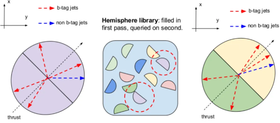
Figure 2.2: Graphical visualization of an original collision event (the left-hand side)

and a corresponding created artificial event (on the right-hand side) from two closest hemispheres selected from the hemisphere library (central diagram). Figure originates form AMVA4NewPhysics ITN (2017).

Algorithm 1 Pseudo-code of the Hemisphere Mixing Input: experimental data _Y

Parameters: distance measure function D(j, k) 1: m _← size of the data _Y

2: allocate HemLibrary - an empty set 3: for l= 1, ..., mdo

4: determine a thrust axis for the observationyyyl

5: bi-partitionyyyl and produce hemispheres h2l−1 and h2l

6: store h2l−1 and h2l in HemLibrary

7: end for

8: compute a distance matrix based on the functionD(j, k) between all the hemispheres from HemLibrary

9: for j = 1, ...,2m do 10: hlib

j ← the closest hemisphere from hj within the HemLibrary (excluding hj)

11: end for

12: for l= 1, ..., mdo

13: zzzl ← merged hemispheres hlib2l−1 and hlib2l

14: rotate zl according the the lth thrust axis to closely correspond toyyyl

15: end for

16: return Data _Z consisting of eventszzzl for l= 1, ..., m.

from the selected hemispheres, specifically, for l = 1, .., m, the two found hemispheres

hlib

2l−1 andhlib2l corresponding to thelthobservation are merged up. Each constituted new

artificial event is also appropriately rotated so that it matches the thrust axis and closely corresponds to the original one. Figure 2.2 gives a graphical overview of the presented idea and for a exhaustive explanation of the Hemisphere Mixing see Algorithm 1.

(40)

18 Section 2.3 -Statistical question of interest

The outlined Hemisphere Mixing algorithm produces entirely new data_Z,referred to as thehemisphere mixed data. The mixing is designed to possibly preserve the dominant properties of the input data, for example, the marginal distribution of their kinematic variables. Hence, it is expected that the hemisphere mixed data produced from the background sample keep their inherent background distribution.

On the other hand, if the experimental input data include observations from the sig-nal process, then the mixing procedure is expected to smear out the sigsig-nal features, i.e. purify the mixture data to produce fully background-like distributed observations. It is presumed that due to the small number of signal observations, the hemisphere library is going to be poorly represented by the signal-originated hemispheres; consequently, it is likely to model the signal observations using the background originating hemispheres. Such modelling is expected to yield the dominant process properties. However, if the hemisphere similarities are determined by variables greatly discriminating the back-ground and signal processes, then the signal events are likely to be reproduced using the signal originating hemispheres, and the expected smearing does not occur. In any case, whether the signal is present, some background observations can be wrongly modelled using at least partially the signal originating hemispheres, which can severely degrade the algorithm performance.

2.3 Statistical question of interest

2.3.1 Description of the problem

Let us introduce a notation for the datasets at hand. Denote the experimental data _Y = (yyy1, ..., yyym)0, where yyyl = (yl1, ..., ylp, ..., ylP)0, l = 1, ..., m, are supposed to

be i.i.d. realizations from an unknown probability density function fBS : RP → R.

Consider also a background density fB : RP → R which refers to the known processes

predicted by the Standard Model. If the process generating the experimental data _Y does not contain any signal component then naturally the distributions fB and fBS are equal. The hemisphere mixed data _Z = (zzz1, ..., zzzm)0, where zzzl = (zl1, ..., zlp, ..., zlP)0, l = 1, ..., m, are realizations from an unknown probability density functionfOut :RP → R. Note that all the mentioned densities (fBS, fB and fOut) are in practice unknown.

For the general case for which the algorithm is designed, the background data are not available due to the described issue of the Monte Carlo simulations. However, for the algorithm verification purpose, such collision scenario is chosen that the background and signal data are feasible to be produced in a large quantity. In specific, two datasets are generated: the background data _X = (xxx1, ..., xxxn)0, where xxxi = (xi1, ..., xip, ..., xiP)0,

(41)

Chapter 2 - Background estimation 19

i = 1, ..., n i.i.d. realizations from the background density fB and the respective signal

data from the density fS which are used to generate the experimental data Y.

In order to verify the performance of the Hemisphere Mixing algorithm, a formal statistical test has to be applied, to provide evidence that the density fOut of the

hemi-sphere mixed data _Z is equivalent to the background one fB, whether the input data Y

include signal or not. The null hypothesis is

H0 : fB(·) = fOut(·)

against the alternative

H1 : fB(·)6=fOut(·).

The issue of testing two samples for a common distribution is quite common for statistical application. The literature well describes many potential solutions (Tinsley and Brown, 2000). The most well-known is the Kolmogorov-Smirnov test (Sheskin, 2003) whose test statistic is computed based on a distance between empirical cumula-tive distribution functions of the two compared samples. The test can be used only for unidimensional data, but it has several other attractive features; among them it is the robustness to outliers, as the statistic is just sensitive to the bulk of density function. On the other hand, the test usually has small power in comparison to others (Razali

et al., 2011). Multivariate extensions of the Kolmogorov-Smirnov test have been pro-posed. However, they are computationally complex and do not scale well with the data dimensionality (Friedman and Rafsky, 1979; Justel et al., 1997).

A more powerful substitute is the Wilcoxon rank sum test (Sheskin, 2003). This is a common nonparametric univariate two-sample test, for which the alternative hypothesis is that the two distributions differ by some location shift µ₆= 0 (for the two-sided case). For the considered data this test is not suitable as it is not multivariate and tests a different hypothesis (the same location, in general, does not mean the equality of distributions).

Next, the Multivariate Analysis of Variance (MANOVA) (Sheskin, 2003) seems to be a better alternative as it is oriented at multidimensional cases. However, the test is designed to spot the difference in means, and therefore it also does not satisfy the meant hypothesis. Additionally, the assumption for the test is that the variables have Gaussian marginal distributions which is not the case for the data at hand (Figure 2.5). However, for a large number of observations the distribution of the sample mean is approximately normal (as it follows from the Central Limit Theorem) and for this reason, its use to some extent can be judged (Khan and Rayner, 2003).

(42)

As described above, these standard statistical tests are not proper for our purpose. For this reason, we have to identify a more sophisticated method, that is multivariate and designed for the described hypothesis. Duong and Schauer (2012) have proposed a kernel density-based global two-sample comparison test – for short the KDE test. The test makes no assumptions on the data distributions, it is multivariate and tests the required hypothesis. The used test statistic is the integrated square error

Z =

Z

[fB(x)−fOut(x)]

2

dx,

where for fB and fOut kernel density estimates are plugged-in ˆ fB(xxx) = 1 n n X i=1 KH(xxx−xxxi) (2.2) and ˆ fOut(xxx) = 1 m m X l=1 KH(xxx−zzzl),

KH is a multivariate kernel with a bandwidth matrix H and the integration is taken

over an appropriate Euclidean space. Duong and Schauer (2012) prove that the con-sidered Z statistic has asymptotically Gaussian distribution. Such property has a great computational advantage in comparison to other multivariate tests which often resort to bootstrap procedures to compute its critical values (Aslan and Zech, 2005). However, the relevant drawback of the KDE test is that the kernel density estimation is highly affected by the curse of dimensionality (Azzalini and Scarpa, 2012; Scott, 2015) and by the need of an optimal selection of the bandwidth matrix H (Wand and Jones, 1995). Hence, in principle, the test is applicable, but not recommended for samples with higher dimensionality than 6 (Chac´on and Duong, 2010).

2.3.2 Permutation-based statistical test

Within the problem under consideration, the initial number of variables one may observe is much higher than any dimension which could guarantee accurate nonpara-metric density estimation (typical collision data have about 20 variables). Therefore, the idea is to perform multiple tests on small subsets of data variables and infer from a combination of the test results. Let _T be a set of all the data variables. We take at randomS sets of variables from_Tso that each set _Ts,for s= 1, ..., S,contains precisely U < P distinct variables Subsequently, the statistical tests are performed on data with variables given by _Ts.In this manner, a vector of S p-values is obtained. Consequently,

(43)

Chapter 2 - Background estimation 21 a solution for combining multiple test results is required to infer the initially stated hypothesis.

Inference methods for multiple test results have been well described in the statistical literature (Bibby et al., 1979). The so-called combination functions – for short com-binants – are proposed to reasonably put together the test p-values. A combinant is designed so that its value distribution is known, provided that particular assumptions are met (frequently assumed independence of the corresponding test statistics). Based on the theoretical distribution under the null hypothesis and the obtained combination function value, a single combinedp-value is computed, which allows us to decide whether the null hypothesis should be rejected. However, selection of the combination function is relevant for the further inference (Pesarin and Salmaso, 2010, p. 128-134). The most frequently used is the Fisher combinant based on the test statistic

pF =₋

S X

s=1

log(ps)

which has the χ2

2S distribution if partial test statistics are independent. The other

well-studied combinant is the Liptak combination function based on the statistic

pL =

S X

s=1

G−1(ps)

where G is the cumulative distribution function of the partial test statistic. The third popular combination function is the one of Tippett given by

pT = max

s=1,...,S(1−ps)

or equivalently formulated as pM ₌ ₋_min

s=1,2,...,Sps and for this reason it is often

referred to as the min-p. For statistical tests with statistics increasing with observed evidence against the null (case of the KDE test) the Fisher and min-p combination functions are recommended (Heard and Rubin-Delanchy, 2018). The Liptak combinant requires to know a test statistic distribution, hence for our case, the approach is not suitable as the distribution G is only known asymptotically. From the aforementioned reasons, in this report, we consider the Fisher and min-p combination functions.

One important point to make is that the distributions for the combinants are only known if the p-values obtained in the multiple tests are independent. Unfortunately, for the studied case the tests are not independent as the subsets _Ts have non-null

(44)

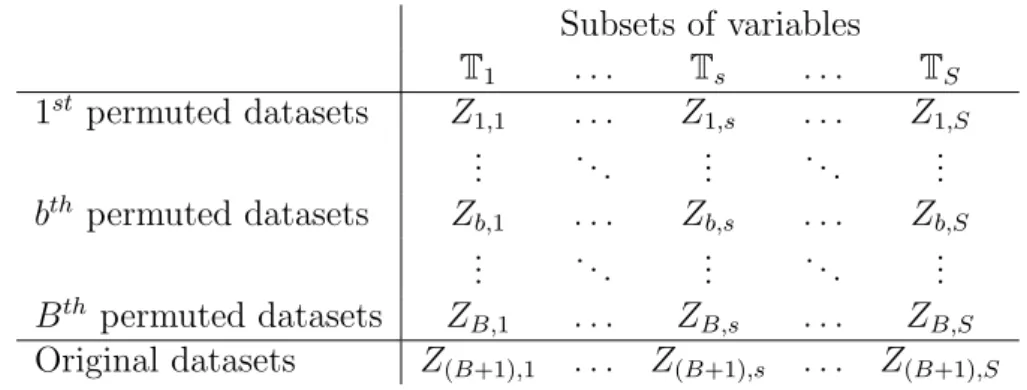
Table 2.1: Test statistics for performed tests on the B + 1 permuted datasets

re-garding the S subsets of variables.

Subsets of variables T1 . . . Ts . . . TS 1st _{permuted datasets} _Z 1,1 . . . Z1,s . . . Z1,S .. . . .. ... . .. ... bth permuted datasets Zb,1 . . . Zb,s . . . Zb,S .. . . .. ... . .. ... Bth permuted datasets ZB,1 . . . ZB,s . . . ZB,S Original datasets Z(B+1),1 . . . Z(B+1),s . . . Z(B+1),S

Table 2.2: Overview of p-values computation given the corresponding test statistic

values from Table 2.1.

Subsets of variables T1 . . . Ts . . . TS Combinant 1st _{permuted datasets} _p 1,1 . . . p1,s . . . p1,S → pC1 .. . . .. ... . .. ... ... bth permuted datasets pb,1 . . . pb,s . . . pb,S → pCb .. . . .. ... . .. ... ... Bth permuted datasets pB,1 . . . pB,s . . . pB,S → pCB Original datasets p(B+1),1 . . . p(B+1),s . . . p(B+1),S → pCB+1

to be dependent. Hence, distributions of the two combinants under the null hypothesis are unknown. One way to overcome this problem and turn out with the distributions is to resort to a permutation framework (Pesarin and Salmaso, 2010). Given the two datasets _X and _Z, new data are obtained by randomly swapping observations between the original sets. This guarantees that the distribution of the permuted samples are identical, i.e. that we are under the null hypothesis H0. Based on the permuted data,

the S tests are applied with respect to the sampled variable sets. The procedure is performed B times, and the obtained results can be collected in a table such as Table 2.1.

The results of multiple tests are specifically combined. Firstly for each test statistic value Zbs the p-value is computed by columns of Table 2.1 as

pb,s =

PB+1

k=1 1{Zb,s ≤Zk,s}

B+ 1 ,

where ₁_{·} is the identity function. In this way the analogous table of p-values is constructed (Table 2.2). Afterwards, the chosen combinants are computed by rows. Note that we obtain B + 1 combinedp-values (denoted as pC