Title
A distributionally robust joint chance constrained optimization model for the dynamic network design problem under demand uncertainty
Author(s) Sun, H; Gao, Z; Szeto, WY; Long, J; Zhao, F
Citation Networks and Spatial Economics, 2014, v. 14 n. 3-4, p. 409-433
Issued Date 2014
URL http://hdl.handle.net/10722/202639
A Distributionally Robust Joint Chance Constrained Optimization
Model for the Dynamic Network Design Problem under Demand
Uncertainty
Hua Sun • Ziyou Gao • W.Y. Szeto • Jiancheng Long • Fangxia Zhao•
Abstract This paper develops a distributionally robust joint chance constrained optimization model for a dynamic network design problem (NDP) under demand uncertainty. The major contribution of this paper is to propose an approach to approximate a joint chance-constrained Cell Transmission Model (CTM) based System Optimal Dynamic Network Design Problem with only partial distributional information of uncertain demand. The proposed approximation is tighter than two popular benchmark approximations, namely the Bonferroni’s inequality and second-order cone programming (SOCP) approximations. The resultant formulation is a semidefinite program which is computationally efficient. A numerical experiment is conducted to demonstrate that the proposed approximation approach is superior to the other two approximation approaches in terms of solution quality. The proposed approximation approach may provide useful insights and have broader applicability in traffic management and traffic planning problems under uncertainty.
Keywords Dynamic network design problem ∙ Distributionally robust joint chance
constraints ∙ Worst-case conditional value-at-risk ∙ Semidefinite programming ∙ Demand uncertainty
1 Introduction
Traditionally, dynamic transportation network design problems assume that the input data demand and parameters are deterministic. However, in reality, the input data and parameters are usually uncertain. The evaluation of network performance without accounting for the uncertainty can potentially lead to suboptimal network design
Hua Sun
MOE Key Laboratory for Urban Transportation Complex Systems Theory and Technology,Beijing Jiaotong University , Beijing 100044, China
Email: [email protected] Ziyou Gao
Institute of System Science, School of Traffic and Transportation, Beijing Jiaotong University, Beijing 100044, China
Email: [email protected]
W.Y. Szeto
Department of Civil Engineering, The University of Hong Kong, Pokfulam Road, Hong Kong, China
Email: [email protected] Jiancheng Long
School of Transportation Engineering, Hefei University of Technology, Hefei 230009, China
Email: [email protected]
Fangxia Zhao
MOE Key Laboratory for Urban Transportation Complex Systems Theory and Technology,Beijing Jiaotong University , Beijing 100044, China
decisions (Waller et al. 2001). Thus, it is of paramount importance to study the dynamic network design problem under uncertainty from a pragmatic perspective. Recently, chance-constrained programming (CCP) (Charnes et al. 1958) has been employed to formulate and analyze the dynamic NDP under uncertainty (Waller and Ziliaskopoulos 2001; Ukkusuri and Waller 2008) or the core problem of dynamic NDPs, i.e., dynamic traffic assignment (DTA), (Waller and Ziliaskopoulos 2006; Yazici and Ozbay 2010; Chung et al. 2012). In these studies, except Chung et al. (2012), the exact probability distributions of uncertainty are assumed to be known perfectly. In fact, these distributions may be unavailable (inaccurate) as we may have no (insufficient) data to calibrate the distributions, but only the partial information on the distribution, such as its first and second moments and its support, may be available. Against this background, a distributionally robust chance-constrained approach has been introduced recently to formulate and approximate DTA (Chung et al. 2012). However, the approximation for distributionally chance constraints in Chung et al. (2012) is overly conservative.
In this paper, we propose a computationally tractable and less conservative approximation method for formulating the chance-constrained system optimal dynamic network design problem based on known mean and variance of the uncertain time-dependent traffic demand, aiming to provide a robust and tractable but less conservative framework for the dynamic traffic planning and control. A numerical example is presented in this paper to illustrate the value of our less conservative approximation scheme in the context of stochastic dynamic NDPs. Moreover, computational validity is also demonstrated in the proposed framework. This paper further enriches the body of knowledge in stochastic dynamic NDPs by considering the issues in relation to the robustness, conservatism and partial distributional information.
2 Literature Review
The transportation network design problem is at the core of many transportation applications. The models and algorithms have been extensively studied in the past three decades (Boyce 1984; Magnanti and Wong 1984; Minoux 1989; Yang and Bell 1998; Chen et al. 2011). However, the vast body of previous literature has focused only on the static NDPs. Lin et al. (2011) pointed out that static NDP models cannot capture realistic, time-varying demand whereas the dynamic NDP models can. Janson (1995) and Waller (2000) revealed that the DTA-based NDP models are more desirable than the static models. In order to overcome these deficiencies, a variety of recent papers focused more on the DTA-based NDPs (Waller et al. 2006; Ukkusuri and Waller 2008; Karoonsoontawong and Waller 2006). According to Lin et al. (2011), these DTA-based NDP models can be divided into two categories: 1) single-level models and 2) bi-level models.
The single-level DTA-based NDP models are those based on the single-destination system-optimal (SO) (Ziliaskopoulos 2000) or user-optimal (UO) (Ukkusuri and Waller 2008) dynamic traffic assignment models, including the single-level SO DTA-based NDP model formulated by Waller et al. (2006) and the single-level SO DTA-based NDP model formulated by Ukkusuri and Waller (2008). The common feature of the above-mentioned single-level models is that the cell transmission model (CTM) (Daganzo 1994, 1995) is
used to model the dynamic traffic flow propagation, and the demand is assigned to the network by either the dynamic SO or UO principle. Moreover, these models are often formulated as a linear program, and therefore they are computationally tractable.
Similar to the static NDPs, the bi-level DTA-based NDPs can usually be modeled as leader-follower games, in which the transportation manager is the leader of each game who makes network design decisions and the users are the followers of the game who can freely choose their route (Boyce 1984; Yang and Bell 1998). Therefore, each of the bi-level DTA-based NDP models can be formulated as a bi-level linear program, in which the objective of the upper-level model is to minimize the total system travel time, whereas the lower-level characterizes the dynamic UO flow pattern. An example of the bi-level DTA-based NDP model is the model developed by Karoonsoontawong and Waller (2006). It is noted that although a bi-level DTA-based NDP model can be reformulated into a single-level model, the resultant formulation is a mathematical program with equilibrium constraints (MPEC) (or equivalently a mathematical program with complementarity constraints (MPCC)) rather than a linear program. Therefore, the bi-level models are more difficult to solve than the single-level models. Hence, heuristics are often developed to solve the bilevel models for general network settings. For example, Karoonsoontawong and Waller (2006) developed three meta-heuristics, namely simulation annealing, genetic algorithm, and random search, for solving the DTA-based NDPs over multi-destination large-size networks. Lin et al. (2011) and Lin (2011) further proposed two heuristic algorithms based on the Dantzig-Wolfe decomposition principle and the dual variable approximation for solving the bi-level DTA-based NDPs.
On the other hand, uncertainty is inseparable from transportation problems. For example, travel demand is uncertain. Without an explicit and rigorous recognition of the uncertainty, any transportation network development plans and policies may take on unnecessary risk and even result in misleading outcomes (Zhao and Kockelman 2002). It is therefore important to capture uncertainty in NDPs. In this regard, a variety of recent papers introduced the uncertainty in the CTM-based NDP or DTA models.
The general approaches of addressing uncertainty in CTM-based NDP or DTA studies include chance-constrained programming (CCP) (Waller and Ziliaskopoulos 2001; Waller and Ziliaskopoulos 2006; Ukkusuri and Waller 2008), two-stage stochastic linear programming with recourse (SLP2) (Waller and Ziliaskopoulos 2001; Karoonsoontawong and Waller 2007; Patil and Ukkusuri 2007; Ukkusuri and Waller 2008) and robust optimization (RO) (Karoonsoontawong and Waller 2006; Karoonsoontawong and Waller 2007; Karoonsoontawong and Waller 2010; Chung et al. 2011; Ben-Tal et al. 2011). The first two approaches have been adopted since early 20s. For example, Waller and Ziliaskopoulos (2001) applied CCP and SLP2 to formulate the single-level CTM-based SO NDP with stochastic demands. Moreover, Ukkusuri and Waller (2008) introduced the single-level UO versions of CCP and SLP2 models, and compared them with the corresponding SO versions. Yazici and Ozbay (2010) further proposed a CTM-based DTA model with probabilistic demand and road capacity constraints. Karoonsoontawong and Waller (2007) applied SLP2 to formulate the bi-level CTM-based NDPs. Karoonsoontawong and Waller (2010) further extended their previous model to incorporate the signal setting design decision. The above-mentioned CTM-based NDP
models were, however, developed by the CCP or SLP2 approach and it is necessary for the model users to know the probability distributions of the uncertain input data and parameters in order to use these models. In fact, the distributions may be unavailable (inaccurate) as we may have no (insufficient) data to calibrate the distributions. Therefore, robust optimization (Mulvey et al. 1995; Ben-Tal et al. 2009; Bertsimas et al. 2011) have been introduced recently to address the limitations of CTM-based NDPs or DTA.
According to Chung et al. (2012), robust optimization can be roughly classified into two groups: 1) scenario-based robust optimization, and 2) set-based robust optimization. The scenario-based robust optimization approach represents uncertainty via a limited number of discrete scenarios associated with strictly positive probabilities of occurrence, and attempts to solve the optimization problem across these scenarios for solutions that are near-optimal with respect to the population of all possible realizations of uncertainty (Yin et al. 2009). Mulvey et al. (1995) developed a scenario-based RO approach for general linear programming (LP) problems. Karoonsoontawong and Waller (2006) adopted this approach to propose the CTM-based NDP bi-level linear programming formulation. Karoonsoontawong and Waller (2007) adopted the same approach to formulate the CTM-based single-level SO and UO NDP models and bi-level NDP model, and made comparison with SPL2 and deterministic approaches. Ukkusuri et al. (2007) adopted the bi-level programming approach to develop a scenario-based robust discrete network design model, in which the lower-level problem is the dynamic user equilibrium problem. Karoonsoontawong and Waller (2010) later presented a scenario-based robust bi-level model for the combined network capacity expansion and signal setting design problem. Meanwhile, Mudchanatongsuk et al. (2008) pointed out that the scenario-based robust optimization approach has the following three difficulties: 1) Similar to CCP and SLP2, the scenario-based robust optimization approach also requires that the probability distribution of each scenario is known in advance; 2) the numerous scenarios used in accurately representing the uncertainty can lead to large, computationally challenging problems, and; 3) the solution obtained may be sensitive to possible uncertainty outcomes. Therefore, more attention has been paid to the set-based robust optimization approach recently.
Unlike CCP, SLP2 and the scenario-based robust optimization approach, the set-based robust optimization approach (Kouvelis and Yu 1997; Ben-Tal and Nemirovski 1998, 1999, 2000, 2002; Bertsimas and Sim 2004) does not require the assumption that the probability distributions of the uncertain input data and parameters are known. Therefore, the set-based robust optimization approach recently has not only been applied to the static NDPs (Yin and Lawpongpanich 2007, 2008; Yin et al. 2009; Lou et al. 2009; Lou et al. 2010) but also the CTM-based dynamic NDPs (Chung et al. 2011) or DTA (Yao et al. 2009). In these studies, the uncertain input data and parameters are assumed to be belonging to a bounded set. For example, Chung et al. (2011) assumed a box uncertain set for demand to formulate a single-level robust NDP model whereas Yao et al. (2009) adopted the polyhedral, box, and ellipsoid uncertain sets for demand to develop the CTM-based system-optimal DTA (SODTA) models.
The robust solutions obtained in the above-mentioned studies are, however, overly conservative. To alleviate the conservatism of the robust solutions, Ben-Tal et al. (2004)
proposed the adjustable robust optimization approach for general linear programming models. Ben-Tal et al. (2011) used the adjustable robust optimization methodology to solve the CTM-based SODTA under demand uncertainty. The polyhedral set is used as the uncertain demand set and the affinely adjustable robust counterpart (AARC) is reformulated into a linear program by using the affine control rule. Recently, a new robust optimization approach for the chance constraints has been applied to formulate CTM-based SODTA. Chung et al. (2012) developed a CTM-based SODTA model under demand uncertainty with the distributionally robust joint chance constraints. Providing that only the partial distribution information (mean and variance) was available, the distributionally robust joint chance constraints were approximated by the linear constraint based on Bonferroni’s inequality. Nevertheless, the Bonferroni’s approximation may still be overly conservative.
In this paper, a new approximation approach for the distributionally robust joint chance constraints is proposed to formulate a single-level CTM-based system-optimal NDP (SONDP) under demand uncertainty where only the partial distributional information (i.e., mean and variance) of uncertain demand is available. The single-level structure is adopted because it can provide an easier way to approximate the distributional robust joint chance constraints and makes the resultant NDP model to be computationally tractable. We develop a less conservative approximation for the distributionally robust joint chance constraints in the context of CTM-based SONDP. The distributionally robust joint chance constraints in the model are firstly approximated by the Worst-Case Conditional Value-at-Risk (WCVaR) constraints, and then the approach proposed by Zymler et al. (2013) is adopted to reformulate the WCVaR constraint into the semidefinite programming (SDP) constraint. The numerical results are provided in the latter section to illustrate the improved solution quality offered by the SDP-based approximation over the two other approximations, i.e., Bonferroni’s approximation and the approximation by Chen et al. (2010).
The remainder of this paper is structured as follows. In Section 3, we present a deterministic CTM-based SONDP formulation and reformulate it into a robust joint chance-constrained program after incorporating the uncertain demand. Section 4 presents the Worst-Case CVaR approximation and the other two approximation approaches for the robust joint chance constraints. The solution algorithm for solving the resultant program derived from the SDP and SOCP approximations is presented in Section 5. In Section 6, the numerical experimental results are presented to demonstrate the effectiveness of the proposed approach. Finally, Section 7 concludes the paper and proposes the direction for future research.
3 Deterministic and distributionally robust joint chance constraint
model
In this section, we firstly describe a deterministic CTM-based system-optimal NDP (SONDP) and then reformulate it into a robust joint chance-constrained program by introducing the uncertain demand. For ease of discussion, the notation used in these models is presented in Table 1.
Sets Description
ℑ Set of time intervals {1, 2,..., }T
C Set of cells
R
C Set of source cells
S
C Set of sink cells
A
Adjacent matrix, A={ }aij ; if cell i is connected to cell j, then aij =1,
otherwise aij =0
Parameters Description t
i
d Demand generated at cell i during time interval t, i∈CR
t i
c Travel cost associated with a vehicle in cell i during time interval t
t i
N Capacity of cell i during time interval t
t i
δ Ratio of the free-flow speed to the backward wave speed associated with cell i and time interval t
t i
Q Inflow/Outflow capacity of cell i in time interval t
ˆi
x Initial number of vehicles in cell i
Functions Description i
χ Increase in Nit for a unit increase in bi
i
φ Increase in Qit for a unit increase in bi
B Total budget
Variables Description i
b Budget spent on cell i for improvement
t i
x Number of vehicles in cell i in time interval t,
t ij
y Number of vehicles that move from cell i to cell j during time interval
t
b Vector of budgets allocated to cells, b=(...., ,...)bi x Vector of the numbers of vehicles in cells, x=(...,xit,...)
(..., ijt,...)
y= y
The CTM-based SONDP formulation aims to minimize the total cost, which is the sum of the product of the number of vehicles in each cell in each time interval and the corresponding travel cost. The travel cost of a vehicle in cell i during time interval t,
t i c , is set as follows: 1 \ , , \ , , s t i s i C C t T c M i C C t T ∈ ≠ = ∈ =
where M is assumed to be a sufficiently large positive number, which can be interpreted as the cost of a vehicle that cannot arrive at the destination by the end of time horizon. Because the penalty cost M is used in the objective function, the objective of the problem can be interpreted as minimizing the number of vehicles staying in the network by the end of the modeling horizon. By assuming a linear relationship between the budget spent on a cell and the additional capacity of that cell, the deterministic CTM-based SONDP can be formulated as the following linear program (Waller et al., 2006): SONDP: , , \ min , s t t i i x y b t i C C c x ∈ℑ ∈
∑ ∑
subject to it it 1 ki tki1 ij ijt 1 it 1 k C j C x x− a y− a y− d − ∈ ∈ − −∑
+∑
= ∀ ∈i C tR, ∈ ℑ, (1) it it 1 ki kit 1 ij ijt 1 0 k C j C x x− a y− a y− ∈ ∈ − −∑
+∑
= ∀ ∈i C C\ R∪C tS, ∈ ℑ, (2) t t ij ij i j C a y x ∈ ≤∑
∀ ∈i C C t\ S, ∈ ℑ, (3) ( ) t t t t ki ki i i i i i k C a y δ N χb x ∈ ≤ + −∑
∀ ∈i C C\ R∪C tS, ∈ ℑ, (4) t t ki ki i i i k C a y Q φb ∈ ≤ +∑
∀ ∈i C C\ R∪C tS, ∈ ℑ, (5) t t ij ij i i i j C a y Q φb ∈ ≤ +∑
∀ ∈i C C t\ S, ∈ ℑ, (6) \ , s i i C C b B ∈ ≤∑
(7) 0 ˆ i i x =x ∀ ∈i C C\ S, (8) 0 0, ij y = ∀( , )i j ∈ ×C C, (9) 0, t i x ≥ ∀ ∈i C C t\ S, ∈ ℑ, (10) 0, t ij y ≥ ∀( , )i j ∈ ×C C t, ∈ ℑ, (11) 0, i b ≥ ∀ ∈i C C\ S. (12)The objective function of SONDP represents the total travel cost, which provides an optimistic estimate or lower bound of total cost as it simplifies the original CTM model by Daganzo (1994, 1995) and allows vehicle holding. Both constraints (1) and (2) are the flow conservation constraints in cell i in time interval t. Because only the source cells generate demand, the right-hand-side of constraint (1) is set as dit−1 and the right-hand-side of constraint (2) is equal to zero. Constraint (3) bounds the total outflow rate of a cell by its current occupancy. Constraint (4) ensures that the total inflow rate of a cell is bounded by its remaining capacity. Constraints (5) and (6) state that the total inflow into and outflow rate from a cell are limited by the inflow and outflow capacities respectively. Constraint (7) is a budgetary constraint. The remaining constraints (8) to (12) represent the initial conditions and non-negativity conditions.
As the problem is a minimization problem and constraint (1) is the only set of constraints related to demand generation, constraint (1) can be reformulated into the following inequality constraint (Waller and Ziliaskopoulos 2006, Chung et al. 2012):
1 1 1 1 , , . t t t t t i i ki ki ij ij i R k C j C x x− a y− a y− d − i C t ∈ ∈ − −
∑
+∑
≥ ∀ ∈ ∈ ℑ (13)This model allows vehicle holding (Doan and Ukkusuri, 2012) because constraint (13) is always binding and equation (1) and constraint (13) are equivalent. When we incorporate the uncertain demand into the deterministic CTM-based SONDP model, we reformulate constraint (13) into the following joint chance constraint (14) with a confidence parameter ε∈(0,1): it it 1 ki kit 1 ij ijt 1 it 1 R, , k C j C x x− a y− a y− d − i C t ε ∈ ∈ − − + ≥ ∀ ∈ ∈ ℑ ≥
∑
∑
P (14)where dit−1 denotes the random demand variable. The violation of constraint (14) implies that more demand is realized than is used for prediction. According to the assumption that the only partial distribution information of uncertain demand may be available, the joint chance constraint (14) can be reformulated as follows:
1 1 1 1 Inf it it ki kit ij ijt it R, , k C j C x x− a y− a y− d − i C t ε ∈ ∈ ∈ − − + ≥ ∀ ∈ ∈ ℑ ≥
∑
∑
P PP (15)where P denotes the set of all probability distributions that are consistent with the know mean and variance of uncertain demand. Then, the CTM-based SONDP with the distributionally robust joint chance constraints can be rewritten as:
SONDP-RJCCP: , , \ min , s t t i i x y b t i C C c x ∈ℑ ∈
∑ ∑
subject to constraints (2)-(12) and (15).
4 Approximation of distributionally robust joint chance constraints
In this section, we start with using the approximation approach based on semidefinite programming (SDP) proposed by Zymler et al. (2013) to approximate the distributionally robust joint chance constraint (15), and then present the two benchmark approximations
of constraint (15). One approximation is based on Bonferroni’s inequality and the other is based on second-order conic programming (SOCP) (Chen et al. 2010). Finally, we compare the three approximations for the distributionally robust joint chance constraints.
4.1
The Worst-Case Conditional Value-at-Risk approximation
Assume that the uncertain demand depends affinely on a random number ξ ∈1, i.e.,
t t t
i i i
d =µ σ ξ+ , where µit and (σit)2 are denoted as the mean and variance of the demand, respectively. The mean and variance of the random number ξ are, respectively, assumed to be 0 and 1, i.e.,E( )ξ =0,and Var( )ξ =1. For notation purposes, we let the following be the second-order moment matrix ofξ:
( ) ( ) ( ) 1 0 ( ) 1 0 1 Var E E E ξ ξ ξ ξ + Ω = = .
Based on the above setting, Chen et al. (2010) proved that the joint chance constraint (15) can be reformulated into
1 1 1 1 1 , Inf max 0 R t t t t t t t i i i ki ki ij ij i i i C t k C j C x x a y a y α − − − µ − σ ξ− ε ∈ ∈ ∈ℑ ∈ ∈ − + − + + ≤ ≥
∑
∑
P P P , (16) where | | | | { t| CR , (..., t,...) 0} i i α∈ = α α∈ × ℑ α = α >A is called the scaling parameter. The
choice of α∈A does not affect the feasible region of the chance constraint (15). Although these scaling parameters are seemingly redundant, it turns out that they can be tuned to improve the quality of approximation. Chen et al. (2010) indicated that constraint (16) represents a distributionally robust individual chance constraint, which can be approximated by a Worst-Case CVaR constraint. Thus, the feasible region of constraint (15) can be approximated by
1 1 1 1 1
1 ,
( ) ( , ) : sup CVaR max 0 ,
R t t t t t t t i i i ki ki ij ij i i i C t k C j C x y ε x x a y a y α α − − − µ− σ ξ− − ∈ ∈ℑ ∈ ∈ ∈ = − + − + + ≤ P P
∑
∑
Z (17) Where 1 1 1 1 1 1 , CVaR max R t t t t t t t i i i ki ki ij ij i i i C t k C j C x x a y a y ε α − − − µ − σ ξ− − ∈ ∈ℑ ∈ ∈ − + − + + = ∑
∑
1 1 1 1 1 , 1 inf max . 1 R t t t t t t t i i i ki ki ij ij i i i C t k C j C x x a y a y β β ε α µ σ ξ β + − − − − − ∈ ∈ ∈ℑ ∈ ∈ + − + − + + − − ∑
∑
P R E (18) β is a decision variable in the chance constraint; EP( ) denotes the expectation withrespect to P, and ( )• =+ max
{ }
•, 0 (Rockafellar and Uryasev 2000, 2002). In contrast to the chance constraint (16), ( , )x y ∈Z( )α depends on the choice of α∈A . Because the max function in constraint (16) is not concave, the Worst-Case CVaR constraint (17) is not equivalent to constraint (16) (Chen et al. 2010).Zymler et al. (2013) developed an approximation approach for distributionally robust chance constraints based on semidefinite programming (SDP). The first- and second-order moments with the supports of uncertain parameters are assumed to be known. Zymler et al. (2013) firstly approximated the distributionally chance constraints by the Worst-case Conditional Value-at-Risk (WCVaR) constraints, and then reformulated the WCVaR constraints into the SDP constraints using the theory of moment problems and conic duality arguments. They argued that this approximation is exact for robust individual chance constraints with concave or quadratic constraint functions and this approximation is tighter than the two other benchmark approximations for robust joint chance constraints. In this study, we adopt their approach to approximate constraint (15) and present the following theorem about the equivalent form of constraint (17).
Theorem 1: If dit−1 follows an unknown probability distribution with the mean µit−1 and variance (σit−1 2) , then the distributionally robust joint chance constraint (15) can be approximated by the following semidefinite programming constraint:
2 1 1 1 1 1 1 ( , ) 1 , 0, 0 1 ( ) ( , ) : , , , 0 / 2 0 / 2 ( ) R t t i i t t t t t t t t i i i i i ki ki ij ij i k C j C MM MM MM x y i C t MM x x a y a y β β ε α α σ α σ α µ β − − − − − − ∈ ∈ ∃ ∈ × + Ω ≤ − = ∀ ∈ ∈ℑ − − + − + −
∑
∑
Z R S ± ± (19) where S2 denotes the space of real symmetric matrices of dimension two,, ( )
A B =trace AB is a trace scalar product of matrices A and B, and A± 0 means that
the matrix A is semidefinite.
Proof: We note that constraint (17) is equivalent to J x y( , , )α ≤0, where
1 1 1 1 1
1
,
( , , ) sup CVaR max
R t t t t t t t i i i ki ki ij ij i i i C t k C j C J x y α −ε α x− x a y− a y− µ − σ ξ− ∈ ∈ℑ ∈ ∈ ∈ = − + − + +
∑
∑
P P 1 1 1 1 1 , 1sup inf max .
1 R t t t t t t t i i i ki ki ij ij i i i C t k C j C x x a y a y β β ε α µ σ ξ β + − − − − − ∈ ∈ ∈ℑ ∈ ∈ ∈ = + − − + − + + −
∑
∑
P R P E P(20) According to the stochastic saddle point theorem (Shapiro and Kleywegt, 2002), we can interchange the maximization and minimization operations as below:
1 1 1 1 1
,
1
( , , ) inf sup max .
1 R t t t t t t t i i i ki ki ij ij i i i C t k C j C J x y x x a y a y β α β α µ σ ξ β ε + − − − − − ∈ ∈ ∈ ∈ℑ ∈ ∈ = + − − + − + + −
∑
∑
P R P P E (21) Next, we derive the dual problem of the following Worst-Case expectation problem:1 1 1 1 1 , sup max R t t t t t t t i i i ki ki ij ij i i i C t k C j C x x a y a y α µ σ ξ β + − − − − − ∈ ∈ℑ ∈ ∈ ∈ − + − + + −
∑
∑
P P E P . (22)Using Lemma 1 in Zymler et al. (2013), we have:
2 inf , , MM MM ∈S Ω (23) subject to
[ ]
[ ]
1 1 1 1 1 , ,1 ,1 max , R T t t t t t t t i i i ki ki ij ij i i i C t k C j C MM x x a y a y ξ ξ α − − − µ− σ ξ− β ∈ ∈ℑ ∈ ∈ ≥ − + − + + − ∑
∑
∀ ∈ξ , (24) 0. MM ± (25) We note that the above optimization problem represents a lossless reformulation of the worst-case expectation problem (22). The semi-infinite constraint (24) can be expanded into |CR| |× ℑ| simpler semi-infinite constraints in the form of[ ]
[ ]
1 1 1 1 1 ,1T ,1 it it it ki kit ij ijt it it , R, , . k C j C MM x x a y a y i C t ξ ξ α − − − µ − σ ξ− β ξ ∈ ∈ ≥ − + − + + − ∀ ∈ ∈ ℑ ∈ ∑
∑
(26) Constraint (26) can be equivalently expressed as1 1 1 1 1 1 0 / 2 0, , . / 2 ( ) t t i i t t t t t t t t R i i i i i ki ki ij ij i k C j C MM x x a y a y i C t α σ α σ α µ β − − − − − − ∈ ∈ − − + − + − ∀ ∈ ∈ ℑ
∑
∑
± (27) Therefore, ( , , ) inf + 1 , , 1 J x y MM β α β ε ∈ = Ω − (28) subject to MM∈S2, MM ± 0, 1 1 1 1 1 1 0 / 2 0, , . / 2 ( ) t t i i t t t t t t t t R i i i i i ki ki ij ij i k C j C MM x x a y a y i C t α σ α σ α µ β − − − − − − ∈ ∈ − − + − + − ∀ ∈ ∈ ℑ ∑
∑
±Thus, the claim follows. ■
formulated as follows. SDP model: , , , \ min , s t t i i x y b t i C C c x α
∑ ∑
∈ℑ ∈ subject to J x y( , , )α ≤0, (29) constraints (2)-(12).4.2 The Bonferroni Approximation
A popular approximation for constraint (15) is based on Bonferroni’s inequality. We note that constraint (15) is equivalent to the following:
1 1 1 1 Inf ,it it ki tki ij ijt it R, k C j C x x− a y− a y− d − i C t ε ∈ ∈ ∈ − − + ≥ ∀ ∈ ∈ ℑ ≥
∑
∑
P P P 1 1 1 1 , sup 1 . R t t t t t i i ki ki ij ij i i C t k C j C x x− a y− a y− d − ε ∈ ∈ℑ ∈ ∈ ∈ ⇔ − − + < ≤ − ∑
∑
P P P (30)Moreover, according to Chung et al. (2012), Bonferroni’s inequality implies that
1 1 1 1 , R t t t t t i i ki ki ij ij i i C t k C j C x x− a y− a y− d − ∈ ∈ℑ ∈ ∈ − − + < ≤
∑
∑
P 1 1 1 1 , , R t t t t t i i ki ki ij ij i i C t k C j C x x− a y − a y− d − ∈ ∈ℑ ∈ ∈ − − + < ∀ ∈ ∑
P∑
∑
P P. (31) Thus, we have 1 1 1 1 , Inf it it ki kit ij ijt it 0 1 i t, R, , k C j C x− x a y− a y− d − ε i C t ∈ ∈ ∈ − + − + ≤ ≥ − ∀ ∈ ∈ ℑ ∑
∑
P P P (32)where the confidence level εi t, is required to satisfy the constraint , , 1
R i t
i C∈ t∈ℑε ≤ −ε
∑
.Therefore, constraint (32) represents the conservative approximation for constraint (15). A major limitation of the Bonferroni approximation is that the approximation quality critically depends on the choice of confidence level εi t, . Unfortunately, the problem of finding the best εi t, for constraint (15) is nonconvex and it is believed to be intractable (Nemirovski and Shapiro 2006). According to Nemirovski and Shapiro (2006), we set
, 1 | | | | i t R C ε ε = −
× ℑ , where |CR| is the number of source cells and |ℑ| denotes the number of discrete time intervals. Thus, constraint (32) can be reformulated into the linear constraint as follows (Calafiore and Ghaoui 2006; Chung et al. 2012):
1 1 1 1 1 | | | | + 1 0 , , 1 t t t t t t R i i ki ki ij ij i i R k C j C C x x a y a y µ σ i C t ε − − − − − ∈ ∈ × ℑ − + − + − ≤ ∀ ∈ ∈ ℑ −
∑
∑
. (33)Thus, the approximated SONDP-RJCCP can be formulated as following LP model: LP model: , , \ min , s t t i i x y b t i C C c x ∈ℑ ∈
∑ ∑
subject to constraints (2)-(12) and (33).
As shown in the above formulation, the model is still an LP model and can be computed efficiently. However, the Bonferroni approximation is overly conservative. Zymler et al. (2013) proved that the accuracy of the Bonferroni approximation diminishes with an increasing number of joint constraints if the inequalities in the joint chance constraints are positively correlated.
4.3 The approximation by Chen et al. (2010)
To minimize the over-conservatism of the Bonferroni approximation, Chen et al. (2010) proposed an approximation approach for the robust joint chance constraints based on second-order cone programming (SOCP) by using inequalities from the probability theory. Moreover, they also proved that their approximation is tighter than the Bofferroni approximation. In this subsection, we adopt their results to approximate constraint (15). Similar to the Worst-Case CVaR approximation, according to the above discussion, the robust joint constraint (15) can be approximated by
1 1 1 1 1
1 ,
ˆ ( ) ( , ) : sup CVaR max 0 ,
R t t t t t t t i i i ki ki ij ij i i i C t k C j C x y ε x x a y a y α α − − − µ− σ ξ− − ∈ ∈ℑ ∈ ∈ ∈ = − + − + + ≤ P
∑
∑
Z P (34) where 1 1 1 1 1 1 ,sup CVaR max
R t t t t t t t i i i ki ki ij ij i i i C t k C j C x x a y a y ε α − − − µ − σ ξ− − ∈ ∈ℑ ∈ ∈ ∈ − + − + +
∑
∑
P P 1 1 1 1 1 , 1inf sup max .
1 R t t t t t t t i i i ki ki ij ij i i i C t k C j C x x a y a y β β ε α µ σ ξ β + − − − − − ∈ ∈ ∈ ∈ℑ ∈ ∈ = + − − + − + + −
∑
∑
P R P P EChen et al. (2010) employed the results of Chen and Sim (2009) to provide an upper bound of EP
( )
[ ]
• + . Thus, constraint (34) can be approximated by the following SOCP (Chen et al. 2010): ˆ( , , ) 0, J x y α ≤ (35) where 0 0 , 1 ˆ( , , ) min min ( , ) 1 w w J x y w w β α β π β ε ∈ ∈ = + − − R R 1 1 1 1 0 1 , 1 ( ) , 1 R t t t t t t t t i i i ki ki ij ij i i i i C t k C j C x x a y a y w w π α µ α σ ε − − − − − ∈ ∈ℑ ∈ ∈ + − + − + − − − ∑
∑
∑
(36) and( )
0 0( )
0 2 1 1 , , . 2 2 z z z z z π = + (37)problem which can be formulated as follows. SOCP model: , , , \ min , s t t i i x y b t i C C c x α
∑ ∑
∈ℑ ∈subject to constraints (2)-(12) and (35).
It is noted that similar to the Bonferroni approximation, the approximation proposed by Chen et al. (2010) critically depends on the choice of α, and that the problem of finding the best α for the robust joint chance constraint is nonconvex and therefore believed to be intractable.
5 Solution algorithm
We adopted the solution algorithm proposed by Chen et al. (2010) to solve the previous SDP and SOCP models. By Theorem 1, the original SONDP-RJCCP can be written as
SDP: , , , \ min , s t t i i x y b t i C C c x α
∑ ∑
∈ℑ ∈ subject to J x y( , , )α ≤0, constraints (2)-(12).Unfortunately, Zymler et al. (2013) proved that the Worst-Case CVaR functional
( , , )
J x y α in constraint (29) is merely biconvex, but not jointly convex in ( , )x y and
α , and hence the SDP model is nonconvex. However, when the scaling parameters α are fixed, the problem becomes convex and tractable.
To explain the preceding point, we define the set
, : 1, , , R t t i R i i C t i C t M α α α ∈ ∈ℑ = ≥ ∀ ∈ ∈ ℑ =
∑
A = , where M is a large number. Obviously,
unlike A , the set A = is closed. When α∈A = is fixed, the SDP problem is reduced to: SDP1: , , \ min , s t t i i x y b t i C C c x ∈ℑ ∈
∑ ∑
(38) subject to J x y( , , )α ≤0, constraints (2)-(12).SDP1 is equivalent to a tractable SDP problem and the feasible solution of SDP1 is also feasible to the SONDP-RJCCP.
Chen et al. (2010) proposed an algorithm to improve the objective value by tuning the scaling parameters α . Consequently, they introduce the following tractable SDP problem where ( , )x y is fixed:
SDP2: min ( , , ),J x y
α α (39)
subject to α∈A. (40)
feasibility of * * *
( ,x y b, ) to SDP1, it is found that * *
( , , ) 0
J x y α ≤ . If * *
( ,x y ) is fixed, then the optimal scaling parameters α*
corresponding to * *
( ,x y ) can be obtained by solving SDP2. Then, we have
* * * * *
( , , ) ( , , ) 0.
J x y α ≤J x y α ≤ (41)
This inequality implies that the optimal objective value of SDP1 with the input α*
is not larger than * \ s t t i i t i C C c x ∈ℑ ∈
∑ ∑
. Thus, a sequence of monotonically decreasing objective values can be obtained by solving SDP1 and SDP2 in alternation. This method depends on the availability of an initial feasible solution (xinit,yinit,binit) to SDP1. The following is the procedure of their algorithm, referred to as Algorithm 5.1.Algorithm 5.1
Step 1: Let (xinit,yinit,binit) be a feasible solution of problem SDP1. Set the iteration
number n←1, the current solution to (x y b0, 0, 0)←(xinit,yinit,binit) and the current
objective function to 0 0 \ s t t i i t i C C f c x ∈ℑ ∈ ←
∑ ∑
.Step 2: Solve problem SDP2 with the input (xn−1,yn−1) and obtain the optimal scaling
parameters α*. Set αn ←α*.
Step 3: Solve problem SDP1 with the input αn and obtain the optimal solution
* * * ( ,x y b, ). Setxn ←x*, yn ← y* and \ s n t t n i i t i C C f c x ∈ℑ ∈ ←
∑ ∑
.Step 4: If (fn− fn−1) / fn−1 ≤γ (where γ is a given small tolerance), then stop and
output (xn,y bn, n). Otherwise, set n← +n 1 and return to step 2.
Zymler et al. (2013) proved that the objective values {fn} generated by Algorithm
5.1 is monotonically decreasing sequence if (xinit,yinit,binit) is feasible to SDP1 for some α∈A. They also proved that if the feasible region of constraints (2)-(12) is bounded, then the sequence (xn,yn) is bounded while the sequence {fn} converges to a finite limit. Zymler et al. (2013) indicated that Algorithm 5.1 does not necessarily obtain a global optimal solution to the SDP and SOCP models. However, the methods can perform well in practice. In the next section, we will confirm this point by presenting the numerical results.
6 Numerical example
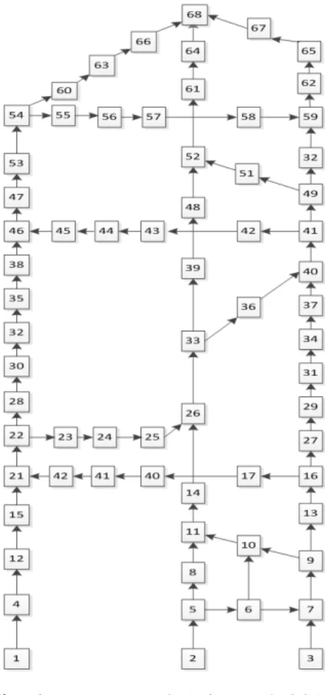
The purpose of presenting the numerical example in this section is twofold: 1) to demonstrate the effectiveness of the Worst-Case CVaR approximation for distributionally robust joint chance constraints; and 2) to illustrate the advantage of the Worst-Case CVaR approximation approach by comparing with the two other approximation approaches. Under the assumption that the mean and variance of the uncertain demands is known, an example network shown in Figure 1 is selected to test the aforementioned approaches. This cell network is composed of 68 cells and 74 cell connectors. There are three source cells (cells 1, 2, 3) and one sink cell (cell 68). The cells in the center represent the freeway, while the outer and cross cells represent arterial streets. Except the sink cell (cell 68), all cells are considered for capacity expansion. The characteristics of the cells in the test network are shown in Table 2.
Fig. 1 Test network (Lin et al. 2011)
We assume that the length of a time interval is 1s, the planning horizon is 30s and M = 10. The parameters and are assumed to be unity, i.e.,
The mean and variance of the demand are assumed to equal four and one, respectively,
i.e., . All second-order cone programs and
semidefinite programs arising from the approximation by Chen et al. (2010) and the Worst-Case CVaR approximation were, respectively, solved by using Matlab 7.11 with
the SeDuMi solver (Sturm 1999) and the YALMIP interface (Löfberg 2004), and the linear programs arising from the Bonferroni approximation was solved by Matlab 7.11 with the GLPK solver and the YALMIP interface (Löfberg 2004).
Table 2 Characteristic of the cells
Cell Nit Qit χi xˆi 1, 3 ∞ ∞ 1 0 2 ∞ 12 1 0 68 ∞ ∞ 1 0 Freeway Cell 20 12 1 0 Arterial Cell 10 8 1 0
Table 3 presents the optimal budget allocations obtained by solving the CTM-based SONDP under the three approximations when ε =90% and B=50. This table clearly shows that the total budget is allocated to each cell non-uniformly no matter which approximation method is used. Table 4 describes the optimal objective values and the percentage improvements of the objective values obtained by the SDP approximation relative to the corresponding values obtained by the LP and SOCP approximations under different confidence levels and B=50. As expected, the optimal objective value obtained by each of the three approximations increases with ε because the joint chance constraint becomes more conservative as ε grows. Moreover, the percentage improvements of the objective values obtained by the SDP approximation relative to those obtained by the LP and SOCP approximations increases with the confidence level
ε. When the confidence level ε approaches 99%, the SDP approximation outperforms the LP approximation by up to 87% and the SOCP approximation by up to 0.65%. Moreover, for the same conference level, the SDP approximation yields a smaller optimal objective value than the SOCP approximation, which in turns yields a smaller optimal objective value than the LP approximation.
Table 4 also reports the runtimes required by solving the mathematical programs derived from different approximations. It is obvious to notice that for a fixed conference level, the runtime for solving a linear programs is shorter than that for solving the corresponding second-order cone program, which in turn is shorter than that for solving the corresponding semidefinite program. It is because the problem structure of an LP problem is simpler than that of the corresponding SOCP problem, which is in turn simpler than and that of the corresponding SDP problem. This and the previous observations imply that the improved solution quality offered by the SDP approximation is obtained at the cost of longer computing time.
Table 5 shows the optimal objective values and the percentage improvements of the objective values obtained by the SDP approximation relative to the corresponding values obtained by the LP and SOCP approximations under the different budgets and ε =0.9. It
can be seen that the optimal objective value obtained by each of the three approximations decreases when the budget increases. It is because the feasible region of the CTM-based SONDP becomes larger as B grows. The two percentage improvements also increase when the budget B increases. When the budget B approaches 70, the SDP approximation outperforms the LP approximation by up to 85%, and the SOCP approximation by up to 0.27%.
Table 3 Optimal budget allocations to cells obtained by the CTM-based SONDP under the LP, SOCP, and SDP approximations when ε =90% and B=50.
Cell number LP SOCP SDP
7 0 1.156 1.167 9 0 1.156 1.167 10 0 1.156 1.167 11 5.556 5.170 5.167 14 5.556 5.170 5.167 26 5.556 5.170 5.167 33 5.556 5.170 5.167 39 5.556 5.170 5.167 48 5.556 5.170 5.167 52 5.556 5.170 5.167 61 5.556 5.170 5.167 64 5.556 5.170 5.167
Table 4 The optimal objective values of the CTM-based SONDP under the LP, SOCP, and SDP approximations when B=50
ε
(%)
Optimal objective value LP SDP
LP − (%) SOCP SDP SOCP − (%) Runtime LP SOCP SDP LP SOCP SDP 50 31521.5361 6540.5259 6530.0127 79.28 0.1673 352.6791 764.3291 801.1855 60 34836.3225 6877.0969 6865.3323 80.29 0.1710 348.9165 776.4275 827.3901 70 39690.8952 7333.1484 7319.3851 81.56 0.1877 360.7921 791.4784 863.2471 80 47829.9268 8125.9495 8107.3500 83.05 0.2289 367.2473 805.2914 882.9713 90 66191.1903 10071.9018 10044.3549 84.83 0.2737 373.9417 823.3451 905.4637 95 92147.7268 12798.5914 12759.6528 86.15 0.3042 380.6743 834.9186 917.7215 99 201660.0676 24521.7782 24361.4188 87.92 0.6539 392.8234 855.1674 976.2471
Table 5 The optimal objective values of the CTM-based SONDP under the LP, SOCP, and SDP approximations when ε =90%
B
Optimal objective value LP SDP
LP − (%) SOCP SDP SOCP − (%) Runtime LP SOCP SDP LP SOCP SDP 10 66831.1903 10631.1680 10603.0215 84.13 0.2648 350.8145 712.2156 767.1963 20 66671.1903 10472.8361 10444.7993 84.33 0.2677 374.9885 724.4762 771.8935 30 66511.1903 10321.7046 10293.6882 84.52 0.2714 383.2667 735.6738 782.4568 40 66351.1903 10185.2395 10157.6882 84.69 0.2705 397.2521 750.2473 789.3479 50 66191.1903 10071.9242 10044.3549 84.83 0.2737 412.9876 776.5429 801.1855 60 66031.1903 9958.5447 9931.0215 84.96 0.2764 434.3687 789.4792 824.5733 70 65871.1903 9845.2362 9817.6882 85.10 0.2798 474.2434 803.3567 851.8935
To compare the operating behaviors of the optimal solutions for the three approximations, we randomly generated 100 travel demand vectors, in which the demand of each O-D pair is uniform distributed between 4− 3 and 4+ 3. For each random demand vector, the optimal objective values associated with the optimal capacity expansion plans for the three approximations were computed. The mean, standard deviation, and maximum values of the optimal objective values were generated from the simulation experiment. The results are shown and compared in Table 6. It can be seen that the mean, standard deviation, and maximum of the optimal objective values obtained by the Bonferroni (LP) approximation remain unchanged for all confidence levels. This is because that the optimal solutions of Bonferroni approximation are the same under the different confidence levels. Moreover, the mean, standard deviation, and maximum of the optimal objective values obtained by the approximation by Chen et al. (2010) (i.e., the SOCP approximation) and the Worst-Case CVaR approximation (i.e., the SDP approximation) increase with the confidence level ε. This is also because that the joint chance constraints become less restrictive as ε grows. However, the mean, standard deviation, and maximum of the optimal objective value under the Worst-Case CVaR approximation outperforms the two other approximations. It is continuing to show that the Worst-Case CVaR approximation is less conservative. In addition, when the confidence level ε increases to a threshold level, the three approximations yield the same mean, standard deviation and maximum of the optimal objective because the optimal solutions for the three approximations are equal.
Table 6 Simulation results of numerical example
ε Mean Standard Deviation Maximum
LP SOCP SDP LP SOCP SDP LP SOCP SDP
10
B=
0.6 5229.6119 5225.8138 5224.8386 153.6227 153.2804 153.2760 5606.2974 5602.1704 5601.1064 0.7 5229.6119 5228.7442 5228.1800 153.6227 153.3224 155.3129 5606.2974 5604.4764 5602.3707 0.8 5229.6119 5229.6119 5229.6119 153.6227 153.6227 153.6227 5606.2974 5606.2974 5606.2974 0.9 5229.6119 5229.6119 5229.6119 153.6227 153.6227 153.6227 5606.2974 5606.2974 5606.2974 0.95 5229.6119 5229.6119 5229.6119 153.6227 153.6227 153.6227 5606.2974 5606.2974 5606.2974 0.99 5229.6119 5229.6119 5229.6119 153.6227 153.6227 153.6227 5606.2974 5606.2974 5606.2974 20 B= 0.5 5210.0316 5200.4858 5200.3416 151.3377 149.8323 149.8181 5582.9654 5569.8614 5569.6304 0.6 5210.0316 5203.2916 5202.0731 151.3377 150.2773 150.2498 5582.9654 5575.1294 5574.8434 0.7 5210.0316 5206.8949 5205.9276 151.3377 150.7059 150.6093 5582.9654 5580.5474 5579.5894 0.8 5210.0316 5209.5312 5208.5483 151.3377 151.3260 151.3159 5582.9654 5582.7604 5581.7864 0.9 5210.0316 5210.0316 5210.0316 151.3377 151.3377 151.3377 5582.9654 5582.9654 5582.9654 0.95 5210.0316 5210.0316 5210.0316 151.3377 151.3377 151.3377 5582.9654 5582.9654 5582.9654 0.99 5210.0316 5210.0316 5210.0316 151.3377 151.3377 151.3377 5582.9654 5582.9654 5582.9654 30 B= 0.5 5193.5155 5182.6046 5182.5076 148.5266 146.1546 146.1342 5560.1585 5542.8488 5542.6398 0.6 5193.5155 5190.4235 5190.2698 148.5266 147.8264 147.7942 5560.1585 5556.6945 5556.4475 0.7 5193.5155 5191.2481 5190.3737 148.5266 147.9351 147.8379 5560.1585 5558.0589 5557.0989 0.8 5193.5155 5192.2688 5191.2938 148.5266 148.1455 148.0500 5560.1585 5559.3389 5558.3789 0.9 5193.5155 5193.5155 5193.5155 148.5266 148.5266 148.5266 5560.1585 5560.1585 5560.1585 0.95 5193.5155 5193.5155 5193.5155 148.5266 148.5266 148.5266 5560.1585 5560.1585 5560.1585 0.99 5193.5155 5193.5155 5193.5155 148.5266 148.5266 148.5266 5560.1585 5560.1585 5560.1585 40 B= 0.5 5180.8740 5172.0522 5172.0101 145.7070 142.9784 142.9637 5549.7958 5528.7775 5528.7295 0.6 5180.8740 5176.0302 5175.9367 145.7070 144.3672 144.3426 5549.7958 5532.8504 5532.7384 0.7 5180.8740 5177.4635 5176.2974 145.7070 144.6887 144.6515 5549.7958 5540.5148 5539.2448 0.8 5180.8740 5178.5191 5177.5539 145.7070 145.1691 145.0771 5549.7958 5544.4868 5543.5448 0.9 5180.8740 5180.4647 5179.4983 145.7070 145.6553 145.3628 5549.7958 5549.4688 5548.5480 0.95 5180.8740 5180.8740 5180.8740 145.7070 145.7070 145.7070 5549.7958 5549.7958 5549.7958 0.99 5180.8740 5180.8740 5180.8740 145.7070 145.7070 145.7070 5549.7958 5549.7958 5549.7958 50 B= 0.5 5172.7950 5151.2526 5150.9999 143.2113 140.3553 140.5882 5529.3615 5524.4337 5523.5655 0.6 5172.7950 5168.3943 5168.3544 143.2113 141.5858 141.5655 5529.3615 5526.1495 5526.0975 0.7 5172.7950 5170.1610 5169.8288 143.2113 142.4167 142.0926 5529.3615 5526.3135 5526.2495 0.8 5172.7950 5171.1289 5170.8262 143.2113 142.9165 142.7945 5529.3615 5527.4928 5526.5288 0.9 5172.7950 5172.3447 5171.3646 143.2113 143.0314 142.9383 5529.3615 5528.9916 5528.0096 0.95 5172.7950 5172.7950 5172.7950 143.2113 143.2113 143.2113 5529.3615 5529.3615 5529.3615 0.99 5172.7950 5172.7950 5172.7950 143.2113 143.2113 143.2113 5529.3615 5529.3615 5529.3615
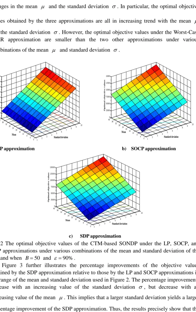
To illustrate the effect of the means and standard deviations of the uncertain demand on the optimal objective function values under the three approximations, Figure 2 is plotted. The mean and standard deviation of the uncertain demand were set in the range between 4 and 40 and between 1 and 10, respectively and B=50 and ε =90%. Figure 2 clearly depicts the
sensitivity of the optimal objective values obtained under the three approximations to the changes in the mean µ and the standard deviation σ . In particular, the optimal objective values obtained by the three approximations are all in increasing trend with the mean µ and the standard deviation σ. However, the optimal objective values under the Worst-Case CVaR approximation are smaller than the two other approximations under various combinations of the mean µ and standard deviation σ.
1 2 3 4 5 6 7 8 9 10 0 4 8 12 16 20 24 28 32 36 40 0 100000 200000 300000 400000 500000 600000 700000 800000 Standard deviation Mean O p t i m al ob j e c t i ve val u e s 1 2 3 4 5 6 7 8 9 10 0 4 8 12 16 20 24 28 32 36 40 0 25000 50000 75000 10000 12500 15000 Standard deviation Mean O p t i m al ob j e c t i ve val u e s
(a) LP approximation b) SOCP approximation
1 2 3 4 5 6 7 8 9 10 0 4 8 12 16 20 24 28 32 36 40 0 25000 50000 75000 100000 125000 150000 Standard deviation Mean O p t im al ob j e c t ive val u e s c) SDP approximation
Fig 2 The optimal objective values of the CTM-based SONDP under the LP, SOCP, and SDP approximations under various combinations of the mean and standard deviation of the demand when B=50 and ε =90%.
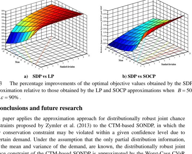
Figure 3 further illustrates the percentage improvements of the objective values obtained by the SDP approximation relative to those by the LP and SOCP approximations in the range of the mean and standard deviation used in Figure 2. The percentage improvements increase with an increasing value of the standard deviation σ , but decrease with an increasing value of the mean µ. This implies that a larger standard deviation yields a larger percentage improvement of the SDP approximation. Thus, the results precisely show that the
Worst-Case CVaR approximation is more robust and less conservative. 1 2 3 4 5 6 7 8 9 10 0 4 8 12 16 20 24 28 32 36 40 30% 35% 40% 45% 50% 55% 60% 65% 70% 75% 80% 85% 90% Standard deviation Mean R el a t iv e I m p ro v em en t b et w een L P a n d S D P 1 2 3 4 5 6 7 8 9 10 0 4 8 12 16 20 24 28 32 36 40 0 0.05% 0.1% 0.15% 0.2% 0.25% 0.3% 0.35% 0.4% 0.45% 0.5% Standard deviation Mean R e la t iv e I m pr o v e m e nt be t w e e n SO C P a nd SD P a) SDP vs LP b) SDP vs SOCP
Fig 3 The percentage improvements of the optimal objective values obtained by the SDP approximation relative to those obtained by the LP and SOCP approximations when B=50
and ε =90%.
6 Conclusions and future research
This paper applies the approximation approach for distributionally robust joint chance constraints proposed by Zymler et al. (2013) to the CTM-based SONDP, in which the flow conservation constraint may be violated within a given confidence level due to uncertain demand. Under the assumption that the only partial distribution information, i.e., the mean and variance of the demand, are known, the distributionally robust joint chance constraint of the CTM-based SONDP is approximated by the Worst-Case CVaR constraint, and then reformulated the resultant constraint into the SDP constraint by using the theory of moment problems and conic duality. This paper also presents the two other benchmark approximation approaches and compared the Worst-Case CVaR approximation approach with them. The numerical experiment shows that the Worst-Case CVaR approximation approach outperforms the other two approximation approaches in terms of solution quality.
There are some possible further research directions. Firstly, the classic cell-based SONDP exists holding-back phenomenon (Doan and Ukkusuri, 2012) which may be unrealistic. The Worst-Case CVaR approximation can be applied to the alternative deterministic mathematical formulation (Zhu and Ukkusuri, 2013) to overcome this problem. Secondly, the classic cell-based SONDP only considers demand uncertainty. One possible extension is to replace the CTM by the stochastic CTM (Sumalee et al. 2011) to consider both demand and supply uncertainties and to develop an approximation approach. Thirdly, the Worst-Case CVaR approximation has only been applied to the studied SONDP, which is a single-level optimization problem. How to apply Worst-Case CVaR approximation to the dynamic user equilibrium NDP is another challenging research direction because the problem is bi-level by nature. Lastly, the assumption that the mean and variance of the demand are known can be relaxed. The approach proposed by Delage and Ye (2010) may be used to solve the CTM-based NDP when the mean and variance of the demand are unknown but bounded.