July 2008, Volume 27, Issue 4. http://www.jstatsoft.org/
VAR, SVAR and SVEC Models: Implementation
Within
R
Package
vars
Bernhard Pfaff Kronberg im Taunus
Abstract
The structure of the package vars and its implementation of vector autoregressive,
structural vector autoregressive and structural vector error correction models are
ex-plained in this paper. In addition to the three cornerstone functions VAR(), SVAR()
and SVEC()for estimating such models, functions for diagnostic testing, estimation of a restricted models, prediction, causality analysis, impulse response analysis and forecast error variance decomposition are provided too. It is further possible to convert vector error correction models into their level VAR representation. The different methods and functions are elucidated by employing a macroeconomic data set for Canada. However, the focus in this writing is on the implementation part rather than the usage of the tools at hand.
Keywords: vector autoregressive models, structural vector autoregressive models, structural vector error correction models, R,vars.
1. Introduction
Since the critique of Sims (1980) in the early eighties of the last century, multivariate data analysis in the context of vector autoregressive models (henceforth: VAR) has evolved as a standard instrument in econometrics. Because statistical tests are frequently used in de-termining inter-dependencies and dynamic relationships between variables, this methodology was soon enriched by incorporating non-statistical a priori information. VAR models explain the endogenous variables solely by their own history, apart from deterministic regressors. In contrast, structural vector autoregressive models (henceforth: SVAR) allow the explicit modeling of contemporaneous interdependence between the left-hand side variables. Hence, these types of models try to bypass the shortcomings of VAR models. At the same time as Sims jeopardized the paradigm of multiple structural equation models laid out by the Cowles
Foundation in the 1940s and 1950s,Granger (1981) and Engle and Granger (1987) endowed econometricians with a powerful tool for modeling and testing economic relationships, namely, the concept of cointegration. Nowadays these branches of research are unified in the form of vector error correction (henceforth: VECM) and structural vector error correction mod-els (henceforth: SVEC). A thorough theoretical exposition of all these modmod-els is provided in the monographs of L¨utkepohl (2006), Hendry (1995), Johansen (1995), Hamilton (1994),
Banerjee, Dolado, Galbraith, and Hendry(1993).
To the author’s knowledge, currently only functions in the base distribution of R and in the CRAN (ComprehensiveRArchive Network) packagesdse (Gilbert 2000,1995,1993) and fArma(W¨urtz 2007) are made available for estimating ARIMA and VARIMA time series mod-els. Although the CRAN packageMSBVAR (Brandt and Appleby 2007) provides methods for estimating frequentist and Bayesian vector autoregression (BVAR) models, the methods and functions provided in the package vars try to fill a gap in the econometrics’ methods landscape of R by providing the “standard” tools in the context of VAR, SVAR and SVEC analysis.
This article is structured as follows: in the next section the considered models, i.e., VAR, SVAR, VECM and SVEC, are presented. The structure of the package as well as the im-plemented methods and functions are explained in Section 3. In the last part, examples of applying the tools contained in vars are exhibited. Finally, a summary and a computational details section conclude this article.
2. The considered models
2.1. Vector autoregressive modelsIn its basic form, a VAR consists of a set ofKendogenous variablesyt= (y1t, . . . , ykt, . . . , yKt) for k= 1, . . . K. The VAR(p)-process is then defined as:1
yt=A1yt−1+. . .+Apyt−p+ut , (1)
with Ai are (K×K) coefficient matrices for i= 1, . . . , pand ut is a K-dimensional process with E(ut) =0 and time invariant positive definite covariance matrixE(utu>t ) = Σu (white
noise).
One important characteristic of a VAR(p)-process is its stability. This means that it generates stationary time series with time invariant means, variances and covariance structure, given sufficient starting values. One can check this by evaluating the characteristic polynomial:
det(IK−A1z−. . .−Apzp)6= 0 for|z| ≤1. (2) If the solution of the above equation has a root for z = 1, then either some or all variables in the VAR(p)-process are integrated of order one, i.e., I(1). It might be the case, that cointegration between the variables does exist. This instance can then be better analyzed in the context of a VECM.
1Without loss of generality, deterministic regressors are suppressed in the following notation. Furthermore, vectors are assigned by small bold letters and matrices by capital letters. Scalars are written out as small letters, which are possibly sub-scripted.
In practice, the stability of an empirical VAR(p)-process can be analyzed by considering the companion form and calculating the eigenvalues of the coefficient matrix. A VAR(p)-process can be written as a VAR(1)-process:
ξt=Aξt−1+vt, (3) with: ξt= yt .. . yt−p+1 , A= A1 A2 · · · Ap−1 Ap I 0 · · · 0 0 0 I · · · 0 0 .. . ... . .. ... ... 0 0 · · · I 0 , vt= ut 0 .. . 0 , (4)
whereby the dimensions of the stacked vectors ξt and vt is (KP ×1) and the dimension of the matrixAis (Kp×Kp). If the moduli of the eigenvalues of Aare less than one, then the VAR(p)-process is stable.
For a given sample of the endogenous variables y1, . . .yT and sufficient presample values
y−p+1, . . . ,y0, the coefficients of a VAR(p)-process can be estimated efficiently by least-squares applied separately to each of the equations.
Once a VAR(p) model has been estimated, the avenue is wide open for further analysis. A researcher might/should be interested in diagnostic tests, such as testing for the absence of autocorrelation, heteroscedasticity or non-normality in the error process. He might be inter-ested further in causal inference, forecasting and/or diagnosing the empirical model’s dynamic behavior, i.e., impulse response functions (henceforth: IRF) and forecast error variance de-composition (henceforth: FEVD). The latter two are based upon the Wold moving average decomposition for stable VAR(p)-processes which is defined as:
yt= Φ0ut+ Φ1ut−1+ Φ2ut−2+. . . , (5) with Φ0=IK and Φs can be computed recursively according to:
Φs= s X j=1 Φs−jAj fors= 1,2, . . . , , (6) wherebyAj = 0 for j > p.
Finally, forecasts for horizons h≥1 of an empirical VAR(p)-process can be generated recur-sively according to:
yT+h|T =A1yT+h−1|T +. . .+ApyT+h−p|T , (7) whereyT+j|T =yT+j forj ≤0. The forecast error covariance matrix is given as:
Cov yT+1−yT+1|T .. . yT+h−yT+h|T = I 0 · · · 0 Φ1 I 0 .. . . .. 0 Φh−1 Φh−2 . . . I (Σu⊗Ih) I 0 · · · 0 Φ1 I 0 .. . . .. 0 Φh−1 Φh−2 . . . I >
and the matrices Φi are the empirical coefficient matrices of the Wold moving average rep-resentation of a stable VAR(p)-process as shown above. The operator ⊗ is the Kronecker product.
2.2. Structural vector autoregressive models
Recall from Section 2.1 the definition of a VAR(p)-process, in particular Equation 1. A VAR(p) can be interpreted as a reduced form model. A SVAR model is its structural form and is defined as:
Ayt=A∗1yt−1+. . .+A∗pyt−p+Bεt. (8) It is assumed that the structural errors, εt, are white noise and the coefficient matrices A∗i for i = 1, . . . , p, are structural coefficients that differ in general from their reduced form counterparts. To see this, consider the resulting equation by left-multiplying Equation8with the inverse ofA:
yt=A−1A∗1yt−1+. . .+A−1A∗pyt−p+A−1Bεt
yt=A1yt−1+. . .+Apyt−p+ut.
(9)
A SVAR model can be used to identify shocks and trace these out by employing IRA and/or FEVD through imposing restrictions on the matrices A and/or B. Incidentally, though a SVAR model is a structural model, it departs from a reduced form VAR(p) model and only restrictions for A and B can be added. It should be noted that the reduced form residuals can be retrieved from a SVAR model byut=A−1Bεt and its variance-covariance matrix by Σu=A−1BB>A−1
>
.
Depending on the imposed restrictions, three types of SVAR models can be distinguished:
A model: B is set to IK
(minimum number of restrictions for identification is K(K−1)/2 ).
B model: A is set to IK
(minimum number of restrictions to be imposed for identification is the same as for A model).
AB model: restrictions can be placed on both matrices
(minimum number of restrictions for identification is K2+K(K−1)/2).
The parameters are estimated by minimizing the negative of the concentrated log-likelihood function: lnLc(A, B) =− KT 2 ln(2π) + T 2 ln|A| 2−T 2 ln|B| 2 −T 2tr(A >B−1>B−1AΣ˜ u), (10)
whereby ˜Σu signifies an estimate of the reduced form variance/covariance matrix for the error process.
2.3. Vector error correction models Reconsider the VAR from Equation1:
The following vector error correction specifications do exist, which can be estimated with functionca.jo()contained inurca for more details (Pfaff 2006):
∆yt=αβ>yt−p+ Γ1∆yt−1+. . .+ Γp−1yt−p+1+ut , (12)
with
Γi=−(I−A1−. . .−Ai), i= 1, . . . , p−1. (13) and
Π =αβ>=−(I−A1−. . .−Ap) . (14) The Γi matrices contain the cumulative long-run impacts, hence this VECM specification is signified by “long-run” form. The other specification is given as follows and is commonly employed:
∆yt=αβ>yt−1+ Γ1∆yt−1+. . .+ Γp−1yt−p+1+ut , (15) with
Γi =−(Ai+1+. . .+Ap) i= 1, . . . , p−1. (16) Equation 14 applies to this specification too. Hence, the Π matrix is the same as in the first specification. However, the Γi matrices now differ, in the sense that they measure transitory effects. Therefore this specification is signified as “transitory” form. In case of cointegration the matrix Π = αβ> is of reduced rank. The dimensions of α and β is K×r and r is the cointegration rank, i.e. how many long-run relationships between the variables yt do exist. The matrix α is the loading matrix and the coefficients of the long-run relationships are contained in β.
2.4. Structural vector error correction models
Reconsider the VECM from Equation 15. It is possible to apply the same reasoning of SVAR models to SVEC models, in particular when the equivalent level-VAR representation of the VECM is used. However, the information contained in the cointegration properties of the variables are thereby not used for identifying restrictions on the structural shocks. Hence, typically a B model is assumed whence a SVEC model is specified and estimated.
∆yt=αβ>yt−1+ Γ1∆yt−1+. . .+ Γp−1yt−p+1+Bεt , (17)
whereby ut = Bεt and εt ∼ N(0, IK). In order to exploit this information, one considers the Beveridge-Nelson moving average representation of the variables yt if they adhere to the VECM process as in Equation 15:
yt= Ξ t X i=1 ui+ ∞ X j=0 Ξ∗jut−j +y∗0 . (18)
The variables contained inytcan be decomposed into a part that is integrated of order one and a part that is integrated of order zero. The first term on the right-hand-side of Equation 18
is referred to the “common trends” of the system and this term drives the system yt. The middle term is integrated of order zero and it is assumed that the infinite sum is bounded, i.e. Ξ∗j converge to zero as j → ∞. The initial values are captured byy∗0. For the modeling of SVEC the interest centers on the common trends in which the long-run effects of shocks
are captured. The matrix Ξ is of reduced rank K−r, whereby r is the count of stationary cointegration relationships. The matrix is defined as:
Ξ =β⊥ " α>⊥ IK− p−1 X i=1 Γi ! β⊥ #−1 α⊥>. (19)
Because of its reduced rank only be K−r common trends drive the system. Therefore, by knowing the rank of Π one can then conclude that at most r of the structural errors can have a transitory effect. This implies that at most r columns of Ξ can be set to zero. One can combine the Beveridge-Nelson decomposition with the relationship between the VECM error terms and the structural innovations. The common trends term is then ΞBP∞
t=1εt
and the long-run effects of the structural innovations are captured by the matrix ΞB. The contemporaneous effects of the structural errors are contained in the matrix B. As in the case of SVAR models of type B one needs for local just-identified SVEC models 12K(K−1) restrictions. The cointegration structure of the model providesr(K −r) restrictions on the long-run matrix. The remaining restrictions can be placed on either matrix, whereby at least
r(r−1)/2 of them must be imposed directly on the contemporaneous matrix B.
3. Classes, methods, and functions
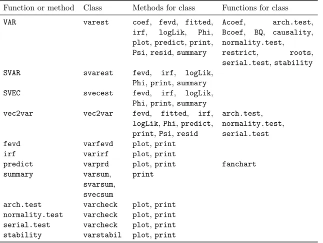
3.1. OverviewIn Table 1 the structure of the packagevars is outlined. The functions and methods will be addressed briefly here. A more detailed discussion is provided in the following subsections. When a VAR(p) has been fitted with VAR() one obtains a list object with class attribute varest.
VAR(y, p = 1, type = c("const", "trend", "both", "none"), season = NULL, exogen = NULL, lag.max = NULL,
ic = c("AIC", "HQ", "SC", "FPE"))
As one can see from Table 1, basically all relevant investigations can be conducted with the methods and functions made available for this kind of object. Plotting, prediction, forecast error variance decomposition, impulse response analysis, log-likelihood, MA representations and summary are implemented as methods. Diagnostic testing, restricted VAR estimation, stability analysis in the sense of root-stability and empirical fluctuation processes as well as causality analysis are implemented as functions. Some of the methods have their ownprint and plot methods. Furthermore, extractor methods for obtaining the residuals, the fitted values and the estimated coefficients do exist.
In Section2.2it has been argued that a VAR can be viewed as particular SVAR model. The functionSVAR() requires therefore an object of classvarest. The default estimation method of a SVAR model is a scoring algorithm, as proposed by Amisano and Giannini (1997). The restrictions for the A, B or A and B matrices have to be provided in explicit form as arguments Amat and/or Bmat. Alternatively, the different SVAR types can be estimated by directly minimizing the negative log-likelihood. The latter is used if the estimation method has then to be set toestmethod = "direct".
Function or method Class Methods for class Functions for class
VAR varest coef, fevd, fitted,
irf, logLik, Phi, plot,predict,print, Psi,resid,summary
Acoef, arch.test, Bcoef, BQ, causality, normality.test,
restrict, roots, serial.test,stability
SVAR svarest fevd, irf, logLik,
Phi,print,summary
SVEC svecest fevd, irf, logLik,
Phi,print,summary
vec2var vec2var fevd, fitted, irf,
logLik,Phi,predict, print,Psi,resid
arch.test, normality.test, serial.test
fevd varfevd plot,print
irf varirf plot,print
predict varprd plot,print fanchart
summary varsum,
svarsum, svecsum
arch.test varcheck plot,print
normality.test varcheck plot,print
serial.test varcheck plot,print
stability varstabil plot,print
Table 1: Structure of packagevars.
SVAR(x, estmethod = c("scoring", "direct"), Amat = NULL, Bmat = NULL, start = NULL, max.iter = 100, conv.crit = 1e-07, maxls = 1,
lrtest = TRUE, ...)
For objects with class attribute svarest forecast error variance decomposition, impulse re-sponse analysis, retrieval of its MA representation, the value of the log-likelihood as well as a summary are available as methods.
Structural vector error correction models can be estimated with the functionSVEC(). SVEC(x, LR = NULL, SR = NULL, r = 1, start = NULL, max.iter = 100,
conv.crit = 1e-07, maxls = 1, lrtest = TRUE, boot = FALSE, runs = 100) The returned object has class attribute svecest. The same methods that are available for objects of class svarest are at hand for these kind of objects.
Finally, objects of formal class ca.jogenerated with functionca.jo()contained in the pack-ageurcacan be converted to their level VAR representation with the functionvec2var(). The resultant object has class attribute vec2var and the analytical tools are likewise applicable as in the case of objects with class attribute varest.
3.2. Cornerstone functions
The function for estimating a VAR(p) model is VAR(). It consists of seven arguments. A data matrix or an object that can be coerced to it has to be provided fory. The lag-order has to be submitted as integer forp. In general, this lag-order is unknown and VAR() offers the possibility to automatically determine an appropriate lag inclusion. This is achieved by by setting lag.max to an upper bound integer value and ic to a desired information criteria. Possible options are Akaike (ic = "AIC"), Hannan-Quinn (ic = "HQ"), Schwarz (ic = "SC") or the forecast prediction error (ic = "FPE"). The calculations are based upon the same sample size. That is lag.max values are used for each of the estimated models as starting values.2 The type of deterministic regressors to include into the VAR(p) is set by the
argumenttype. Possible values are to include a constant, a trend, both or none deterministic regressors. In addition, the inclusion of centered seasonal dummy variables can be achieved by settingseason to the seasonal frequency of the data (e.g., for quarterly data: season = 4). Finally, exogenous variables, like intervention dummies, can be included by providing a matrix object forexogen.
Thesummary method returns – aside of descriptive information about the estimated VAR – the estimated equations as well as the variance/covariance and the correlation matrix of the residuals. It is further possible to report summary results for selected equations only. This is achieved by using the function’s argument equationwhich expects a character vector with the names of the desired endogenous variables. Theplot method displays for each equation in a VAR a diagram of fit, a residual plot, the auto-correlation and partial auto-correlation function of the residuals in a single layout. If the plot method is called interactively, the user is requested to enter <RETURN> for commencing to the next plot. It is further possible to plot the results for a subset of endogenous variables only. This is achieved by using the argument name in the plot method. The appearance of the plot can be adjusted to ones liking by setting the relevant arguments of theplot method.
A SVAR model is estimated with the functionSVAR(). An object with class attributevarest has to be provided as argument for x. The structural parameters are estimated either by a scoring algorithm (the default) or by direct minimization of the negative log-likelihood function. Whether an A,B orAB model will be estimated, is dependent on the setting for Amatand Bmat. If a restriction matrix forAmat with dimension (K×K) is provided and the argumentBmatis leftNULL, anA model will be estimated. In this caseBmat is set internally to an identity matrix IK. Alternatively, if only a matrix object for Bmat is provided and Amat is left unchanged, then a B model will be estimated and internally Amat is set to an identity matrix IK. Finally, if matrix objects for both arguments are provided, then an AB model will be estimated. In all cases, the matrix elements to be estimated are marked byNA entries at the relevant positions. The user has the option to provide starting values for the unknown coefficients by providing a vector object for the argument start. If start is left NULL, then0.1will be used as the starting value for all coefficients. The argumentsmax.iter, conv.critand maxls can be used for tuning the scoring algorithm. The maximum number of iterations is controlled bymax.iter, the convergence criterion is set byconv.critand the maximum step length is set bymaxls. A likelihood ratio test is computed per default for
over-2
As an alternative one can use the functionVARselect(). The result of this function is a list object with elementsselectionandcriteria. The elementselectionis a vector of optimal lag length according to the above mentioned information criteria. The elementcriteria is a matrix containing the particular values for each of these criteria up to the maximal chosen lag order.
identified systems. This default setting can be offset bylrtest = FALSE. If a just-identified has been set-up, a warning is issued that an over-identification test cannot be computed in case of lrtest = TRUE. The ellipsis argument (...) is passed to optim() in case of direct optimization.
The returned object of function SVAR() is a list with class attribute svarest. Depen-dent on the chosen model and if the argument hessian = TRUE has been set in case of estmethod = "direct", the list elements A, Ase, B, Bsecontain the estimated coefficient matrices with the numerical standard errors. The element LRIM does contain the long-run impact matrix in case a SVAR of type Blanchard & Quah is estimated with function BQ(), otherwise this element is NULL (see Blanchard and Quah 1989). The list element Sigma.U is the variance-covariance matrix of the reduced form residuals times 100, i.e., ΣU = A−1BB>A−1
>
×100. The list element LR is an object with class attribute htest, holding the likelihood ratio over-identification test. The element opt is the returned object from functionoptim()in caseestmethod = "direct"has been used. The remaining five list items are the vector of starting values, the SVAR model type, thevarest object, the number of iterations and thecall toSVAR().
A SVEC model is estimated with the functionSVEC(). The supplied object for the argument xmust be of formal class ca.jo. The restrictions on the long-run and short-run structural coefficient matrices must be provided as arguments LR and SR, respectively. These matrices have either zero orNA entries as their elements. It is further necessary to specify the cointe-gration rank of the estimated VECM via the argumentr. Likewise toSVAR(), the arguments start, max.iter,conv.crit and maxls can be used for tuning the scoring algorithm. The argument lrtest applies likewise as in SVAR(). Finally, the logical flag boot can be used for calculating standard errors by applying the bootstrap method to the SVEC. The count of repetition is set by the argument runs. The returned list object from SVEC() and its associated methods will be bespoken in Section4, where a SVEC model is specified for the Canadian labor market.
Finally, with function vec2var() a VECM (i.e., an object of formal class ca.jo, generated by the function ca.jo() contained in the package urca) is transformed into its level-VAR representation. Aside of this argument the function requires the cointegrating rank as this information is needed for the transformation (see Equations 12–16). The print method does return the coefficient values, first for the lagged endogenous variables, next for the deterministic regressors.
3.3. Diagnostic testing
In the package vars functions for diagnostic testing are arch.test(), normality.test(), serial.test()and stability(). The former three functions return a list object with class attributevarcheckfor whichplotandprintmethod exist. The plots – one for each equation – include a residual plot, an empirical distribution plot and the ACF and PACF of the residuals and their squares. Theplotmethod offers additional arguments for adjusting its appearance. The implemented tests for heteroscedasticity are the univariate and multivariate ARCH test (seeEngle 1982;Hamilton 1994;L¨utkepohl 2006). The multivariate ARCH-LM test is based on the following regression (the univariate test can be considered as special case of the exhi-bition below and is skipped):
whereby vt assigns a spherical error process and vech is the column-stacking operator for symmetric matrices that stacks the columns from the main diagonal on downward. The dimension ofβ0 is 12K(K+ 1) and for the coefficient matricesBi withi= 1, . . . , q, 12K(K+ 1)×1
2K(K+ 1). The null hypothesis is: H0 :=B1 =B2 =. . .=Bq= 0 and the alternative is: H1 :B1 6= 0∩B26= 0∩. . .∩Bq6= 0. The test statistic is defined as:
VARCHLM(q) = 1 2T K(K+ 1)R 2 m , (21) with R2m = 1− 2 K(K+ 1)tr( ˆΩ ˆΩ −1 0 ) , (22)
and ˆΩ assigns the covariance matrix of the above defined regression model. This test statistic is distributed asχ2(qK2(K+ 1)2/4).
The default is to compute the multivariate test only. If multivariate.only = FALSE, the univariate tests are computed too. In this case, the returned list object from arch.test() has three elements. The first element is the matrix of residuals. The second, signified by arch.uni, is a list object itself and holds the univariate test results for each of the series. The multivariate test result is contained in the third list element, signified byarch.mul.
arch.test(x, lags.single = 16, lags.multi = 5, multivariate.only = TRUE) The returned tests have class attribute htest, hence the print method for these kind of objects is implicitly used asprintmethod for objects of classvarcheck. This applies likewise to the functionsnormality.test() and serial.test(), which will be bespoken next. The Jarque-Bera normality tests for univariate and multivariate series are implemented and applied to the residuals of a VAR(p) as well as separate tests for multivariate skewness and kurtosis (see Bera and Jarque 1980, 1981; Jarque and Bera 1987; L¨utkepohl 2006). The univariate versions of the Jarque-Bera test are applied to the residuals of each equation. A multivariate version of this test can be computed by using the residuals that are standardized by a Choleski decomposition of the variance-covariance matrix for the centered residuals. Please note, that in this case the test result is dependent upon the ordering of the variables. The test statistics for the multivariate case are defined as:
J Bmv =s23+s24 , (23) whereby s23 and s24 are computed according to:
s23 =Tb>1b1/6 (24a)
s24 =T(b2−3K)>(b2−3k)/24, (24b) with b1 and b2 are the third and fourth non-central moment vectors of the standardized residuals ˆust = ˜P−(ˆut−u¯ˆt) and ˜P is a lower triangular matrix with positive diagonal such that ˜PP˜>= ˜Σu, i.e., the Choleski decomposition of the residual covariance matrix. The test
statistic J Bmv is distributed as χ2(2K) and the multivariate skewness,s23, and kurtosis test,
s24 are distributed asχ2(K).
The matrix of residuals is the first element in the returned list object. The function’s default is to compute the multivariate test statistics only. The univariate tests are re-turned ifmultivariate.only = FALSE is set. Similar to the returned list object of function arch.test()for this case, the univariate versions of the Jarque-Bera test are applied to the residuals of each equation and are contained in the second list element signified by jb.uni. The multivariate version of the test as well as multivariate tests for skewness and kurtosis are contained in the third list element signified byjb.mul.
For testing the lack of serial correlation in the residuals of a VAR(p), a Portmanteau test and the Breusch-Godfrey LM test are implemented in the functionserial.test(). For both tests small sample modifications can be calculated too, whereby the modification for the LM test has been introduced byEdgerton and Shukur(1999).
The Portmanteau statistic is defined as:
Qh=T h
X
j=1
tr( ˆCj>Cˆ0−1CˆjCˆ0−1), (25)
with ˆCi= T1ΣTt=i+1uˆtuˆ>t−i. The test statistic has an approximate χ2(K2h−n∗) distribution, andn∗ is the number of coefficients excluding deterministic terms of a VAR(p). The limiting distribution is only valid for h tending to infinity at a suitable rate with growing sample size. Hence, the trade-off is between a decent approximation to theχ2 distribution and a loss in power of the test, when h is chosen too large. The small sample adjustment of the test statistic is given as:
Q∗h=T2 h X j=1 1 T −jtr( ˆC > j Cˆ0−1CˆjCˆ0−1), (26)
and is computed if type = "PT.adjusted"is set.
The Breusch-Godfrey LM statistic is based upon the following auxiliary regressions (see
Breusch 1978;Godfrey 1978): ˆ
ut=A1yt−1+. . .+Apyt−p+CDt+B1uˆt−1+. . .+Bhuˆt−h+εt. (27) The null hypothesis is: H0 :B1 =· · ·=Bh = 0 and correspondingly the alternative hypothesis is of the form H1 :∃Bi 6= 0f or i= 1,2, . . . , h. The test statistic is defined as:
LMh =T(K−tr( ˜Σ−R1Σ˜e)) , (28) where ˜ΣR and ˜Σe assign the residual covariance matrix of the restricted and unrestricted model, respectively. The test statisticLMh is distributed as χ2(hK2). Edgerton and Shukur (1999) proposed a small sample correction, which is defined as:
LMFh= 1−(1−Rr2)1/r (1−R2 r)1/r N r−q Km , (29) with R2r = 1− |Σ˜e|/|Σ˜R|, r = ((K2m2−4)/(K2+m2−5))1/2, q = 1/2Km−1 and N =
T−K−m−1/2(K−m+ 1), whereby nis the number of regressors in the original system and m = Kh. The modified test statistic is distributed as F(hK2, int(N r−q)). This test statistic is returned iftype = "ES" has been used.
serial.test(x, lags.pt = 16, lags.bg = 5,
type = c("PT.asymptotic", "PT.adjusted", "BG", "ES"))
The test statistics are returned in the list element serial and have class attribute htest. Per default the asymptotic Portmanteau test is returned. The residuals are contained in the first list element.
The functionstability()returns a list object with class attributevarstabil. The function itself is just a wrapper for the functionefp()contained in the packagestrucchange(seeZeileis, Leisch, Hornik, and Kleiber 2002, for a detailed exposition of the package’s capabilities). The first element of the returned list object is itself a list of objects with class attribute efp. Hence, theplotmethod for objects of classvarstabiljust calls theplotmethod for objects of classefp.
stability(x, type = c("OLS-CUSUM", "Rec-CUSUM", "Rec-MOSUM",
"OLS-MOSUM", "RE", "ME", "Score-CUSUM", "Score-MOSUM", "fluctuation"), h = 0.15, dynamic = FALSE, rescale = TRUE)
3.4. Evaluating model forecasts
A predict method for objects with class attribute varest or vec2var is available. The n.aheadforecasts are computed recursively for the estimated VAR(p)-process and a value for the forecast confidence interval can be provided too. Its default value is0.95. The confidence interval is inferred from the empirical forecast error covariance matrix.
predict(object, ..., n.ahead = 10, ci = 0.95, dumvar = NULL)
Thepredict method returns a list with class attributevarprd. The forecasts are contained as a list in its first element signified as fcst. The second entry are the endogenous vari-ables themselves. The last element is the submitted model object to predict. The print method returns the forecasts with upper and lower confidence levels, if applicable. Theplot method draws the time series plots, whereby the start of the out-of-sample period is marked by a dashed vertical line. If this method is called interactively, the user is requested to browse through the graphs for each variable by hitting the <RETURN> key. For visualizing forecasts (i.e., objects with class attributevarprd) fan charts can be generated by the func-tionfanchart() (see Britton, Fisher, and Whitley 1998). If the functional argument color is not set, the colors are taken from the gray color scheme. Likewise, if no confidence levels are supplied, then the fan charts are produced for confidence levels ranging from0.1to0.9 with step size0.1.
fanchart(x, colors = NULL, cis = NULL, names = NULL, main = NULL,
ylab = NULL, xlab = NULL, col.y = NULL, nc, plot.type = c("multiple", "single"), mar = par("mar"), oma = par("oma"), ...)
The impulse response analysis is based upon the Wold moving average representation of a VAR(p)-process (see Equations 5 and 6 above). It is used to investigate the dynamic interactions between the endogenous variables. The (i, j)thcoefficients of the matrices Φsare thereby interpreted as the expected response of variable yi,t+s to a unit change in variable
yjt. These effects can be accumulated through time,s= 1,2, . . ., and hence one would obtain the simulated impact of a unit change in variablej to the variableiat times. Aside of these impulse response coefficients, it is often conceivable to use orthogonal impulse responses as an alternative. This is the case, if the underlying shocks are less likely to occur in isolation, but when contemporaneous correlations between the components of the error processutexist, i.e., the off-diagonal elements of Σu are non-zero. The orthogonal impulse responses are derived
from a Choleski decomposition of the error variance-covariance matrix: Σu = P P> with P
being a lower triangular. The moving average representation can then be transformed to:
yt= Ψ0εt+ Ψ1εt−1+. . . , (30) with εt = P−1ut and Ψi = ΦiP for i = 0,1,2, . . . and Ψ0 = P. Incidentally, because the matrixP is lower triangular, it follows that only a shock in the first variable of a VAR(p )-process does exert an influence on all the remaining ones and that the second and following variables cannot have a direct impact on y1t. Please note, that a different ordering of the variables might produce different outcomes with respect to the impulse responses. The non-uniqueness of the impulse responses can be circumvented by analyzing a set of endogenous variables in the SVAR framework.
Impulse response analysis has been implemented as a method for objects with class attribute of either varest, svarest, svecest or vec2var. These methods are utilizing the methods PhiandPsi, where applicable.
irf(x, impulse = NULL, response = NULL, n.ahead = 10, ortho = TRUE,
cumulative = FALSE, boot = TRUE, ci = 0.95, runs = 100, seed = NULL, ...) The impulse variables are set as a character vector impulse and the responses are provided likewise in the argumentresponse. If either one is unset, then all variables are considered as impulses or responses, respectively. The default length of the impulse responses is set to 10 via argument n.ahead. The computation of orthogonal and/or cumulative impulse responses is controlled by the logical switchesortho and cumulative, respectively. Finally, confidence bands can be returned by setting boot = TRUE (default). The preset values are to run 100 replications and return 95% confidence bands. It is at the user’s leisure to specify a seed for the random number generator. The standard percentile interval is calculated as
CIs = [s∗γ/2, s∗(1−γ)/2], where sγ/2∗ and s∗(1−γ)/2 are the γ/2 and (1−γ)/2 quantiles of the estimated bootstrapped impulse response coefficients ˆΦ∗ or ˆΨ∗ (see Efron and Tibshirani 1993). Theirfmethod returns a list object with class attributevarirffor whichprintand plotmethods do exist. Likewise to the plotmethod of objects with class attribute varprd, the user is requested to browse through the graphs for each variable by hitting the<RETURN> key, whence the method is called interactively. The appearance of the plots can be adjusted. The forecast error variance decomposition is based upon the orthogonal impulse response coefficient matrices Ψn. The FEVD allows the user to analyze the contribution of variablejto theh-step forecast error variance of variablek. If the element-wise squared orthogonal impulse responses are divided by the variance of the forecast error variance,σk2(h), the resultant is a percentage figure. Thefevd method is available for conducting FEVD. Methods for objects of classes varest, svarest, svecest and vec2var do exist. Aside of the object itself, the argumentn.aheadcan be specified; its default value is10.
The method returns a list object with class attribute varfevd for which print and plot methods do exist. The list elements are the forecast error variances organized on a per-variable basis. Theplotmethod for these objects is similar to the ones for objects with class attributevarirfand/or varprd and the appearance of the plots can be adjusted too.
4. Example
Functions and methods from the last section are now illustrated with a macro economic data set for Canada. It is shown how the results presented in Breitung, Br¨uggemann, and L¨utkepohl (2004) can be replicated. However, theR code snippets should illustrate the ease of application rather than commenting and interpreting the results in depth.
The authors investigated the Canadian labor market. They utilized the following series: labor productivity defined as the log difference between GDP and employment, the log of employment, the unemployment rate and real wages, defined as the log of the real wage index. These series are signified by “prod”, “e”, “U” and “rw”, respectively. The data is taken from the OECD data base and spans from the first quarter 1980 until the fourth quarter 2004. In a first step the packagevarsis loaded into the workspace. The Canadian data set which is included in the packagevars is brought into memory.
R> library("vars") R> data("Canada") R> summary(Canada)
e prod rw U
Min. :929 Min. :401 Min. :386 Min. : 6.70
1st Qu.:935 1st Qu.:405 1st Qu.:424 1st Qu.: 7.78 Median :946 Median :406 Median :444 Median : 9.45
Mean :944 Mean :408 Mean :441 Mean : 9.32
3rd Qu.:950 3rd Qu.:411 3rd Qu.:461 3rd Qu.:10.61
Max. :962 Max. :418 Max. :470 Max. :12.77
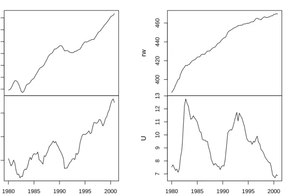
R> plot(Canada, nc = 2, xlab = "")
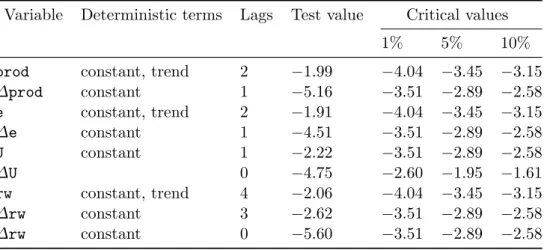
A preliminary data analysis is conducted by displaying the summary statistics of the series involved as well as the corresponding time series plots (see Figure1). In a next step, the authors conducted unit root tests by applying the Augmented Dickey-Fuller test regressions to the series (henceforth: ADF test). The ADF test has been implemented in the packageurca as functionur.df(), for instance. The result of the ADF tests are summarized in Table2.3 R> adf1 <- summary(ur.df(Canada[, "prod"], type = "trend", lags = 2))
R> adf1
############################################### # Augmented Dickey-Fuller Test Unit Root Test #
3
In the following onlyRcode excerpts are shown. TheRcode for producing the Tables and Figures below are provided in a separate file that accompanies this text.
930 940 950 960 e 405 410 415 1980 1985 1990 1995 2000 prod 400 420 440 460 rw 7 8 9 10 11 12 13 1980 1985 1990 1995 2000 U Canada
Figure 1: Canadian labor market time series.
############################################### Test regression trend
Call:
lm(formula = z.diff ~ z.lag.1 + 1 + tt + z.diff.lag) Residuals:
Min 1Q Median 3Q Max
-2.1992 -0.3899 0.0429 0.4191 1.7166 Coefficients:
Estimate Std. Error t value Pr(>|t|) (Intercept) 30.41523 15.30940 1.99 0.051 .
z.lag.1 -0.07579 0.03813 -1.99 0.050 .
tt 0.01390 0.00642 2.16 0.034 *
z.diff.lag1 0.28487 0.11436 2.49 0.015 *
---Signif. codes: 0 '***' 0.001 '**' 0.01 '*' 0.05 '.' 0.1 ' ' 1 Residual standard error: 0.685 on 76 degrees of freedom
Multiple R-squared: 0.135, Adjusted R-squared: 0.0899 F-statistic: 2.98 on 4 and 76 DF, p-value: 0.0244
Value of test-statistic is: -1.9875 2.3 2.3817 Critical values for test statistics:
1pct 5pct 10pct tau3 -4.04 -3.45 -3.15 phi2 6.50 4.88 4.16 phi3 8.73 6.49 5.47
R> adf2 <- summary(ur.df(diff(Canada[, "prod"]), type = "drift", + lags = 1))
R> adf2
############################################### # Augmented Dickey-Fuller Test Unit Root Test # ############################################### Test regression drift
Call:
lm(formula = z.diff ~ z.lag.1 + 1 + z.diff.lag) Residuals:
Min 1Q Median 3Q Max
-2.0512 -0.3953 0.0782 0.4111 1.7513 Coefficients:
Estimate Std. Error t value Pr(>|t|)
(Intercept) 0.1153 0.0803 1.44 0.15
z.lag.1 -0.6889 0.1335 -5.16 1.8e-06 ***
z.diff.lag -0.0427 0.1127 -0.38 0.71
---Signif. codes: 0 '***' 0.001 '**' 0.01 '*' 0.05 '.' 0.1 ' ' 1 Residual standard error: 0.697 on 78 degrees of freedom
Multiple R-squared: 0.361, Adjusted R-squared: 0.345 F-statistic: 22.1 on 2 and 78 DF, p-value: 2.53e-08
Variable Deterministic terms Lags Test value Critical values
1% 5% 10%
prod constant, trend 2 −1.99 −4.04 −3.45 −3.15
∆prod constant 1 −5.16 −3.51 −2.89 −2.58 e constant, trend 2 −1.91 −4.04 −3.45 −3.15 ∆e constant 1 −4.51 −3.51 −2.89 −2.58 U constant 1 −2.22 −3.51 −2.89 −2.58 ∆U 0 −4.75 −2.60 −1.95 −1.61 rw constant, trend 4 −2.06 −4.04 −3.45 −3.15 ∆rw constant 3 −2.62 −3.51 −2.89 −2.58 ∆rw constant 0 −5.60 −3.51 −2.89 −2.58
Table 2: ADF tests for Canadian data.
Value of test-statistic is: -5.1604 13.318 Critical values for test statistics:
1pct 5pct 10pct tau2 -3.51 -2.89 -2.58 phi1 6.70 4.71 3.86
It can be concluded that all time series are integrated of order one. Please note, that the reported critical values differ slightly from the ones that are reported inBreitunget al.(2004). The authors utilized the softwareJMulTi (L¨utkepohl and Kr¨atzig 2004) in which the critical values of Davidson and MacKinnon (1993) are used, whereas in the function ur.df() the critical values are taken from Dickey and Fuller (1981) and Hamilton(1994).
In an ensuing step, the authors determined an optimal lag length for an unrestricted VAR for a maximal lag length of eight.
R> VARselect(Canada, lag.max = 8, type = "both")
$selection AIC(n) HQ(n) SC(n) FPE(n) 3 2 1 3 $criteria 1 2 3 4 5 6 AIC(n) -6.2725791 -6.6366697 -6.7711769 -6.6346092 -6.3981322 -6.3077048 HQ(n) -5.9784294 -6.1464203 -6.0848278 -5.7521604 -5.3195837 -5.0330565 SC(n) -5.5365580 -5.4099679 -5.0537944 -4.4265460 -3.6993884 -3.1182803 FPE(n) 0.0018898 0.0013195 0.0011660 0.0013632 0.0017821 0.0020442 7 8 AIC(n) -6.0707273 -6.0615969 HQ(n) -4.5999792 -4.3947490
SC(n) -2.3906220 -1.8908109 FPE(n) 0.0027686 0.0030601
According to the AIC and FPE the optimal lag number is p = 3, whereas the HQ criterion indicatesp= 2 and the SC criterion indicates an optimal lag length ofp= 1. They estimated for all three lag orders a VAR including a constant and a trend as deterministic regressors and conducted diagnostic tests with respect to the residuals. In theR code example below, the relevant commands are exhibited for the VAR(1) model. First, the variables have to be reordered in the same sequence as in Breitung et al. (2004). This step is necessary, because otherwise the results of the multivariate Jarque-Bera test, in which a Choleski decomposition is employed, would differ slightly from the reported ones in Breitung et al. (2004). In the R code lines below the estimation of the VAR(1) as well as the summary output and the diagram of fit for equation “e” is shown.
R> Canada <- Canada[, c("prod", "e", "U", "rw")] R> p1ct <- VAR(Canada, p = 1, type = "both") R> p1ct
VAR Estimation Results: =======================
Estimated coefficients for equation prod: ========================================= Call:
prod = prod.l1 + e.l1 + U.l1 + rw.l1 + const + trend
prod.l1 e.l1 U.l1 rw.l1 const trend
0.963137 0.012912 0.211089 -0.039094 16.243407 0.046131
Estimated coefficients for equation e: ====================================== Call:
e = prod.l1 + e.l1 + U.l1 + rw.l1 + const + trend
prod.l1 e.l1 U.l1 rw.l1 const trend
0.194650 1.238923 0.623015 -0.067763 -278.761211 -0.040660
Estimated coefficients for equation U: ====================================== Call:
U = prod.l1 + e.l1 + U.l1 + rw.l1 + const + trend
prod.l1 e.l1 U.l1 rw.l1 const trend
Estimated coefficients for equation rw: ======================================= Call:
rw = prod.l1 + e.l1 + U.l1 + rw.l1 + const + trend
prod.l1 e.l1 U.l1 rw.l1 const trend
-0.223087 -0.051044 -0.368640 0.948909 163.024531 0.071422 R> summary(p1ct, equation = "e")
VAR Estimation Results: =========================
Endogenous variables: prod, e, U, rw Deterministic variables: both
Sample size: 83
Log Likelihood: -207.525
Roots of the characteristic polynomial: 0.95 0.95 0.904 0.751
Call:
VAR(y = Canada, p = 1, type = "both")
Estimation results for equation e: ==================================
e = prod.l1 + e.l1 + U.l1 + rw.l1 + const + trend Estimate Std. Error t value Pr(>|t|)
prod.l1 0.1947 0.0361 5.39 7.5e-07 *** e.l1 1.2389 0.0863 14.35 < 2e-16 *** U.l1 0.6230 0.1693 3.68 0.00043 *** rw.l1 -0.0678 0.0283 -2.40 0.01899 * const -278.7612 75.1830 -3.71 0.00039 *** trend -0.0407 0.0197 -2.06 0.04238 * ---Signif. codes: 0 '***' 0.001 '**' 0.01 '*' 0.05 '.' 0.1 ' ' 1
Residual standard error: 0.47 on 77 degrees of freedom
Multiple R-Squared: 1, Adjusted R-squared: 1
F-statistic: 5.58e+07 on 6 and 77 DF, p-value: <2e-16
Covariance matrix of residuals:
prod e U rw
e 0.06767 0.2210 -0.1320 -0.08279 U -0.04128 -0.1320 0.1216 0.06374 rw 0.00214 -0.0828 0.0637 0.59317 Correlation matrix of residuals:
prod e U rw
prod 1.00000 0.210 -0.173 0.00406 e 0.21008 1.000 -0.805 -0.22869 U -0.17275 -0.805 1.000 0.23731 rw 0.00406 -0.229 0.237 1.00000 R> plot(p1ct, names = "e")
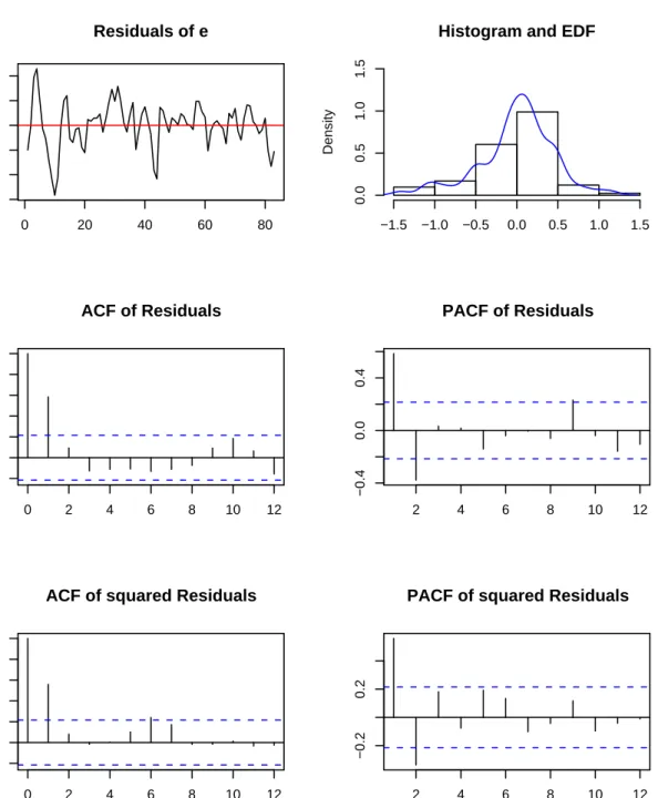
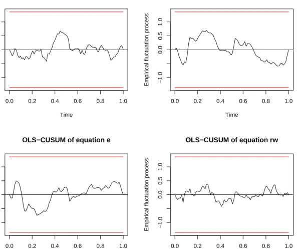
The resulting graphic is displayed in Figure2. Next, it is shown how the diagnostic tests are conducted for the VAR(1) model. The results of all diagnostic tests, i.e., for the VAR(1), VAR(2) and VAR(3) model, are provided in Table3 and the graphics of thevarcheckobject arch1 for the employment equation and the OLS-CUSUM tests for the VAR(1) model are shown in Figures 3 and 4, respectively.
R> ser11 <- serial.test(p1ct, lags.pt = 16, type = "PT.asymptotic") R> ser11$serial
Portmanteau Test (asymptotic) data: Residuals of VAR object p1ct
Chi-squared = 233.5, df = 240, p-value = 0.606 R> norm1 <- normality.test(p1ct)
R> norm1$jb.mul $JB
JB-Test (multivariate) data: Residuals of VAR object p1ct
Chi-squared = 9.9189, df = 8, p-value = 0.2708
$Skewness
Skewness only (multivariate) data: Residuals of VAR object p1ct
Chi-squared = 6.356, df = 4, p-value = 0.1741
405
410
415
Diagram of fit and residuals for e
0 20 40 60 80 −2 −1 0 1 0 2 4 6 8 10 12 −0.2 0.6 Lag ACF Residuals 2 4 6 8 10 12 −0.2 0.1 Lag PACF Residuals
Figure 2: Plot of VAR(1) for equation “e”.
Model Q16 pvalue Q∗16 p value JB4 pvalue MARCH5 p value
p= 3 174.0 0.96 198.0 0.68 9.66 0.29 512.0 0.35
p= 2 209.7 0.74 236.1 0.28 2.29 0.97 528.1 0.19
p= 1 233.5 0.61 256.9 0.22 9.92 0.27 570.1 0.02
Residuals of e 0 20 40 60 80 −1.5 −0.5 0.5 0 2 4 6 8 10 12 −0.2 0.2 0.6 1.0 ACF of Residuals 0 2 4 6 8 10 12 −0.2 0.2 0.6 1.0
ACF of squared Residuals
Histogram and EDF
Density −1.5 −1.0 −0.5 0.0 0.5 1.0 1.5 0.0 0.5 1.0 1.5 2 4 6 8 10 12 −0.4 0.0 0.4 PACF of Residuals 2 4 6 8 10 12 −0.2 0.2
PACF of squared Residuals
OLS−CUSUM of equation prod
Time
Empirical fluctuation process
0.0 0.2 0.4 0.6 0.8 1.0 −1.0 0.0 0.5 1.0 OLS−CUSUM of equation e Time
Empirical fluctuation process
0.0 0.2 0.4 0.6 0.8 1.0 −1.0 0.0 0.5 1.0 OLS−CUSUM of equation U Time
Empirical fluctuation process
0.0 0.2 0.4 0.6 0.8 1.0 −1.0 0.0 0.5 1.0 OLS−CUSUM of equation rw Time
Empirical fluctuation process
0.0 0.2 0.4 0.6 0.8 1.0
−1.0
0.0
0.5
1.0
Figure 4: OLS-CUSUM test of VAR(1).
Kurtosis only (multivariate) data: Residuals of VAR object p1ct
Chi-squared = 3.5629, df = 4, p-value = 0.4684 R> arch1 <- arch.test(p1ct, lags.multi = 5) R> arch1$arch.mul
ARCH (multivariate)
data: Residuals of VAR object p1ct
Chi-squared = 570.14, df = 500, p-value = 0.01606 R> plot(arch1, names = "e")
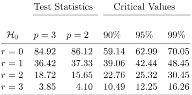
Test Statistics Critical Values H0 p= 3 p= 2 90% 95% 99% r= 0 84.92 86.12 59.14 62.99 70.05 r= 1 36.42 37.33 39.06 42.44 48.45 r= 2 18.72 15.65 22.76 25.32 30.45 r= 3 3.85 4.10 10.49 12.25 16.26
Table 4: Johansen cointegration tests for Canadian system.
Given the diagnostic test results the authors concluded that a VAR(1)-specification might be too restrictive. They argued further, that although some of the stability tests do indicate deviations from parameter constancy, the time-invariant specification of the VAR(2) and VAR(3) model will be maintained as tentative candidates for the following cointegration analysis.
The authors estimated a VECM whereby a deterministic trend has been included in the cointegration relation. The estimation of these models as well as the statistical inference with respect to the cointegration rank can be swiftly accomplished with the function ca.jo(). Although the following R code examples are using functions contained in the package urca, it is however beneficial to reproduce these results for two reasons: the interplay between the functions contained in package urca and vars is exhibited and it provides an understanding of the then following SVEC specification.
R> summary(ca.jo(Canada, type = "trace", ecdet = "trend", K = 3, + spec = "transitory"))
R> summary(ca.jo(Canada, type = "trace", ecdet = "trend", K = 2, + spec = "transitory"))
The outcome of the trace tests is provided in Table4. These results do indicate one cointegra-tion relacointegra-tionship. The reported critical values differ slightly from the ones that are reported in Table 4.3 of Breitung et al. (2004). The authors used the values that are contained in
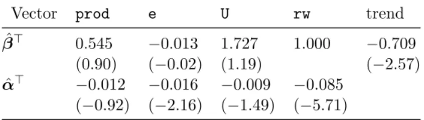
Johansen (1995), whereas the values from Osterwald-Lenum(1992) are used in the function ca.jo(). In the Rcode snippet below the VECM is re-estimated with this restriction and a normalization of the long-run relationship with respect to real wages. The results are shown in Table 5.
R> vecm <- ca.jo(Canada[, c("rw", "prod", "e", "U")], type = "trace", + ecdet = "trend", K = 3, spec = "transitory")
R> vecm.r1 <- cajorls(vecm, r = 1)
For a just identified SVEC model of type B one needs 12K(K−1) = 6 linear independent restrictions. It is further reasoned from the Beveridge-Nelson decomposition that there are
k∗=r(K−r) = 3 shocks with permanent effects and only one shock that exerts a temporary effect, due to r = 1. Because the cointegration relation is interpreted as a stationary wage-setting relation, the temporary shock is associated with the wage shock variable. Hence, the
Vector prod e U rw trend ˆ β> 0.545 −0.013 1.727 1.000 −0.709 (0.90) (−0.02) (1.19) (−2.57) ˆ α> −0.012 −0.016 −0.009 −0.085 (−0.92) (−2.16) (−1.49) (−5.71)
Table 5: Cointegration vector and loading parameters (witht statistics in parentheses).
four entries in the last column of the long-run impact matrix ΞB are set to zero. Because this matrix is of reduced rank, only k∗r = 3 linear independent restrictions are imposed thereby. It is therefore necessary to set 12k∗(k∗ −1) = 3 additional elements to zero. The authors assumed constant returns of scale and therefore productivity is only driven by output shocks. This reasoning implies zero coefficients in the first row of the long-run matrix for the variables employment, unemployment and real wages, hence the elements ΞB1,j forj = 2,3,4 are set to zero. Because ΞB1,4 has already been set to zero, only two additional restrictions have been added. The last restriction is imposed on the element B4,2. Here, it is assumed that labor demand shocks do not exert an immediate effect on real wages.
In the R code example below the matrix objects LR and SR are set up accordingly and the just-identified SVEC is estimated with functionSVEC(). In the call to the functionSVEC()the argumentboot = TRUEhas been employed such that bootstrapped standard errors and hence
t statistics can be computed for the structural long-run and contemporaneous coefficients. R> vecm <- ca.jo(Canada[, c("prod", "e", "U", "rw")], type = "trace",
+ ecdet = "trend", K = 3, spec = "transitory") R> SR <- matrix(NA, nrow = 4, ncol = 4)
R> SR[4, 2] <- 0
R> LR <- matrix(NA, nrow = 4, ncol = 4) R> LR[1, 2:4] <- 0
R> LR[2:4, 4] <- 0
R> svec <- SVEC(vecm, LR = LR, SR = SR, r = 1, lrtest = FALSE, boot = TRUE, + runs = 100)
R> summary(svec)
SVEC Estimation Results: ======================== Call:
SVEC(x = vecm, LR = LR, SR = SR, r = 1, lrtest = FALSE, boot = TRUE, runs = 100)
Type: B-model Sample size: 81
Log Likelihood: -161.838 Number of iterations: 10
Estimated contemporaneous impact matrix: prod e U rw prod 0.5840 0.0743 -0.15258 0.0690 e -0.1203 0.2614 -0.15510 0.0898 U 0.0253 -0.2672 0.00549 0.0498 rw 0.1117 0.0000 0.48377 0.4879
Estimated standard errors for impact matrix:
prod e U rw
prod 0.0803 0.1047 0.2125 0.0660 e 0.0705 0.0596 0.1665 0.0402 U 0.0527 0.0433 0.0568 0.0309 rw 0.1462 0.0000 0.6142 0.0888 Estimated long run impact matrix:
prod e U rw
prod 0.791 0.000 0.000 0
e 0.202 0.577 -0.492 0
U -0.159 -0.341 0.141 0 rw -0.153 0.596 -0.250 0
Estimated standard errors for long-run matrix:
prod e U rw
prod 0.152 0.0000 0.000 0 e 0.230 0.1801 0.550 0 U 0.115 0.0884 0.149 0 rw 0.184 0.1549 0.264 0
Covariance matrix of reduced form residuals (*100):
prod e U rw
prod 37.464 -2.10 -0.251 2.51 e -2.096 11.49 -6.927 -4.47 U -0.251 -6.93 7.454 2.98 rw 2.509 -4.47 2.978 48.46
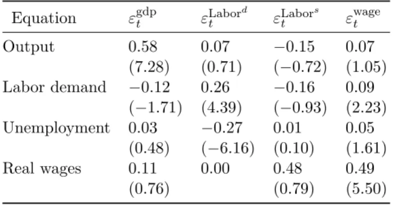
The results are summarized in the Tables6and7. The values of thetstatistics differ slightly from the reported ones inBreitunget al. (2004) which can be attributed to sampling. In the Rcode example above only 100 runs have been executed, whereas in Breitung et al. (2004) 2000 repetitions have been used.
The authors investigated further if labor supply shocks do have no long-run impact on unem-ployment. This hypothesis is mirrored by setting ΞB3,3 = 0. Because one more zero restriction has been added to the long-run impact matrix, the SVEC model is now over-identified. The validity of this over-identification restriction can be tested with a LR test. In the R code example below first the additional restriction has been set and then the SVEC is re-estimated by using the upate method. The result of the LR test is contained in the returned list as named element LRover.
Equation εgdpt εLabort d εLabort s εwaget Output 0.58 0.07 −0.15 0.07 (7.28) (0.71) (−0.72) (1.05) Labor demand −0.12 0.26 −0.16 0.09 (−1.71) (4.39) (−0.93) (2.23) Unemployment 0.03 −0.27 0.01 0.05 (0.48) (−6.16) (0.10) (1.61) Real wages 0.11 0.00 0.48 0.49 (0.76) (0.79) (5.50)
Table 6: Estimated coefficients of the contemporaneous impact matrix (with t statistics in parentheses).
Equation εgdpt εLabort d εLabort s εwaget
Output 0.79 0.00 0.00 0.00 (5.21) Labor demand 0.20 0.58 −0.49 0.00 (0.88) (3.20) (−0.89) Unemployment −0.16 −0.34 0.14 0.00 (−1.38) (−3.86) (0.95) Real wages −0.15 0.60 −0.25 0.00 (−0.83) (3.85) (−0.95)
Table 7: Estimated coefficients of the long-run impact matrix (withtstatistics in parentheses).
R> LR[3, 3] <- 0
R> svec.oi <- update(svec, LR = LR, lrtest = TRUE, boot = FALSE) R> svec.oi$LRover
LR overidentification data: vecm
Chi^2 = 6.0745, df = 1, p-value = 0.01371
The value of the test statistic is 6.07 and thepvalue of thisχ2(1)-distributed variable is 0.014. Therefore, the null hypothesis that shocks to the labor supply do not exert a long-run effect on unemployment has to be rejected for a significance level of 5%.
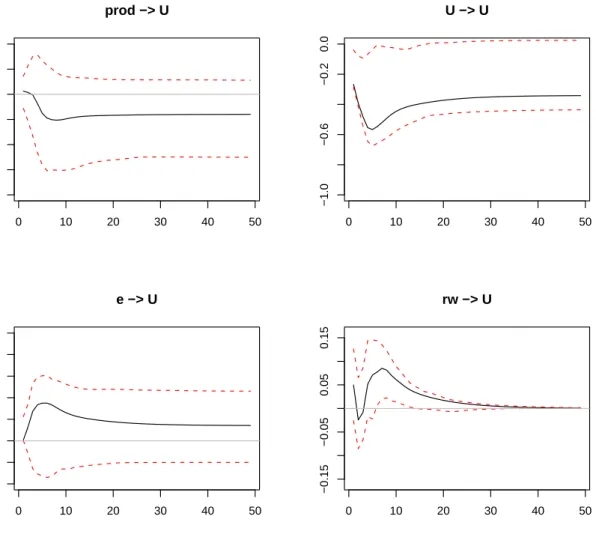
In order to investigate the dynamic effects on unemployment, the authors applied an impulse response analysis. The impulse response analysis shows the effects of the different shocks, i.e., output, labor demand, labor supply and wage, to unemployment. In theRcode example below theirfmethod for objects with class attributesvecestis employed and the argument boot = TRUEhas been set such that confidence bands around the impulse response trajectories can be calculated.
prod −> U 0 10 20 30 40 50 −0.8 −0.4 0.0 0.4 U −> U 0 10 20 30 40 50 −1.0 −0.6 −0.2 0.0 e −> U 0 10 20 30 40 50 −0.4 0.0 0.4 0.8 rw −> U 0 10 20 30 40 50 −0.15 −0.05 0.05 0.15
Figure 5: Responses of unemployment to economic shocks with a 95% bootstrap confidence interval.
R> svec.irf <- irf(svec, response = "U", n.ahead = 48, boot = TRUE) R> plot(svec.irf)
The outcome of the IRA is exhibited in Figure5.
In a final step, a forecast error variance decomposition is conducted with respect to unem-ployment. This is achieved by applying thefevd method to the object with class attribute svecest.
R> fevd.U <- fevd(svec, n.ahead = 48)$U
The authors report only the values for selected quarters. These results are displayed in Table8.
Period εgdpt εLabort d εLabort s εwaget 1 0.01 0.96 0.00 0.03 4 0.01 0.78 0.21 0.01 8 0.05 0.69 0.24 0.01 12 0.08 0.68 0.23 0.01 24 0.10 0.69 0.21 0.01 48 0.12 0.70 0.18 0.00
Table 8: Forecast error variance decomposition of Canadian unemployment.
5. Summary
In this paper it has been described how the different functions and methods contained in the package vars are designed and offer the researcher a fairly easy to use environment for conducting VAR, SVAR and SVEC analysis. This is primarily achieved through methods for impulse response functions, forecast error variance decomposition, prediction as well as tools for diagnostic testing, determination of a suitable lag length for the model and stability / causality analysis.
The packagevarscomplements the packageurcain the sense that most of the above described tools are available for VECM that can be swiftly transformed to their level-VAR representation whence the cointegrating rank has been determined.
6. Computational details
The package’s code is purely written in R (R Development Core Team 2008) and S3-classes with methods have been utilized. It is shipped with a NAMESPACE and a ChangeLog file. It has dependencies to MASS (Venables and Ripley 2002), strucchange (Zeileis et al. 2002) and urca (Pfaff 2006). R itself as well as these packages can be obtained from CRAN at
http://CRAN.R-project.org/. Furthermore, daily builds of packagevarsare provided onR -Forge (see http://R-Forge.R-project.org/projects/vars/). It has been published under GPL version 2 or newer. The results used in this paper were obtained using R 2.7.0 with packages vars1.3-8, strucchange1.3-3, urca 1.1-6 andMASS 7.2-42.
Acknowledgments
I would like to thank the anonymous reviewers and Achim Zeileis for valuable feedback on this article as well as the suggested improvements for package vars.
References
Amisano G, Giannini C (1997). Topics in Structural VAR Econometrics. 2nd edition. Springer-Verlag, Berlin.
Banerjee A, Dolado J, Galbraith J, Hendry D (1993). Co-Integration, Error-Correction, and the Econometric Analysis of Non-Stationary Data. Oxford University Press, New York. Bera AK, Jarque CM (1980). “Efficient Tests for Normality, Homoscedasticity and Serial
Independence of Regression Residuals.”Economics Letters,6(3), 255–259.
Bera AK, Jarque CM (1981). “Efficient Tests for Normality, Homoscedasticity and Serial Independence of Regression Residuals: Monte Carlo Evidence.” Economics Letters, 7(4), 313–318.
Blanchard O, Quah D (1989). “The Dynamic Effects of Aggregate Demand and Supply Disturbances.”The American Economic Review,79(4), 655–673.
Brandt PT, Appleby J (2007). MSBVAR: Bayesian Vector Autoregression Models, Impulse Responses and Forecasting. R package version 0.3.1, URL http://CRAN.R-project.org/ package=MSBVAR.
Breitung J, Br¨uggemann R, L¨utkepohl H (2004). “Structural Vector Autoregressive Mod-eling and Impulse Responses.” In H L¨utkepohl, M Kr¨atzig (eds.), “Applied Time Series Econometrics,” chapter 4, pp. 159–196. Cambridge University Press, Cambridge.
Breusch TS (1978). “Testing for Autocorrelation in Dynamic Linear Models.” Australien Economic Papers,17, 334–355.
Britton E, Fisher PG, Whitley JD (1998). “The Inflation Report Projections: Understanding the Fan Chart.”Bank of England Quarterly Bulletin,38, 30–37.
Davidson R, MacKinnon J (1993). Estimation and Inference in Econometrics. Oxford Uni-versity Press, London.
Dickey DA, Fuller WA (1981). “Likelihood Ratio Statistics for Autoregressive Time Series with a Unit Root.” Econometrica,49, 1057–1072.
Edgerton D, Shukur G (1999). “Testing Autocorrelation in a System Perspective.” Econo-metric Reviews,18, 343–386.
Efron B, Tibshirani RJ (1993). An Introduction to the Bootstrap. Chapman & Hall, New York.
Engle RF (1982). “Autoregressive Conditional Heteroscedasticity with Estimates of the Vari-ance of United Kingdom Inflation.”Econometrica,50, 987–1007.
Engle RF, Granger CWJ (1987). “Co-Integration and Error Correction: Representation, Estimation and Testing.”Econometrica,55, 251–276.
Gilbert PD (1993). “State Space and ARMA Models: An Overview of the Equiva-lence.” Working Paper 93-4, Bank of Canada, Ottawa, Canada. URL http://www. bank-banque-canada.ca/pgilbert/.
Gilbert PD (1995). “Combining VAR Estimation and State Space Model Reduction for Simple Good Predictions.”Journal of Forecasting: Special Issue on VAR Modelling,14, 229–250. Gilbert PD (2000). “A Note on the Computation of Time Series Model Roots.” Applied
Economics Letters,7, 423–424.
Godfrey LG (1978). “Testing for Higher Order Serial Correlation in Regression Equations when the Regressors Include Lagged Dependent Variables.”Econometrica,46, 1303–1310. Granger CWJ (1981). “Some Properties of Time Series Data and Their Use in Econometric
Model Specification.”Journal of Econometrics,16, 121–130.
Hamilton JD (1994). Time Series Analysis. Princeton University Press, Princeton. Hendry DF (1995). Dynamic Econometrics. Oxford University Press, Oxford.
Jarque CM, Bera AK (1987). “A Test for Normality of Observations and Regression Residu-als.”International Statistical Review,55, 163–172.
Johansen S (1995). Likelihood Based Inference in Cointegrated Vector Autoregressive Models. Oxford University Press, Oxford.
L¨utkepohl H (2006). New Introduction to Multiple Time Series Analysis. Springer-Verlag, New York.
L¨utkepohl H, Kr¨atzig M (2004). Applied Time Series Econometrics. Cambridge University Press, Cambridge.
Osterwald-Lenum M (1992). “A Note with Quantiles of the Asymptotic Distribution of the Maximum Likelihood Cointegration Rank Test Statistics.” Oxford Bulletin of Economics and Statistics,55(3), 461–472.
Pfaff B (2006). Analysis of Integrated and Cointegrated Time Series with R. Springer-Verlag, New York. URL http://CRAN.R-project.org/package=urca.
RDevelopment Core Team (2008).R: A Language and Environment for Statistical Computing. RFoundation for Statistical Computing, Vienna, Austria. ISBN 3-900051-07-0, URLhttp: //www.R-project.org/.
Sims CA (1980). “Macroeconomics and Reality.” Econometrica,48, 1–48.
Venables WN, Ripley BD (2002). Modern Applied Statistics with S. 4th edition. Springer-Verlag, New York.
W¨urtz D (2007). fArma: Rmetrics – ARMA Time Series Modelling. R package ver-sion 260.72, URLhttp://CRAN.R-project.org/package=fArma.
Zeileis A, Leisch F, Hornik K, Kleiber C (2002). “strucchange: An R Package for Testing for Structural Change in Linear Regression Models.” Journal of Statistical Software,7(2), 1–38. URLhttp://www.jstatsoft.org/v07/i02/.
Affiliation: Bernhard Pfaff
61476 Kronberg im Taunus, Germany E-mail: [email protected]
URL:http://www.pfaffikus.de
Journal of Statistical Software
http://www.jstatsoft.org/published by the American Statistical Association http://www.amstat.org/
Volume 27, Issue 4 Submitted: 2007-05-07