http://siba-ese.unisalento.it/index.php/ejasa/index
e-ISSN: 2070-5948
DOI: 10.1285/i20705948v8n1p100
Estimating the parameter of the Lindley distri-bution under progressive type-II censored data By Bander Al-Zahrani, Maha Gindwan
Published: 26 April 2015
This work is copyrighted by Universit`a del Salento, and is licensed un-der aCreative Commons Attribuzione - Non commerciale - Non opere derivate 3.0 Italia License.
For more information see:
DOI: 10.1285/i20705948v8n1p100
Estimating the parameter of the Lindley
distribution under progressive type-II
censored data
Bander Al-Zahrani
∗and Maha Gindwan
King Abdulaziz UniversityDepartment of Statistics, Jeddah 21589, Saudi Arabia
Published: 26 April 2015
We consider the estimation problem of the Lindley distribution based on progressive type-II censored data. We use the EM algorithm for estimating the involved parameter using the maximum likelihood method. The asymp-totic variance of the MLE within the EM framework is obtained. Then, the asymptotic confidence intervals of the parameter are constructed. Finally, a real data set and a simulation study are presented to illustrate the obtained results.
keywords: EM algorithm, Lindley distribution, Maximum likelihood esti-mators, Progressively type-II censoring.
1 Introduction
In the literature of survival analysis and reliability theory, the exponential distribution is widely used as a model of lifetime data. However, the exponential distribution only pro-vide a reasonable fit for modeling phenomenon with constant failure rates. Distributions like gamma, Weibull and lognormal have become suitable alternatives to the exponential distribution in many practical situations. Ghitany et al. (2008) found that the Lindley distribution can be a better model than one based on the exponential distribution. The Lindley distribution belongs to an exponential family and it can be written as a mixture of an exponential with parameter β and a gamma distribution with parameters (2, β).
∗
Corresponding author:[email protected]
c
Universit`a del Salento ISSN: 2070-5948
A continuous random variableXis said to have Lindley distribution with a parameter
β, we writeX∼Lin(β), if its probability density function (pdf) is given by
f(x) = β 2
1 +β (1 +x) e
−βx, x >0, β >0. (1)
The pdf given in (1) is a special mixture of Exponential(β) and Gamma(2, β) distribu-tions as
f(x) =pf1(x) + (1−p)f2(x) x >0,
wherep=β/(1 +β),f1(x) =β e−βx andf2(x) =β2xe−βx. The corresponding cumula-tive distribution function (cdf) is given by
F(x) = 1−1 +β+βx 1 +β e
−βx, x >0, β >0. (2)
Ghitany et al. (2008) gave a comprehensive study on the properties of the Lindley distri-bution. Recently, different generalizations and extensions of the Lindley distribution have appeared in the literature. Ghitany et al. (2011) considered a two-parameter weighted Lindley distribution. Zakerzadeh and Mahmoudi (2012) proposed a two-parameter lifetime distribution by compounding Lindley and geometric distributions. Shanker et al. (2013) introduced a two-parameter Lindley distribution of which the one-parameter Lindley distribution is a particular case.
There are several situations in reliability experiments and survival analysis in which some items are terminated from the experiments. Many types of censoring schemes are used in lifetime analysis. Conventional type-I, type-II censoring and the hybrid censoring do not allow for removal of items from the experiment. The type-II progressive censoring scheme, which has this advantage, becomes very popular for the last few years. The progressive type-II censoring scheme can be described as follows: at the time of the first failure, X1:m:n, R1 surviving items are removed randomly from the n1 remaining surviving items, at the time of the second failure,X2:m:n,R2 surviving items are removed at random from the n−R1−2 remaining items, and so on. At the time of the mth observed failure, the remaining Rm =n−m−R1− · · · −Rm−1 surviving items are removed from the test. For more details see Balakrishnan and Aggarwala (2000). The parameter estimation for different lifetime distributions have been studied based on progressive type-II censored samples see e.g. Sarhan and Abuammoh (2008). Very recently, Al-Zahrani and Gindwan (2014) considered the problem of parameter estimation of a two-parameter Lindley distribution under hybrid censoring.
The rest of this paper is structured as follows. Section 2 gives the maximum likelihood estimator based on progressively type-II censored sample. Section 3 describes how to obtain the MLE of the unknown parameter of the Lindley distribution using the EM algorithm. Also, the MCMC method is used to generate samples from the Lindley distribution and hence a simulation study is carried out to assess the obtained results. An examples is considered for illustrative purposes. Finally, we conclude in Section 4.
2 Estimation
In this section the maximum likelihood estimator is obtained based on progressively type-II censored Lindley distribution. Suppose n independent items are put on a life test with the corresponding lifetimes X1, X2,· · · , Xn being identically distributed. We
assume thatXi,i= 1,2,· · ·, n are independent identical distributed with pdf (1).
2.1 Maximum likelihood estimation
We consider estimation by the method of maximum likelihood. The likelihood for a random sample X1,· · · , Xn from (1) under type-II progressively censored data is given
by L(X|β) = C m Y i=1 f(xi)[1−F(xi)]Ri = C m Y i=1 β2 β+ 1(1 +xi)e −βxi β+ 1 +βxi β+ 1 e −βxi Ri ,
whereC =n(n−R1−1)(n−R1−R2−2)· · ·(n−R1− · · · −Rm−1−m+ 1). The log likelihood function without the constant term can be written as
logL = 2mlog (β)−mlog (β+ 1) +
m X i=1 log (1 +xi) + m X i=1 Rilog β+ 1 +βxi β+ 1 −β m X i=1 xi(1 +Ri). (3)
Differentiating (3) with respect to β yields the likelihood equation for β ∂logL ∂β = 2m β − m β+ 1− m X i=1 xi(1 +Ri) + m X i=1 Rixi (β+ 1 +βxi)(β+ 1) = 0.
Usual algebraic solution for the equation (4) is not working due to the properties of transcendental equation. Therefore, a numerical iteration can be used to solve the above equation. The Newton-type method of maximization can be carried out.
2.2 EM Algorithm
The Expectation-Maximization (EM) algorithm is an applicable technique for parameter estimation by maximum likelihood particularly in incomplete-data problems. The EM algorithm, originally proposed by Dempster et al. (1977). For examples and a good historical account of the EM algorithm see e.g. McLachlan and Krishnan (2007).
Suppose that X is a random vector with a joint density f(x;θ) and a p-dimensional parameterθ∈Θ. IfXwere observed, then the maximum likelihood estimators ofθbased on the distribution ofXcan be obtained by maximizing the log-likelihood function ofX.
However, if only some of the complete-data vectorXis observed. We will denote this by expressingXas (Y;Z), whereY denotes the observed andZdenotes the unobserved or missing data. For simplicity, we assume that the missing data are missing at random, so that
f(y, z;θ) =f1(y;θ)f2(z|y;θ),
where f1 is the joint density of Y and f2 is the joint density of Z given the observed dataY, respectively. Thus, the observed data log-likelihood.
lc(θ;y) =l(θ;x)−logf2(z|y;θ),
where l(θ;x) is the log-likelihood function ofX. EM algorithm has become useful tool when maximizinglcis difficult but maximizing the complete-data log-likelihoodlis
sim-ple. However, since X is not observed, l cannot be evaluated and hence maximized. The EM algorithm attempts to maximizel(θ;x) iteratively, by replacing it by its condi-tional expectation given the observed datay. This expectation is computed with respect to the distribution of the complete-data evaluated at the current estimate of θ. More specifically, if θ(0) is an initial value for θ, then on the first iteration it is required to compute
Q(θ, θ(0)) =Eθ(0)[l(θ;x)|y].
Q(θ, θ(0)) is now maximized with respect to θ, that is,θ(1) is found such that
Q(θ(1), θ(0))≥Q(θ, θ(0)).
Thus the EM algorithm consists of an E-step (Estimation step) followed by an M-step (Maximization step) defined as follows:
E-step: ComputeQ(θ;θ(t)) where Q(θ;θ(t)) =Eθ(t)[l(θ;x)|y]. M-step: Findθ(t+1) such that Q(θ(t+1);θ(t))≥Q(θ;θ(t)) for all θ.
Let us denote the observed and the censored data by Y = (Y1, Y2· · · , Ym) and Z =
(Z1,· · ·, Zn−m) respectively. The censored data vector Z can be thought of as missing
data. The combination of Y and Z, say W = (Y, Z), forms the complete data set. If we denote the log-likelihood function of the complete data set bylc(W;β), ignoring the
additive constant, then we have
lc(W;β) = 2nlog (β)−nlog (β+ 1) + m X i=1 log (1 +yi)−β m X i=1 yi(1 +Ri) + m X i=1 Rilog β+ 1 +βyi β+ 1 + n−m X i=1 log (1 +zi) −β n−m X i=1 zi(1 +Ri) + n−m X i=1 Rilog β+ 1 +βzi β+ 1 . (4)
For the E-step of the EM algorithm, we need to compute the log-likelihood function, say ls(W;β) wherels(β) =E(lc(W;β |Y =y). Therefore, ls(W;β) = 2nlog (β)−nlog (β+ 1) + m X i=1 log (1 +yi) −β m X i=1 yi(1 +Ri) + m X i=1 Rilog β+ 1 +βyi β+ 1 +(n−m) [A(ym;β) +B(ym;β)−βC(ym;β)], (5) where A(ym;β) =E[ln(1 +Zi)|Zi > ym] B(ym;β) =E[Riln(β+1+β+1βZi)|Zi > ym] C(ym;β) =E[Zi(1 +Ri)|Zi > ym] (6)
To find these terms we first give the following theorem: Given a random variable X
distributed according to Lindley distribution, X ∼Lin(β), the conditional distribution of Zi fori= 1,2,· · ·, n−m is
fZ|Y(Zi|Y(1)=y(1),· · · , Y(i)=y(i)) =
β2(1 +zi) e−βzi
(β+ 1 +βym)e−βym
, zi > ym. (7)
Here, Zi and Zj for i 6=j are conditionally independent. The proof can be obtained
similarly as in Ng et al. (2002). Based on (6) and (7), we can write
A(ym;β) = β2 D Z ∞ ym ln(1 +z) (1 +z) e−βzdz, B(ym;β) = β2 D Z ∞ ym Rln β+ 1 +βz β+ 1 (1 +z) e−βzdz, C(ym;β) = β2 D Z ∞ ym z(1 +R)(1 +z) e−βzdz,
whereD= (β+1+βym)e−βym. Following Geddes et al. (1990), we have:
R∞
u t
s−1ln(t)e−tdt=
[(d/da)Γ(a, u)]a=s. After some transformation we get
A(ym;β) = eβ D −ln(β) Γ (2, β(1 +ym)) + d daΓ (a, β(1 +ym)) a=2 , B(ym;β) = R D eβ+1 d daΓ a,(β+ 1 +βym) a=2 − Z ∞ β+1+βym ln(u)e−udu −ln(β+ 1) β e−βym+ Γ(2, βy m) , C(ym;β) = (1 +R) D Γ(2, βym) + 1 βΓ(3, βym) .
Now the M-step involves the maximization of (5) with respect to β. If at the k-th stage the estimate ofβ is ˆβk, then ˆβk+1 can be obtained by maximizing
g(β) = 2nln(β)−nln (β+ 1) + m X i=1 log(1 +yi) + m X i=1 Rilog β+ 1 +βyi β+ 1 −β m X i=1 yi(1 +Ri) +(n−m)hA(ym; ˆβk) +B(ym; ˆβk)−βC(ym; ˆβk) i . (8) The first-order derivative of (8) with respect to β is
∂g ∂β = 2n β − n β+ 1+ m X i=1 Ri(1 +yi) β+ 1 +βyi − m X i=1 Ri β+ 1 − m X i=1 yi(1 +Ri)−(n−m) C(ym; ˆβk) = 0.
First find ˆβk+1 by solving a fixed point type equation ash(β) =β. The functionh(β) is defined as follows: h(β) = n(β+ 2) β+ 1 " − m X i=1 Ri(1 +yi) β+ 1 +βyi + m X i=1 Ri β+ 1+ m X i=1 yi(1 +Ri) + (n−m) C(ym; ˆβ(k)) #−1 .
The E-step and the M-step are then repeated till convergence is achieved to the desired level of accuracy.
2.3 Asymptotic variance
Now, we compute the variance of the MLE of the involved parameter under progressive type-II censoring assuming the EM algorithm is used. We refer to Louis (1982) who developed a procedure for extracting the observed information matrix in incomplete data problem. The idea is as follows.
IY(β) =IW(β)−IZ|Y(β),
whereIY(β) is the observed information,IW(β) is the complete information andIZ|Y(β)
is the missing information. Complete information and the missing information are given respectively as: IW(β) =−E ∂2lc(W, β) ∂β2 . (9) IZ|Y(β) =−(n−m)E ∂2lnfZ(Z|Y, β) ∂β2 . (10)
For a Lindley distribution the information aboutβ based on the complete data is given by IW(β) = 2n β2 − n (β+ 1)2 + m X i=1 RiE (1 +yi)2 (β+ 1 +βyi)2 − m X i=1 Ri (β+ 1)2 + n−m X i=1 RiE (1 +zi)2 (β+ 1 +βzi)2 − n−m X i=1 Ri (β+ 1)2. Using (7), the logarithm of the conditional distribution is
lnfZ|Y(z) = 2 ln(β) + ln(1 +z)−βz−ln(β+ 1 +βym) +βym. (11)
The second order derivative of (11) with respect to β is
∂2lnfZ ∂β2 = 1 +ym β+ 1 +βym 2 − 2 β2. Now we can presentIZ|Y using (10).
I(Z|Y)(β) = (n−m) ( 2 β2 − 1 +ym β+ 1 +βym 2) . (12)
The asymptotic variance of ˆβ can be obtained by inverting IY(β). The asymptotic
confidence interval can be readily obtained by using the asymptotic variance of the MLE through the observed information.
3 Simulations and Data Analysis
3.1 Simulation Study
A Markov chain Monte Carlo (MCMC) algorithm is followed to get samples from Lindley distribution. Instead of drawing direct samples from Lindley distribution, we may use the Metropolis-Hastings algorithm. This method is an extension of the usual rejection-acceptance sampling method. For a comprehensive treatment on MCMC methods, Metropolis-Hastings algorithm, one may refer to the book by Robert and Casella (2013). The algorithm is proposed as follows:
Step 1. Specify the values ofn and β.
Step 2. Select starting pointx(t) satisfying that f(x(t))>0.
Step 3. GenerateYt from a proposal distributionq(y|x(t)), where q is symmetric.
Step 4. TakeX(t+1)=Y
twith probabilityρ(x(t), Yt) or otherwise takeX(t+1)=x(t)
with probability 1−ρ(x(t), Yt), where f is the target density, and
ρ(x, y) = min f(y)q(x|y) f(x)q(y|x),1 .
Step 5. Compute the MLE usingnlm()function of Rpackage.
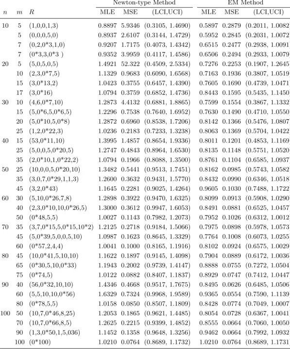
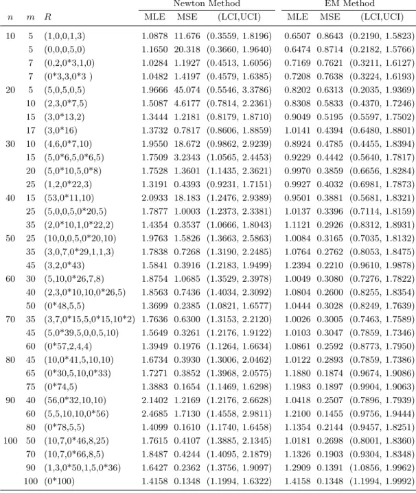
Step 6. Compute the MLE using the EM algorithm given in subsection 2.2. Now we discuss the results of a simulation study based on 5000 simulations to evaluate the MLE. The simulations were performed by using the R software. The sample sizes used in the simulation study are 10(10)100 and the values of β are 1.0 and 1.5 for different censoring schemes. The simulated values of MLE, mean squared error (MSE) and asymptotic confidence intervals forβ using Newton-type method and EM algorithm are presented in tables 1 and 2. It can be observed that in most cases the estimators obtained by the EM method converge to the true values of β better than that obtained by the Newton-type method. For the complete case, it can be noted that both methods converge to a very close estimate. A 95% confidence intervals for the parameter are constructed based on asymptotic variance. It is observed that the confidence intervals obtianed by Newton-type are wider than those obtained by EM algorithm. In general, we can not say that EM algorithm is always better than Newton-type method. This depends on the expectation of the log-likelihood function. A combination of the two methods, say Newton-EM, would give better results.
3.2 Data Analysis
For illustrative purpose, we use a data set corresponding to waiting times (in minutes) before service of 100 bank customers as discussed by Ghitany et al. (2008). The data are given as follows: 0.8, 0.8, 1.3, 1.5, 1.8, 1.9, 1.9, 2.1, 2.6, 2.7, 2.9, 3.1, 3.2, 3.3, 3.5, 3.6, 4.0, 4.1, 4.2, 4.2, 4.3, 4.3, 4.4, 4.4, 4.6, 4.7, 4.7, 4.8, 4.9, 4.9, 5.0, 5.3, 5.5, 5.7, 5.7, 6.1, 6.2, 6.2, 6.2, 6.3, 6.7, 6.9, 7.1, 7.1, 7.1, 7.1, 7.4, 7.6, 7.7, 8.0, 8.2, 8.6, 8.6, 8.6, 8.8, 8.8, 8.9, 8.9, 9.5, 9.6, 9.7, 9.8, 10.7, 10.9, 11.0, 11.0, 11.1, 11.2, 11.2, 11.5, 11.9, 12.4, 12.5, 12.9, 13.0, 13.1, 13.3, 13.6, 13.7, 13.9, 14.1, 15.4, 15.4, 17.3, 17.3, 18.1, 18.2, 18.4, 18.9, 19.0, 19.9, 20.6, 21.3, 21.4, 21.9, 23.0, 27.0, 31.6, 33.1, 38.5.
For analyzing this data set with progressively type-II censoring, we formulate different censoring schemes for different values ofm as shown in Table 3. Empirically, it can be observed from Table 3 that the MLEs obtained by the EM algorithm have the smallest standard errors (SE) as compared with that obtained by using Newton-type method. For fixed m, one can determine the censoring scheme that is most efficient from others.
4 Conclusion
In this study some results on statistical inference were developed using EM algorithm. Under the progressively type-II censoring scheme, we obtain the MLE for the unknown parameter for the Lindley distribution. The MCMC methods are used to generate sam-ple from Lindley distribution. The asymptotic variance of the MLE within the EM framework has been obtained. Consequently, the asymptotic confidence intervals of the parameter have been constructed. Comparisons are made between Newton-type method and EM algorithm via a simulation study. It has been observed in this study that
Newton-type Method EM Method
n m R MLE MSE (LCI,UCI) MLE MSE (LCI,UCI)
10 5 (1,0,0,1,3) 0.8897 5.9346 (0.3105, 1.4690) 0.5897 0.2879 (0.2011, 1.0082) 5 (0,0,0,5,0) 0.8937 2.6107 (0.3144, 1.4729) 0.5952 0.2845 (0.2031, 1.0072) 7 (0,2,0*3,1,0) 0.9207 1.7175 (0.4073, 1.4342) 0.6515 0.2477 (0.2938, 1.0091) 7 (0*3,3,0*3 ) 0.9352 3.9959 (0.4117, 1.4586) 0.6506 0.2494 (0.2933, 1.0079) 20 5 (5,0,5,0,5) 1.4921 52.322 (0.4509, 2.5334) 0.7276 0.2253 (0.1907, 1.2645) 10 (2,3,0*7,5) 1.1329 0.9683 (0.6090, 1.6568) 0.7163 0.1936 (0.3807, 1.0519) 15 (3,0*13,2) 1.0423 0.3755 (0.6457, 1.4390) 0.7605 0.1690 (0.4739, 1.0471) 17 (3,0*16) 1.0794 0.3759 (0.6852, 1.4736) 0.8443 0.1595 (0.5435, 1.1450) 30 10 (4,6,0*7,10) 1.2873 4.4132 (0.6881, 1.8865) 0.7599 0.1554 (0.3867, 1.1332) 15 (5,0*6,5,0*6,5) 1.2296 0.7538 (0.7640, 1.6952) 0.7630 0.1490 (0.4710, 1.0550) 20 (5,0*10,5,0*8) 1.2872 0.6960 (0.8538, 1.7206) 0.8142 0.1366 (0.5476, 1.0807) 25 (1,2,0*22,3) 1.0236 0.2183 (0.7233, 1.3238) 0.8063 0.1369 (0.5704, 1.0422) 40 15 (53,0*11,10) 1.3995 1.4857 (0.8654, 1.9336) 0.8011 0.1201 (0.4853, 1.1169) 25 (5,0,0,5,0*20,5) 1.2747 0.4843 (0.8964, 1.6530) 0.8135 0.1148 (0.5751, 1.0520) 35 (2,0*10,1,0*22,2) 1.0794 0.1966 (0.8088, 1.3500) 0.8761 0.1104 (0.6585, 1.0937) 50 25 (10,0,0,5,0*20,10) 1.3482 0.5441 (0.9513, 1.7451) 0.8162 0.0985 (0.5743, 1.0582) 35 (3,0,7,0*29,1,1,3) 1.2600 0.3632 (0.9431, 1.5770) 0.8432 0.0990 (0.6346, 1.0518) 45 (3,2,0*43) 1.1645 0.2281 (0.9025, 1.4264) 0.9605 0.1030 (0.7488, 1.1722) 60 30 (5,10,0*26,7,8) 1.2898 0.3922 (0.9470, 1.6325) 0.8099 0.0913 (0.5908, 1.0290) 40 (2,3,0*10,10,0*26,5) 1.3000 0.3612 (0.9947, 1.6053) 0.8491 0.0881 (0.6525, 1.0457) 50 (0*48,5,5) 1.0027 0.1143 (0.7982, 1.2073) 0.7952 0.1026 (0.6312, 1.0012) 70 35 (3,7,0*15,5,0*15,10*2) 1.2125 0.2718 (0.9184, 1.5066) 0.7975 0.0898 (0.5978, 1.0573) 45 (5,0*39,5,0,0,5,10) 1.0987 0.1623 (0.8645, 1.3329) 0.7764 0.1008 (0.6073, 1.0255) 60 (0*57,2,4,4) 1.0041 0.1000 (0.8165, 1.1916) 0.8102 0.0924 (0.6575, 1.0029) 80 45 (10,0*41,5,10,10) 1.1622 0.1897 (0.9145, 1.4098) 0.7904 0.0889 (0.6172, 1.0036) 65 (0*30,5,10,0*33) 1.1943 0.2002 (0.9739, 1.4147) 0.8888 0.0755 (0.7272, 1.0504) 75 (0*74,5) 1.0122 0.0882 (0.8407, 1.1837) 0.8929 0.0747 (0.7412, 1.0447) 90 40 (56,0*32,10,10) 1.4346 0.4668 (0.9517, 1.7675) 0.8495 0.0626 (0.6485, 1.0506) 60 (5,5,10,10,0*56) 1.6329 0.7324 (0.9968, 1.9589) 0.9365 0.0554 (0.7590, 1.1139) 80 (0*78,5,5) 1.0158 0.0850 (0.8507, 1.1809) 0.8428 0.0774 (0.7049, 1.0007) 100 50 (10,7,0*46,8,25) 1.2053 0.1865 (0.9621, 1.4485) 0.8054 0.0728 (0.6367, 1.0041) 70 (10,7,0*66,8,5) 1.2625 0.2215 (0.9399, 1.4852) 0.8555 0.0664 (0.7060, 1.0050) 90 (1,3,0*50,1,5,036) 1.1452 0.1358 (0.9648, 1.3256) 0.9462 0.0664 (0.7992, 1.0932) 100 (0*100) 1.0210 0.0764 (0.8689, 1.1732) 1.0210 0.0764 (0.8689, 1.1731)
Table 1: Average estimators, MSE and average asymptotic confidence intervals forβ = 1 at different values ofnand m under Newton-type method and EM algorithm.
Newton Method EM Method
n m R MLE MSE (LCI,UCI) MLE MSE (LCI,UCI)
10 5 (1,0,0,1,3) 1.0878 11.676 (0.3559, 1.8196) 0.6507 0.8643 (0.2190, 1.5823) 5 (0,0,0,5,0) 1.1650 20.318 (0.3660, 1.9640) 0.6474 0.8714 (0.2182, 1.5766) 7 (0,2,0*3,1,0) 1.0284 1.1927 (0.4513, 1.6056) 0.7169 0.7621 (0.3211, 1.6127) 7 (0*3,3,0*3 ) 1.0482 1.4197 (0.4579, 1.6385) 0.7208 0.7638 (0.3224, 1.6193) 20 5 (5,0,5,0,5) 1.9666 45.074 (0.5546, 3.3786) 0.8202 0.6313 (0.2035, 1.9369) 10 (2,3,0*7,5) 1.5087 4.6177 (0.7814, 2.2361) 0.8308 0.5833 (0.4370, 1.7246) 15 (3,0*13,2) 1.3444 1.2181 (0.8179, 1.8710) 0.9049 0.5195 (0.5597, 1.7502) 17 (3,0*16) 1.3732 0.7817 (0.8606, 1.8859) 1.0141 0.4394 (0.6480, 1.8801) 30 10 (4,6,0*7,10) 1.9550 18.672 (0.9862, 2.9239) 0.8924 0.4785 (0.4455, 1.8394) 15 (5,0*6,5,0*6,5) 1.7509 3.2343 (1.0565, 2.4453) 0.9229 0.4442 (0.5640, 1.7817) 20 (5,0*10,5,0*8) 1.7528 1.3601 (1.1435, 2.3621) 0.9970 0.3859 (0.6656, 1.8284) 25 (1,2,0*22,3) 1.3191 0.4393 (0.9231, 1.7151) 0.9927 0.4032 (0.6981, 1.7873) 40 15 (53,0*11,10) 2.0933 18.183 (1.2476, 2.9389) 0.9501 0.3881 (0.5681, 1.8321) 25 (5,0,0,5,0*20,5) 1.7877 1.0003 (1.2373, 2.3381) 1.0137 0.3396 (0.7114, 1.8159) 35 (2,0*10,1,0*22,2) 1.4354 0.3537 (1.0666, 1.8043) 1.1121 0.2926 (0.8312, 1.8931) 50 25 (10,0,0,5,0*20,10) 1.9763 1.5826 (1.3663, 2.5863) 1.0084 0.3165 (0.7035, 1.8132) 35 (3,0,7,0*29,1,1,3) 1.7838 0.7268 (1.3190, 2.2485) 1.0764 0.2762 (0.8053, 1.8475) 45 (3,2,0*43) 1.5841 0.3916 (1.2183, 1.9499) 1.2394 0.2210 (0.9610, 1.9878) 60 30 (5,10,0*26,7,8) 1.8754 1.0685 (1.3529, 2.3978) 1.0049 0.3080 (0.7276, 1.7822) 40 (2,3,0*10,10,0*26,5) 1.8563 0.7436 (1.4034, 2.3092) 1.0804 0.2600 (0.8255, 1.8354) 50 (0*48,5,5) 1.3699 0.2385 (1.0821, 1.6577) 1.0444 0.3028 (0.8249, 1.7639) 70 35 (3,7,0*15,5,0*15,10*2) 1.7636 0.6300 (1.3153, 2.2120) 1.0026 0.3005 (0.7463, 1.7589) 45 (5,0*39,5,0,0,5,10) 1.5649 0.3261 (1.2176, 1.9122) 1.0103 0.3047 (0.7859, 1.7346) 60 (0*57,2,4,4) 1.3949 0.1976 (1.1264, 1.6634) 1.0861 0.2592 (0.8773, 1.7950) 80 45 (10,0*41,5,10,10) 1.6734 0.3930 (1.3006, 2.0462) 1.0122 0.2893 (0.7859, 1.7386) 65 (0*30,5,10,0*33) 1.7271 0.3852 (1.3968, 2.0575) 1.1880 0.1874 (0.9674, 1.9086) 75 (0*74,5) 1.3883 0.1654 (1.1469, 1.6298) 1.1983 0.1897 (0.9904, 1.9063) 90 40 (56,0*32,10,10) 2.1402 1.2169 (1.2176, 2.6628) 1.0418 0.2507 (0.7896, 1.7939) 60 (5,5,10,10,0*56) 2.4685 1.7130 (1.4558, 2.9811) 1.2100 0.1455 (0.9756, 1.9444) 80 (0*78,5,5) 1.4099 0.1610 (1.1740, 1.6458) 1.1354 0.2144 (0.9457, 1.8251) 100 50 (10,7,0*46,8,25) 1.7615 0.4107 (1.3885, 2.1345) 1.0181 0.2698 (0.8001, 1.8360) 70 (10,7,0*66,8,5) 1.8487 0.4244 (1.4095, 2.1879) 1.1326 0.1903 (0.9304, 1.8348) 90 (1,3,0*50,1,5,0*36) 1.6427 0.2362 (1.3756, 1.9097) 1.2909 0.1391 (1.0856, 1.9962) 100 (0*100) 1.4158 0.1348 (1.1994, 1.6322) 1.4158 0.1348 (1.1994, 1.9992)
Table 2: Average estimators, MSE and average asymptotic confidence intervals forβ = 1.5 at different values ofn and munder Newton method and EM algorithm.
Newton-type Method EM Method
m R MLE SE (LCI,UCI) MLE SE (LCI,UCI)
50 (10,0*47,20,20) 0.2574 0.0236 (0.2112, 0.3036) 0.1862 0.0187 (0.1495, 0.2229) 70 (5,0*65,2,3,10,10) 0.2399 0.0193 (0.2020, 0.2777) 0.1717 0.0135 (0.1453, 0.1981) 90 (0*89,10) 0.2084 0.0153 (0.1785, 0.2383) 0.1665 0.0124 (0.1422, 0.1908) 100 (0*100) 0.1866 0.0133 (0.1605, 0.2126) 0.1866 0.0133 (0.1606, 0.2126) Table 3: MLE corresponding SE and 95% asymptotic confidence interval forβ at
differ-ent values ofm(observed data) under Newton-type method and EM algorithm.
the numerical MLEs obtained by the EM method converge to the true values of the unknown parameter better than those obtained by the Newton-type method. Also, it has been observed that the coverage probabilities for both methods are better when we had a larger number of observed data. Finally, a practical example has been analyzed for illustrative purpose. We have observed that the EM-algorithm and the Newtontype method produced very satisfactory results, but EM method provided better estimates. Therefore, we can conclude that EM algorithm seems a good procedure in estimation problem.
Acknowledgment
This study is a part of the Master Thesis of the second named author whose work was supervised by the first named author.
References
Al-Zahrani, B. and Gindwan, M. (2014). Parameter estimation of a two-parameter lind-ley distribution under hybrid censoring. International Journal of System Assurance Engineering and Management, 5(4):628–636.
Balakrishnan, N. and Aggarwala, R. (2000). Progressive censoring: theory, methods, and applications. Springer Science & Business Media.
Dempster, A. P., Laird, N. M., and Rubin, D. B. (1977). Maximum likelihood from incomplete data via the em algorithm. Journal of the royal statistical society. Series B (methodological), pages 1–38.
Geddes, K. O., Glasser, M. L., Moore, R. A., and Scott, T. C. (1990). Evaluation of classes of definite integrals involving elementary functions via differentiation of special functions. Applicable Algebra in Engineering, Communication and Computing, 1(2):149–165.
Ghitany, M., Alqallaf, F., Al-Mutairi, D., and Husain, H. (2011). A two-parameter weighted lindley distribution and its applications to survival data. Mathematics and Computers in Simulation, 81(6):1190–1201.
Ghitany, M., Atieh, B., and Nadarajah, S. (2008). Lindley distribution and its applica-tion. Mathematics and computers in simulation, 78(4):493–506.
Louis, T. A. (1982). Finding the observed information matrix when using the em al-gorithm. Journal of the Royal Statistical Society. Series B (Methodological), pages 226–233.
McLachlan, G. and Krishnan, T. (2007).The EM algorithm and extensions, volume 382. John Wiley & Sons.
Ng, H., Chan, P., and Balakrishnan, N. (2002). Estimation of parameters from progres-sively censored data using em algorithm. Computational Statistics & Data Analysis, 39(4):371–386.
Robert, C. and Casella, G. (2013). Monte Carlo statistical methods. Springer Science & Business Media.
Sarhan, A. M. and Abuammoh, A. (2008). Statistical inference using progressively type-ii censored data with random scheme. InInternational Mathematical Forum, volume 35, pages 1713–1725.
Shanker, R., Sharma, S., and Shanker, R. (2013). A two-parameter lindley distribution for modeling waiting and survival times data. Applied Mathematics, 4(02):363. Zakerzadeh, H. and Mahmoudi, E. (2012). A new two parameter lifetime distribution: