Memory PDE Solvers
by Nasir Touheed
Submitted in accordance with the requirements for the degree of Doctor of Philosophy
The University of Leeds School of Computer Studies
September 1998
The candidate conrms that the work submitted is his own and that appropriate credit has been given where reference has been made to the work of others.
Abstract
This thesis is concerned with the issue of dynamic load-balancing in connection with the parallel adaptive solution of partial dierential equations (PDEs). We are interested in parallel solutions based upon either nite element or nite volume schemes on unstructured grids and we assume that geometric parallelism is used, whereby the nite element or nite volume grids are partitioned across the available parallel processors. For parallel eciency it is necessary to maintain a well balanced partition and to attempt to keep communicationoverheads as low as possible. When adaptivity occurs however a given partition maydeteriorate in quality and so it must be modied dynamically. This is the problem that we consider in this work.
Chapters one and two outline the problem in more detail and review existing work in this eld. In Chapter one a brief history of parallel computers is presented and dierent kinds of parallel machines are mentioned. The nite elementmethod is also introduced and its parallel implementation is discussed in some detail: leading to the derivation of a static load-balancing problem. A number of important static load balancing algorithms are then discussed. Chapter two commences with a brief description of some error indicators and common techniques for mesh adaptivity. It is shown how this adaptivity may lead to a load imbalance among the available processors of a parallel machine. We then discuss some ways in which the static load-balancing algorithms of Chapter one can be modied and used in the context of dynamic load-balancing. The pros and cons of these strategies are discussed and then nally some specic dynamic load-balancing algorithms are introduced and discussed.
In Chapter three a new dynamic load-balancing algorithm is proposed based upon a number of generalisations of existing algorithms. The details of the new algorithm are outlined and a number of preliminary numerical experiments are un-dertaken. In this preliminary (sequential) version the dual graph of an existing partitioned computational mesh is repartioned among the same number of proces-sors so that after the repartitioning step each processor has an approximate equal load and the number of edges of this dual graph which cross from one processor to another are relatively small.
The remainder of the thesis is concerned with the practical parallel implemen-tation of this new algorithm and making comparison with existing techniques. In Chapter four the algorithm is implemented for a 2-d adaptive nite element solver
for steady-state problems, and in Chapter ve the generality of the implementation is enhanced and the algorithm is applied in conjunction with a 3-d adaptive nite volume solver for unsteady problems. In this situation frequent repartitioning of the mesh is required. In this chapter performance comparisons are made for the al-gorithm detailed here against new software that was developed simultaneously with the work of this thesis. These comparisons are very favourable for certain problems which involve very non-uniform renement.
All software implementations described in this thesis have been coded in ANSI C using MPI version 1.1 (where applicable). The Portability of the load-balancing code has been tested by making use of a variety of platforms, including a Cray T3D, an SGI PowerChallenge, dierent workstation networks (SGI Indys and SGI O2s), and an SGI Origin 2000. For the purposes of numerical comparisons all timings quoted in this thesis are for the SGI Origin 2000 unless otherwise stated.
Acknowledgements
I would like to thank my supervisor Dr. Peter Jimack for his guidance and encouragement throughout the course of this research. Not only was he very helpful in guiding me throughout my stay at Leeds, but he was also very patient when it came to correcting my poorly drafted chapters as regards to the English language. Thanks also to Dr. Martin Berzins, Dr. David Hodgson and Dr. Paul Selwood for their helpful advice and discussions during this time.
My thanks also go to the General Oce and Support sta of the School who were always happy to help me.
Thanks are also due to my colleagues Idrees Ahmad, Syed Shafaat Ali, Muham-mad Raq Asim, Fazilah Haron, Zahid Hussain, Jaw-Shyong Jan, Sharifullah Khan, Rashid Mahmood, Sarfraz Ahmad Nadeem, Allah Nawaz, Professor Muhammad Abdul-Rauf Quraishi, Shuja Muhammad Quraishi and Alex Tsai for matters not necessarily related to the research.
I would also like to acknowledge the Edinburgh Parallel Computing Centre at the University of Edinburgh for allowing me to use their parallel computing facilities, including the Cray T3D, and to thank Dr. Alan Wood of University of York, for his help and support in the early days of my stay in York.
Members of my extended family in Pakistan and of my immediate family here in the UK have been a great encouragement throughout the period of this research. I especially wish to thank my parents and sisters, brother-in-laws, mother-in-law and father-in-law for their encouragement. My two daughters Maryam and Sidrah (who was a much needed and welcome addition to our family in the middle of this project) have been most patient while I nished this task. This project would not have been completed without the constant love and support of my wife, Shagufta.
Finally, my thanks also go to the University of Karachi, the Government of Pakistan and the Committee of Vice-Chancellors and Principals of the Universities of the United Kingdom for supporting me nancially throughout my research in the forms of Study-Leave, COTS and ORS Awards respectively.
At the very end I would like to thank The Almighty,for the much needed courage and strength which He granted me at this relatively old age of my life to nalise the project.
Contents
1 Introduction
1
1.1 Introduction to Parallel Computers : : : : : : : : : : : : : : : : : : 3 1.1.1 SIMD Systems : : : : : : : : : : : : : : : : : : : : : : : : : 4 1.1.2 General MIMD Systems : : : : : : : : : : : : : : : : : : : : 4 1.2 Comparison Between SIMD and MIMD Computers : : : : : : : : : 7 1.3 Finite Element Methods for Elliptic PDEs : : : : : : : : : : : : : : 9 1.3.1 Piecewise Linear Finite Elements : : : : : : : : : : : : : : : 11 1.3.2 Algorithmic Details : : : : : : : : : : : : : : : : : : : : : : : 12 1.4 Time-Dependent Problems: The Linear Diusion Equation : : : : : 15 1.4.1 The Method of Lines : : : : : : : : : : : : : : : : : : : : : : 15 1.5 Parallel Finite Element and Load-Balancing : : : : : : : : : : : : : 17 1.6 Recursive Graph Partitioning Heuristics : : : : : : : : : : : : : : : 20 1.6.1 Recursive Coordinate Bisection (RCB) : : : : : : : : : : : : 20 1.6.2 Recursive Inertial Bisection (RIB) : : : : : : : : : : : : : : : 21 1.6.3 Recursive Graph Bisection (RGB) : : : : : : : : : : : : : : : 21 1.6.4 Modied Recursive Graph Bisection (MRGB) : : : : : : : : 21 1.6.5 Recursive Spectral Bisection (RSB) : : : : : : : : : : : : : : 22 1.6.6 Recursive Node Cluster Bisection (RNCB) : : : : : : : : : : 23 1.7 Multisectional Graph Partitioning Heuristics : : : : : : : : : : : : : 24 1.7.1 Multidimensional Spectral Graph Partitioning : : : : : : : : 25 1.7.2 Stripwise Methods : : : : : : : : : : : : : : : : : : : : : : : 25 1.8 Other Graph Partitioning Techniques : : : : : : : : : : : : : : : : : 25 1.8.1 Greedy Algorithm (GR) : : : : : : : : : : : : : : : : : : : : 25 1.8.2 Kernighan and Lin Type Algorithms : : : : : : : : : : : : : 26 1.8.3 State of the Art Software Tools for Graph Partitioning : : : 26
2 Adaptivity and Dynamic Load Balancing
29
2.1 Spatial Error Indicators : : : : : : : : : : : : : : : : : : : : : : : : 30 2.2 Dierent Types of Renements : : : : : : : : : : : : : : : : : : : : 31 2.2.1 Regeneration Schemes : : : : : : : : : : : : : : : : : : : : : 31 2.2.2 Local Mesh Adaptation Schemes : Hierarchical Renement : 32 2.3 Relation Between Adaptivity and Dynamic Load Balancing : : : : : 34 2.3.1 Generalisations of Static Algorithms : : : : : : : : : : : : : 36 2.4 Diusion Algorithms : : : : : : : : : : : : : : : : : : : : : : : : : : 39 2.4.1 Basic Diusion Method: : : : : : : : : : : : : : : : : : : : : 40 2.4.2 A Multi-Level Diusion Method : : : : : : : : : : : : : : : : 40 2.4.3 Dimension Exchange Method : : : : : : : : : : : : : : : : : 42 2.5 Minimising Data Migration : : : : : : : : : : : : : : : : : : : : : : 43 2.6 Two Parallel Multilevel Algorithms : : : : : : : : : : : : : : : : : : 45 2.6.1 ParMETIS: : : : : : : : : : : : : : : : : : : : : : : : : : : : 45 2.6.2 ParJOSTLE : : : : : : : : : : : : : : : : : : : : : : : : : : : 46 2.7 Two Further Paradigms : : : : : : : : : : : : : : : : : : : : : : : : 47 2.7.1 Algorithm of Oliker & Biswas : : : : : : : : : : : : : : : : : 47 2.7.2 Algorithm of Vidwans et al. : : : : : : : : : : : : : : : : : : 48
3 A New Dynamic Load Balancer
50
3.1 Motivation of the Algorithm : : : : : : : : : : : : : : : : : : : : : : 51 3.2 Description of the Algorithm: : : : : : : : : : : : : : : : : : : : : : 51 3.2.1 Group Balancing : : : : : : : : : : : : : : : : : : : : : : : : 52 3.2.2 Local Migration : : : : : : : : : : : : : : : : : : : : : : : : : 53 3.3 Further Renement of the Algorithm : Locally Improving the
Parti-tion Quality : : : : : : : : : : : : : : : : : : : : : : : : : : : : : : : 56 3.4 Global Load-Balancing Strategy: Divide and Conquer Approach : : 58 3.5 Examples : : : : : : : : : : : : : : : : : : : : : : : : : : : : : : : : 60 3.6 Conclusions : : : : : : : : : : : : : : : : : : : : : : : : : : : : : : : 73
4 Parallel Application of the Dynamic Load Balancer in 2-d
77
4.1 Introduction : : : : : : : : : : : : : : : : : : : : : : : : : : : : : : : 79 4.2 A Parallel Dynamic Load-Balancing Algorithm: : : : : : : : : : : : 80 4.2.1 Group Balancing : : : : : : : : : : : : : : : : : : : : : : : : 81
4.2.2 Local Migration : : : : : : : : : : : : : : : : : : : : : : : : : 82 4.2.3 Divide and Conquer and Parallel Implementation : : : : : : 84 4.3 Discussion of the Algorithm : : : : : : : : : : : : : : : : : : : : : : 87 4.3.1 Activity of Type 1 Processors : Packing the Load : : : : : : 88 4.3.2 Activity of Type 2 Processors : Unpacking the Load: : : : : 88 4.3.3 Activity of Type 3 Processors : Third Party Adjustment : : 88 4.4 Description of Related Data Structures Associated With the
Redis-tribution of the Mesh : : : : : : : : : : : : : : : : : : : : : : : : : : 89 4.5 Dierent Issues and Related Functions Used in the Main Algorithm
By Processors of Type 1 : : : : : : : : : : : : : : : : : : : : : : : : 93 4.5.1 Handling of Vertices : : : : : : : : : : : : : : : : : : : : : : 93 4.5.2 Handling of Edges : : : : : : : : : : : : : : : : : : : : : : : 95 4.6 Dierent Issues Which are Related With Processors of Type 2 : : : 100 4.7 Dierent Issues Which are Related With Processors of Type 3 : : : 101 4.7.1 insertion() : : : : : : : : : : : : : : : : : : : : : : : : : : : : 101 4.7.2 deletion() : : : : : : : : : : : : : : : : : : : : : : : : : : : : 101 4.8 Use of Message Passing Interface (MPI): : : : : : : : : : : : : : : : 101 4.9 Some Examples : : : : : : : : : : : : : : : : : : : : : : : : : : : : : 103 4.9.1 Alternative Algorithms : : : : : : : : : : : : : : : : : : : : : 103 4.9.2 Comparative Results : : : : : : : : : : : : : : : : : : : : : : 105 4.10 Discussion : : : : : : : : : : : : : : : : : : : : : : : : : : : : : : : : 121 4.10.1 Discussion I : : : : : : : : : : : : : : : : : : : : : : : : : : : 121 4.10.2 Discussion II : : : : : : : : : : : : : : : : : : : : : : : : : : 122 4.11 Conclusions : : : : : : : : : : : : : : : : : : : : : : : : : : : : : : : 123
5 Parallel Application of the Dynamic Load Balancer in 3-d
125
5.1 Introduction : : : : : : : : : : : : : : : : : : : : : : : : : : : : : : : 126 5.2 A Parallel Adaptive Flow Solver : : : : : : : : : : : : : : : : : : : : 128 5.2.1 A Parallel Adaptive Algorithm : : : : : : : : : : : : : : : : 128 5.2.2 A Parallel Finite Volume Solver : : : : : : : : : : : : : : : : 131 5.3 Dynamic Load Balancing : : : : : : : : : : : : : : : : : : : : : : : : 132 5.4 Application of the Parallel Dynamic Load-Balancing Algorithm : : 133 5.4.1 Calculation of WPCG : : : : : : : : : : : : : : : : : : : : : 133 5.4.2 Use of Tokens : : : : : : : : : : : : : : : : : : : : : : : : : : 134
5.4.3 No Colouring : : : : : : : : : : : : : : : : : : : : : : : : : : 135 5.4.4 Use of Global Communication : : : : : : : : : : : : : : : : : 136 5.5 Computational Results : : : : : : : : : : : : : : : : : : : : : : : : : 137 5.5.1 Examples : : : : : : : : : : : : : : : : : : : : : : : : : : : : 138 5.6 Discussion : : : : : : : : : : : : : : : : : : : : : : : : : : : : : : : : 150 5.6.1 Discussion I : : : : : : : : : : : : : : : : : : : : : : : : : : : 150 5.6.2 Discussion II : : : : : : : : : : : : : : : : : : : : : : : : : : 152 5.7 Investigation into Scalability of the Algorithm : : : : : : : : : : : : 154 5.8 Conclusions : : : : : : : : : : : : : : : : : : : : : : : : : : : : : : : 160
6 Conclusion and Future Areas of Research
161
6.1 Summary of Thesis : : : : : : : : : : : : : : : : : : : : : : : : : : : 161 6.2 Possible Extensions to the Research : : : : : : : : : : : : : : : : : : 162
List of Figures
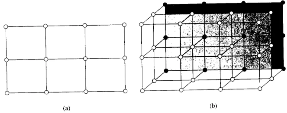
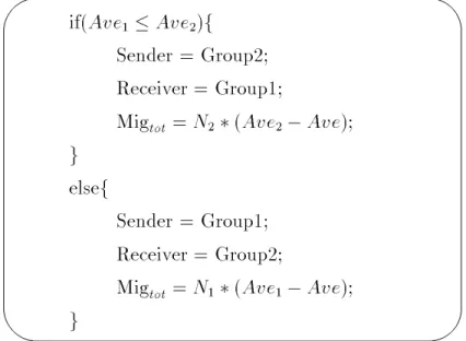
1.1 A linear array of processors. : : : : : : : : : : : : : : : : : : : : : : 6 1.2 A ring of processors. : : : : : : : : : : : : : : : : : : : : : : : : : : 6 1.3 Hypercubes of (a) dimension 1, (b) dimension 2 and (c) dimension 3. 7 1.4 (a) Two-dimensional mesh, (b) three-dimensional mesh. : : : : : : : 8 1.5 Two-dimensional torus. : : : : : : : : : : : : : : : : : : : : : : : : : 8 1.6 Entries of the Laplacian matrix. : : : : : : : : : : : : : : : : : : : : 23 2.1 Diusion method. : : : : : : : : : : : : : : : : : : : : : : : : : : : : 41 2.2 Multi-level diusion method. : : : : : : : : : : : : : : : : : : : : : : 42 2.3 Dimension exchange method. : : : : : : : : : : : : : : : : : : : : : 43 2.4 The matrix A. : : : : : : : : : : : : : : : : : : : : : : : : : : : : : : 44 3.1 Calculation of Sender, Receiver and Migtot: : : : : : : : : : : : : : : 54
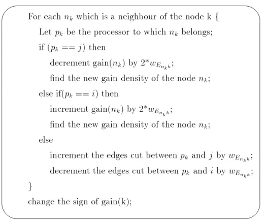
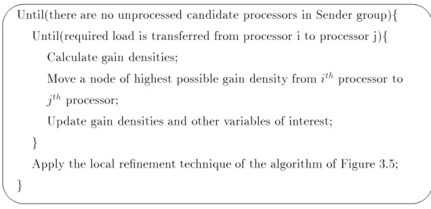
3.2 The calculation of gain. : : : : : : : : : : : : : : : : : : : : : : : : : 55 3.3 Updation of gain densities and edges cut between the processors. : : 56 3.4 Initial version of load balancing of the two groups. : : : : : : : : : : 57 3.5 An algorithm for rening the partitions between a pair of processors. 58 3.6 Group-balancing algorithm: version two of load balancing of the two
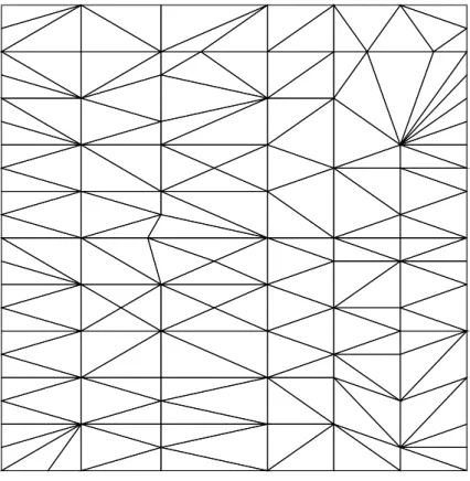
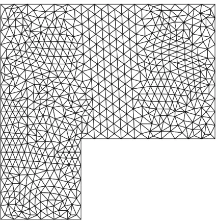
groups. : : : : : : : : : : : : : : : : : : : : : : : : : : : : : : : : : : 59 3.7 A divide & conquer type dynamic load-balancing algorithm. : : : : 61 3.8 The coarse mesh of Example 1. : : : : : : : : : : : : : : : : : : : : 63 3.9 The coarse mesh of Example 2. : : : : : : : : : : : : : : : : : : : : 65 3.10 The coarse \Texas" mesh of Example 4. : : : : : : : : : : : : : : : 69 3.11 Coarse mesh of 5184 elements adapted to initial shock condition for
Example 5. : : : : : : : : : : : : : : : : : : : : : : : : : : : : : : : 72 3.12 Adapted mesh after 240 time-steps for Example 5. : : : : : : : : : : 72 4.1 Updating the gains. : : : : : : : : : : : : : : : : : : : : : : : : : : : 84
4.2 Load balancing of the two groups. : : : : : : : : : : : : : : : : : : : 85 4.3 Parallel dynamic load-balancing algorithm. : : : : : : : : : : : : : : 86 4.4 The arraynonodessuballwhich can accommodate nine coarse elements. 92 4.5 The functionShared(). : : : : : : : : : : : : : : : : : : : : : : : : : 94 4.6 The functionShared2(). : : : : : : : : : : : : : : : : : : : : : : : : 94 4.7 The functionChangenbhd(). : : : : : : : : : : : : : : : : : : : : : : 96 4.8 The functionChangenbhd2(). : : : : : : : : : : : : : : : : : : : : : 97 4.9 The functionChangenbhd3(). : : : : : : : : : : : : : : : : : : : : : 98 4.10 The functionEdgeChange(). : : : : : : : : : : : : : : : : : : : : : : 99 4.11 The functionDirichEdgeChange().: : : : : : : : : : : : : : : : : : : 100 4.12 The coarse mesh of Example 3. : : : : : : : : : : : : : : : : : : : : 108 4.13 The partial view of the coarse mesh of Example 4. : : : : : : : : : : 109 5.1 Mesh data-structures in TETRAD : : : : : : : : : : : : : : : : : : 129 5.2 Regular renement dissecting interior diagonal : : : : : : : : : : : : 130 5.3 Green renement by the addition of an interior node : : : : : : : : 131 5.4 Calculation of weights of vertices and edges of the weighted dual graph.135 5.5 Calculation of a row of the weighted Laplacian matrix. : : : : : : : 136 5.6 Scalability comparison using a re-balancing tolerance of 5% for
Ex-ample 1 (where Time = RedTime + SolTime). : : : : : : : : : : : : 155 5.7 Scalability comparison using a re-balancing tolerance of 10% for
Ex-ample 1 (where Time = RedTime + SolTime). : : : : : : : : : : : : 155 5.8 Scalability comparison using a re-balancing tolerance of 15% for
Ex-ample 1 (where Time = RedTime + SolTime). : : : : : : : : : : : : 155 5.9 Scalability comparison using a re-balancing tolerance of 5% for
Ex-ample 2 (where Time = RedTime + SolTime). : : : : : : : : : : : : 156 5.10 Scalability comparison using a re-balancing tolerance of 10% for
Ex-ample 2 (where Time = RedTime + SolTime). : : : : : : : : : : : : 156 5.11 Scalability comparison using a re-balancing tolerance of 15% for
Ex-ample 2 (where Time = RedTime + SolTime). : : : : : : : : : : : : 156 5.12 Scalability comparison using a re-balancing tolerance of 15% for
Ex-ample 1 (where Time = RedTime + 0.2 * SolTime).: : : : : : : : : 157 5.13 Scalability comparison using a re-balancing tolerance of 15% for
5.14 Scalability comparison using a re-balancing tolerance of 15% for Ex-ample 1 (where Time = RedTime + 25 * SolTime). : : : : : : : : : 157 5.15 Scalability comparison using a re-balancing tolerance of 15% for
Ex-ample 2 (where Time = RedTime + 0.2 * SolTime).: : : : : : : : : 158 5.16 Scalability comparison using a re-balancing tolerance of 15% for
Ex-ample 2 (where Time = RedTime + 5 * SolTime).: : : : : : : : : : 158 5.17 Scalability comparison using a re-balancing tolerance of 15% for
List of Tables
3.1 Partition generated in parallel on 8 processors along with our nal partitions for Example 1. : : : : : : : : : : : : : : : : : : : : : : : : 64 3.2 Summary of results when the New, Vidwanset al., Chaco and
JOS-TLE algorithms are applied to the initial partition (see Table 3.1) of Example 1. : : : : : : : : : : : : : : : : : : : : : : : : : : : : : : : 64 3.3 Partition generated in parallel on 8 processors along with our nal
partitions for Example 2. : : : : : : : : : : : : : : : : : : : : : : : : 66 3.4 Summary of results when the New, Vidwanset al., Chaco and
JOS-TLE algorithms are applied to the initial partition (see Table 3.3) of Example 2. : : : : : : : : : : : : : : : : : : : : : : : : : : : : : : : 66 3.5 Partition generated in parallel on 8 processors along with our nal
partitions for Example 3. : : : : : : : : : : : : : : : : : : : : : : : : 68 3.6 Summary of results when the New, Vidwanset al., Chaco and
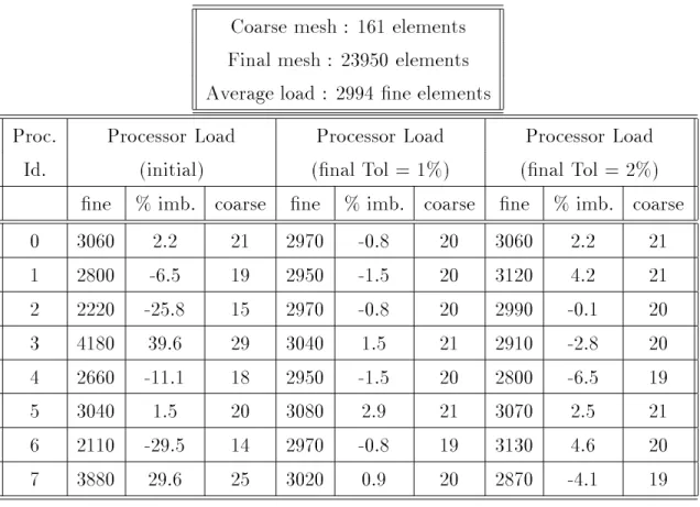
JOS-TLE algorithms are applied to the initial partition (see Table 3.5) of Example 3. : : : : : : : : : : : : : : : : : : : : : : : : : : : : : : : 68 3.7 Partition generated in parallel on 16 processors along with our nal
partitions for Example 4. : : : : : : : : : : : : : : : : : : : : : : : : 70 3.8 Summaryof results when the New, Vidwanset al. and JOSTLE
algo-rithms are applied to the initial partition (see Table 3.7) of Example 4. : : : : : : : : : : : : : : : : : : : : : : : : : : : : : : : : : : : : : 70 3.9 Initial and nal partitions (produced by the New algorithm) for
Ex-ample 5. : : : : : : : : : : : : : : : : : : : : : : : : : : : : : : : : : 73 3.10 Summary of results when the New, Vidwanset al., Chaco and
JOS-TLE algorithms are applied to the initial partition (see Table 3.9) of Example 5. : : : : : : : : : : : : : : : : : : : : : : : : : : : : : : : 73
3.11 Initial and nal partitions (produced by the New algorithm) for Ex-ample 6. : : : : : : : : : : : : : : : : : : : : : : : : : : : : : : : : : 74 3.12 Summary of results when the New, Vidwanset al., Chaco and
JOS-TLE algorithms are applied to the initial partition (see Table 3.11) of Example 6. : : : : : : : : : : : : : : : : : : : : : : : : : : : : : : 74 4.1 Data for the partitions of Example 1 (involving parallel mesh
gener-ation and repartitioning on 2 processors). : : : : : : : : : : : : : : : 107 4.2 Data for the partitions of Example 2 (involving parallel mesh
gener-ation and repartitioning on 4 processors). : : : : : : : : : : : : : : : 107 4.3 Data for the partitions of Example 3 (involving parallel mesh
gener-ation and repartitioning on 4 processors). : : : : : : : : : : : : : : : 109 4.4 Data for the partitions of Example 4 (involving parallel mesh
gener-ation and repartitioning on 4 processors). : : : : : : : : : : : : : : : 110 4.5 Data for the partitions of Example 5 (involving parallel mesh
gener-ation and repartitioning on 2 processors). : : : : : : : : : : : : : : : 110 4.6 Data for the partitions of Example 6 (involving parallel mesh
gener-ation and repartitioning on 4 processors). : : : : : : : : : : : : : : : 111 4.7 Comparison of dynamic load-balancing results using four algorithms
for Examples 1 to 6. : : : : : : : : : : : : : : : : : : : : : : : : : : 112 4.8 Data for the partitions of Example 7 (involving parallel mesh
gener-ation and repartitioning on 8 processors). : : : : : : : : : : : : : : : 113 4.9 Data for the partitions of Example 8 (involving parallel mesh
gener-ation and repartitioning on 16 processors). : : : : : : : : : : : : : : 115 4.10 Data for the partitions of Example 9 (involving parallel mesh
gener-ation and repartitioning on 8 processors). : : : : : : : : : : : : : : : 116 4.11 Data for the partitions of Example 10 (involving parallel mesh
gen-eration and repartitioning on 16 processors). : : : : : : : : : : : : : 117 4.12 Data for the partitions of Example 11 (involving parallel mesh
gen-eration and repartitioning on 8 processors). : : : : : : : : : : : : : : 118 4.13 Data for the partitions of Example 12 (involving parallel mesh
gen-eration and repartitioning on 16 processors). : : : : : : : : : : : : : 119 4.14 Comparison of dynamic load-balancing results using four algorithms
5.1 Some partition-quality metrics immediately before and after a single re-balancing step for Example 1. : : : : : : : : : : : : : : : : : : : : 141 5.2 Solution times, redistribution times, total migration weights and
mi-gration frequencies for 300 time-steps using a re-balancing tolerance of 5% for Example 1. : : : : : : : : : : : : : : : : : : : : : : : : : : 142 5.3 Solution times, redistribution times, total migration weights and
mi-gration frequencies for 300 time-steps using a re-balancing tolerance of 10% for Example 1. : : : : : : : : : : : : : : : : : : : : : : : : : 143 5.4 Solution times, redistribution times, total migration weights and
mi-gration frequencies for 300 time-steps using a re-balancing tolerance of 15% for Example 1. : : : : : : : : : : : : : : : : : : : : : : : : : 144 5.5 Some partition-quality metrics immediately before and after a single
re-balancing step for Example 2. : : : : : : : : : : : : : : : : : : : : 146 5.6 Solution times, redistribution times, total migration weights and
mi-gration frequencies for 300 time-steps using a re-balancing tolerance of 5% for Example 2. : : : : : : : : : : : : : : : : : : : : : : : : : : 147 5.7 Solution times, redistribution times, total migration weights and
mi-gration frequencies for 300 time-steps using a re-balancing tolerance of 10% for Example 2. : : : : : : : : : : : : : : : : : : : : : : : : : 148 5.8 Solution times, redistribution times, total migration weights and
mi-gration frequencies for 300 time-steps using a re-balancing tolerance of 15% for Example 2. : : : : : : : : : : : : : : : : : : : : : : : : : 149
Chapter 1
Introduction
Since the middle of the current century, breakthroughs in computer technology have made a tremendous impact on numerical methods in general and the numerical solutions of partial dierential equations in particular. During the infancy period of computers they were serial in nature. This means that they were built using the von Neumann paradigm: with a single processor which runs as fast as possible and has as much memory as is possible (or aordable). The processor is commonly known as the central processing unit (CPU) and is further divided into a control unit and an arithmetic-logic unit (ALU). The memory stores both instructions and data. The control unit directs the execution of programs, and the ALU carries out the calculations called for in the program. When they are being used by the program, instructions and data are stored in very fast memory locations, called registers. As fast memory is quite expensive, there are relatively few registers.
The performance of such computers is clearly limited by physical laws. For example, the maximum speed at which the data can travel from memory to CPU is that of the speed of light, so in order to build a computer which is capable of carrying out three trillion copies of data between memory and registers per second say, one has to t each 32-bit word into a square with side length of 10?10 meters
(this is approximately equal to the size of a relatively small atom). This is simply not possible - see [79] for details.
In order to speed up the machine, one possibility is to reduce the transfer time taken by the data while travelling from memory to registers. This is achieved by the use of cache memory - which is implemented on the same chip as the CPU. The idea behind cache is the observation that programs tend to access both data and
instructions sequentially. Hence, if we store a small block of data and a small block of instructions in fast memory (cache), most of the program's memory accesses will use this cache memory rather than the slower main memory. This memory will be slower than registers but it will be faster than the main memory implemented outside the chip.
During the initial stages in the development of microchips, designers typically used an increased chip area to introduce new and sophisticated instructions, ad-dressing modes and other mechanisms. These new features allowed the execution of high-level languages as well as the complex functions of operating systems, and this trend continued until the 1980s. At this time a new design philosophy called the reduced instruction set computer (RISC) emerged. The RISC supporters argue that all these new instructions complicate the design of the control unit, slowing down the execution of basic operations. A simple instruction set allows, in principle, a simple, fast implementation, so the larger number of instructions that is require can be more than compensated for by the increased speed. Another advantage claimed by RISC supporters is that the simplication of the control unit helps to save chip area for the control implementation. This can be used to implement special features in the operating unit, aimed at improving the execution speed. There are many variants of RISC processors, among them are Berkeley RISC, microprocessors with-out interlocked pipe stages (MIPS) and the Inmos Transputer (see Chapter 10 of [20]).
Even after all these advancements in the development of the computer industry there were and still are important classes of problem in science and engineering which practitioners have not been able to solve successfully. For example, to attack the \Grand Challenges" ([17]) months or even years are needed by the best of these computers. A grand challenge is a fundamental problem in science or engineering that has a broad economic and scientic impact, and whose solution could be ad-vanced by applying high-performance computing techniques and resources ([67]). Many of these problems are basically large computational uid dynamics problems which can be modelled by a set of partial dierential equations (PDEs).
To have an idea of the computing requirements to solve such problems numer-ically we consider here two examples. The rst one is studied by Case et al. ([16]) as mentioned in [26]. This is the simulation of a three-dimensional, fully resolved, turbulent ow as might occur in the design of a portion of a ship hull. The primary
parameter for characterising the turbulent uid ow is the dimensionless quantity known as the Reynolds number (R). Such a simulation would have a Reynolds num-ber of about 104 or greater. In order to fully resolve important disturbances of a
small wave number in the ow one needsR9=4 mesh points ([21]). That is N = 109
mesh points for each time step. Each mesh point has one pressure term and three velocity terms for both the current and the immediate past time step. This is a total of 8 10
9 scalar variables. If temperature or other parameters must also be
maintained for each point, then about 1010 words of data memory are required. The
number of arithmetic operations varies widely, depending upon the solution method employed. One ecient approach that takes advantage of the problem geometry, has been estimated to require only about 500 additions and 300 multiplications per grid point. This leads to an operations count of 10
12 operations per single time
step (see [26] for details).
The second problem is that of modeling and forecasting of weather. Suppose we want to predict the weather over an area of 3000 3000 miles for two-day period
and the parameters need to computed once every half hour. As mentioned in [67], if the area is being modeled up to a height of 11 miles and one wishes to partition this 3000 3000 11 cubic mile domain into segments of size 0.1 0.1 0.1
then there would be 1011 dierent segments. So we need at least 1011 words of data
memory. It is also estimated in [67] that for this prediction the total number of operations is 1015.
The world's most powerful computer of the mid 70's was the CRAY-1, which was not even close to having enough capability ([84]) to perform these calculations. It's primary memory was limited to 106 words, and the execution rate was about
108 operations/second.
Hence by this time it was clear that new, more powerful computer systems would be needed to solve this class of problems. Since the single processor machines had begun to start approaching its physical limits, the community had no choice but to consider alternative paradigms such as parallel machines.
1.1 Introduction to Parallel Computers
Parallel computers perform their calculations by executing dierent computational tasks on a number of processors concurrently. The processors within a parallel
computer generally exchange information during the execution of the parallel code. This exchange of information occurs either in the form of explicit messages sent by one processor to another or dierent parallel processors sharing a specied com-mon memory resource within the parallel computer. The parallel load-balancing algorithms, proposed in this thesis, work very well on these paradigms.
In 1966 Michael Flynn ([33]) classied systems according to the number of in-struction streams and the number of data streams. The two important systems are:
SIMD - Single Instruction stream, Multiple Data stream, MIMD - Multiple Instruction stream, Multiple Data stream.
This section provides a brief introduction to these important classes of parallel computing architecture.
1.1.1 SIMD Systems
Such a system has a single CPU devoted to exclusively to control, and a large collection of subordinate processors, each having only ALUs, and their own (small amount of) memory. During each instruction cycle, the control processor broadcasts an instruction to all of the subordinate processors, and each of the subordinate processors either executes the instruction or is idle.
The most famous examples of SIMD machines are the CM-1 and CM-2 connec-tion Machines that were produced by Thinking Machines. The CM-2 had up to 65,356 1-bit processors and up to 8 billion bytes of memory. Maspar also produced SIMD machines. The MP-2 has up to 16,384 32-bit ALUs and up to 4 billion bytes of memory.
1.1.2 General MIMD Systems
The key dierence between MIMD and SIMD systems is that with MIMD systems, the processors are autonomous: each processor is a full-edged CPU with both a control unit and an ALU. Thus each processors is capable of executing its own program at its own pace. The world of MIMD systems is divided into shared-memory and distributed-shared-memory systems.
Shared-Memory MIMD
A generic shared-memory machine consists of a collection of processors and memory modules interconnected by a network. Each processor has access to the entire address space of the memory modules. So that any data stored in the shared memory is common to, and can be accessed by, any of the processors. This has the advantage of being very rapid (in principle) and is generally simpler to program. However, its main drawback is that there can be serious delays (contention time) if more than one processor wants to use the same location in memory at the same time. The simplest network connection is bus based. Due to the limited bandwidth of a bus, these architectures do not scale to large number of processors: the largest conguration of the currently popular SGI Challenge XL has only 36 processors. Recently Silicon Graphics, Inc. has designed and manufactured the Origin 2000 computer. The basic building block of the Origin is a node built upon two MIPS R10000 processors with a peak performance of 400 Mop each. The computer utilises Scalable Shared-memory MultiProcessing (S2MP) architecture. Most other shared-memory architectures rely on some type of switch-based interconnection network. For example the basic unit of the Convex SPP1200 is a 5 5 crossbar
switch.
Distributed-Memory MIMD
In distributed-memory systems, each processor has its own private memory. These processors are connected directly or indirectly by means of communication wires. From the performance and programming point of view the ideal interconnection network is a fully connected network, in which each processor is directly connected to every other processor. Unfortunately, the exponential growth in the size (and cost) of such a network makes it impractical to construct such a machine with more than a few processors. At the opposite extreme from a fully connected network is a
linear array
: a static network in which all but two of the processors have two immediately adjacent neighbouring processors (see Figure 1.1). Aring
is a slightly more powerful network. This is just a linear array in which \terminal" processors have been joined (see Figure 1.2). These networks are relatively inexpensive; the only additional cost is the cost of p - 1 or p wires for a network of p processors. Moreover it is very cheap to upgrade the network - to add one processor we onlyFigure 1.1: A linear array of processors.
Figure 1.2: A ring of processors. need one extra wire. There are two principal drawbacks:
if two processors are communicating, it's very likely that this will prevent
other processors which are also attempting to communicate from doing so,
in a linear array two processors that are attempting to communicate may have
to forward the message along as many as p - 1 wires, and in a ring it may be necessary to forward the message along as many as p/2 wires.
In between the two extremes a
hypercube
is a practical static interconnection network that gives a good balance between the high cost and high speed of the fully connected network and the low cost but poor performance of the linear array or ring. Hypercubes are dened inductively: a dimension 0 hypercube consists of a single processor. In order to construct a hypercube of dimension d > 0, we take two hypercubes of dimensiond?1 and join the corresponding processors withFigure 1.3: Hypercubes of (a) dimension 1, (b) dimension 2 and (c) dimension 3. d will consist of 2d processors. It is also clear that in a hypercube of dimension
d each processor is directly connected to d other processors and that if we follow the shortest path then the maximum number of wires a message has to travel is d. This is much few than for the linear array of ring. The principal drawback to the hypercube is that it is not easy to upgrade the system : each time we wish to increase the machine size, we must double the number of processors and add a new wire to each processor. The rst \massively parallel" MIMD system was a hypercube (an nCUBE 10 with 1024 processors).
Intermediate between hypercubes and linear arrays are the
meshes
andtori
(see Figures 1.4 and 1.5), which are simply higher dimensional analogues of linear arrays and rings, respectively. Observe that an n-dimensional torus can be obtained from the n-dimensional mesh by adding \wrap-around" wires to the processors on the border. As far as upgrading is concerned meshes and tori are better than hypercubes (although not as good as linear arrays and rings). For example, if one wishes to increase the size of a q q mesh, one simply adds a q 1 meshand q wires. Meshes and tori are currently quite popular. The Intel Paragon is a two-dimensional mesh, and the Cray T3D and T3E are both three-dimensional tori.
1.2 Comparison Between SIMD and MIMD
Com-puters
In [67], Kumar et al. discuss the pros and cons of SIMD and MIMD computers. SIMD computers require less hardware and less memory than MIMD computers
Figure 1.4: (a) Two-dimensional mesh, (b) three-dimensional mesh.
because they have only one global control unit and only one copy of the program needs to be stored. On the other hand, MIMD computers store the program and operating system at each processor. SIMD computers are naturally suited for data-parallel programs; that is, programs in which the same set of instructions are ex-ecuted on a large data set (which is the case in the eld of image processing for example).
A clear disadvantage of SIMD computers is that dierent processors cannot execute dierent instructions in the same clock cycle, so if a program has many conditional branches or long segments of code whose execution depends on condi-tionals, it is entirely possible that many processors will remain idle for long periods of time. Data-parallel programs in which signicant parts of the computation are contained in conditional statements are therefore better suited to MIMD computers than to SIMD computers.
Individual processors in an MIMD computer are more complex, because each processors has its own control unit. It may seem that the cost of each processor must be higher than the cost of a SIMD processor. However, it is possible to use general-purpose microprocessors as processing units in MIMD computers. In contrast, the CPU used in SIMD computers has to be specially designed. Hence, due to economies of scale, processors in MIMD computers may be both cheaper and more powerful than processors in SIMD computers.
1.3 Finite Element Methods for Elliptic PDEs
Probably the three most popular numericaltechniques for solving partial dierential equations are the nite dierence, the nite element and the nite volume methods. In the nite dierence approximation, the derivatives in a dierential equation are replaced by dierence quotients. The dierence operators are usually derived from Taylor series and involve the values of the solution at neighbouring points in the domain. After taking the boundary conditions into account, a (sparse) system of algebraic simultaneous equations is obtained and can be solved for the nodal unknowns.
The nite dierences method (FDM) is easy to understand and straightforward to implement on regular domains. Unfortunately this method is dicult to apply for systems with irregular geometries and/or unusual boundary conditions.
The nite element method (FEM) provides an alternative that is better suited for such systems. In contrast to nite dierence techniques, the nite element method divides the solution domain into simply shaped regions or \elements". An approximate solution for the PDE can be developed for each of these elements. The total solution is then generated by linking together or \assembling" the individual solutions taking care to ensure continuity at the interelement boundaries. Thus the PDE is approximately satised in a piecewise fashion (see below).
The nite volume method (FVM) may also be applied on unstructured meshes. In this scheme the solution is represented as a series of piecewise constant elements. The discretised form of the PDE is found by integrating the equation over the elements (control volumes). For each control volume the area integral is converted into a line integral over its edges and the numerical ux at the boundaries also calculated.
A comprehensive description of the nite element method is beyond the scope of this thesis. The interested reader can consult the books of Johnson ([58]) and Strang & Fix ([95]). However we describe the method briey in the case of a particular PDE; Poisson's equation in 2 dimensions :
?r
2u(x) = f(x); for x
2<
2: (1.1)
For clarity we assume the following boundary conditions are imposed : u = uE on ?1 and @u @n =g on ?2; where @ = ?1 [? 2 and ?1 \? 2 = ;:
Note that this equation is a linear second order partial dierential equation which arises in a large number of physical situations (e.g. ow of an ideal uid).
The boundary condition u = uE on ?1 is called a Dirichlet (or essential)
boundary condition and @u
@n =g on ?2 is called a Neumann (or natural) boundary
condition.
We rst derive the weak form of the equation (1.1). To do this we multiply the equation (1.1) by a test function w and integrate over to get,
-R w r 2u dx = R wf dx.
R ru:rw dx? R @ @u @nw ds = R wf dx. If we choose w 2H 1 0(), (where H 1
0() stands for the space of all functions whose
rst derivatives are square integrable in and which are zero everywhere on ?1)
then above integral form reduces to,
R ru:rw dx? R ? 2gw ds = R wf dx.
For simplicity we will assume g 0 in which case the expression simplies still
further: R ru:rw dx = R wf dx. Now letH1
E() be the space of all those functions whose rst derivatives are square
integrable in and which satisfy the Dirichlet boundary condition everywhere on ?1. The above integral form then leads to the following weak form of the Poisson's
PDE. Find u2H 1 E() such that Z ru:rw dx = Z wf dx; (1.2) for all w 2H 1 0().
The rest of this section considers the nite element approximation to the solution of this weak form.
1.3.1 Piecewise Linear Finite Elements
The very rst step in the approximation of u by the nite element method is to divide the domain into a large number of small non-overlapping subdomains (in this section we will assume these are triangles). This is always possible provided that is itself a polygon (i.e. there are no curved boundaries). There are methods to handle curved boundaries. One way is to approximate the curve boundary by means of a set of line segments in such a way that in the limit these line segments approach to the curve boundary (see [95] for details). Another way is to triangulate the domain using isoparametric nite elements (see [19]).
Let us suppose that the vertices (nodes) of the triangles have been numbered from 1 to N = nB+nE (where nB is the number of vertices in the interior of the
the Dirichlet boundary, ?1). On each triangle u is approximated by a low degree
polynomial. Although any degree polynomials can be selected for simplicity we choose the rst degree polynomials here (polynomials of degree zero can not be used since we require the derivatives to be square integrable).
We next dene simple \basis" functions Pi(x) for all nodes i from 1 to N. These
functions are linear on each triangle and satisfyPj(x) = 1 if x is the position vector
of the node j and Pj(x) = 0 if x is the position vector of any of the other nodes.
Now we can write u (an approximations to u) in terms of these basis functions as,
u =XN
i=1
aiPi(x); (1.3)
where ai are unknown (to be determined) for i = 1, ..., nB, and are given by the
Dirichlet boundary condition , u = uE, for i = nB+1, ...,nB +nE. (Note that,
due to our choice of basis functions ,ai is the value of u when evaluated at the ith
node of the mesh). If we substitute the value of u from equation (1.3) for u and replace w by Pj(x), for j = 1, ...,nB, in equation (1.2) we then get a system of nB
equations for the unknowns a1;:::;an
B. This system, known as the Galerkin nite
element equations is given by:
nB X i=1 ai Z rPi(x):rPj(x) dx = Z Pj(x)f(x) dx? N X i=n B +1 ai Z rPi(x):rPj(x) dx; (1.4) for j = 1, ...,nB.
Typically this is written in matrix form as
Ka = f; (1.5)
where K is referred to as the \global stiness matrix" (whose entries are given by Kji =R
rPj(x):rPi(x) dx) and a is a vector of the unknowns a
1;:::;an B.
1.3.2 Algorithmic Details
Having derived the nite element equations (1.5) we now discuss how the matrix K and the vectorf can be obtained systematically. The most important point to note is that the entryKji of the matrix K will always be zero if the vertices numbered j
and i are not connected by an edge of the mesh. This is because the dot product of
this means that most of the entries of K will always be zero, we refer to this as a \sparse matrix".
Suppose that the nite element mesh consists of E triangular elements e (e =
1,...,E). Then each entry of K may be obtained from the following formula: Kji =R rPj(x):rPi(x) dx == P Ee=1 R e rPj(x):rPi(x) dx:
Hence we may use the following pseudo-code to calculate K: for(j = 1; j N; j++) for(i = 1; i N; i++)f K(j,i) = 0 for(e = 1; e E; e++) K(j,i) = K(j,i) +R e rPj(x):rPi(x) dx g.
The order of the loops can easily be re-arranged: for(j = 1; j N; j++) for(i = 1; i N; i++) K(j,i) = 0 for(e = 1; e E; e++) for(j = 1; j N; j++) for(i = 1; i N; i++) K(j,i) = K(j,i) +R e rPj(x):rPi(x) dx:
Now we can make use of the sparsity caused by the local nature ofP1;:::;PN:
for(j = 1; j N; j++)
for(i = 1; i N; i++)
K(j,i) = 0 for(e = 1; e E; e++)
for(J = 1; J 3; J++)f
j = number of node which is J-th vertex of element e for(I = 1; I 3; I++)f
i = number of node which is I-th vertex of element e K(j,i) = K(j,i) +R e rPj(x):rPi(x) dx g g.
It is necessary to number the vertices of each element, e, of the triangulation
of ; 1,2,3. Also, an integer array, \icon" say, needs to be set up which stores the node number of each vertex of each element.
It is also necessary to store an array of the position vectors, sj say, of the
vertices of the mesh.
A similar arrangement can be made in order to calculatef, where
fj =R f(x)Pj(x) dx = P Ee=1 R ef(x)Pj(x) dx:
Now, if we assume that thenE nodes on ?1 are numbered last, then the nite
ele-ment pseudo-code should now look something like: for(j = 1; jnB; j++)f f(j) = 0 for(i = 1; i nB ; i++) K(j,i) = 0 g for(j = 1; jnE ; j++) a(nB+j) = uE(s(nB+j;1);s(nB +j;2)) for(e = 1; e E; e++) for(J = 1; J 3; J++)f j = icon(e,J) if(j nB)f f(j) = f(j) + R e f(x)Pj(x)dx for(I = 1; I 3; I++)f i = icon(e,I) if(inB) K(j,i) = K(j,i) + R e rPj(x):rPi(x) dx else f(j) = f(j) - a(i) R e rPj(x):rPi(x) dx g g g
Solve the system: Ka = f:
1.4 Time-Dependent Problems: The Linear
Dif-fusion Equation
We now move on to consider how we may generalise the above theory to deal with a linear time-dependent dierential equation. The simplest parabolic time-dependent dierential equation is the linear diusion equation:
@
@tu(x;t) =r
2u(x;t) + f(x;t) for(x;t)
2(0;T]; (1.6)
subject to some initial condition, such as
u(x;0) = u0(x) for all x 2;
and some boundary conditions, such as u = uE on ?1 and @u @n = g on ?2 for all t 2(0;T); where@ = ?1 [? 2 and ?1 \? 2 = ;; as before.
Note that in above all the spatial variables have been grouped together as x and the Laplacian operator,r
2, is assumed to apply only to these spatial variables
and the time variable t is treated separately. This distinction is necessary as the variable t should not be thought of as being \just another independent variable", like x and y say, because the boundary conditions associated with this variable are not the same.
As far as `t' is concerned we only know the solution at the boundary t = 0 and would like to compute the solution for arbitrary values of t which are less than T (we have no idea about the behaviour of the solution at time T). This diers from the other variables where we generally know about the behaviour of the solution throughout the boundary of the spatial domain.
Keeping in mind the special nature of the variable `t' we need a practical method which treats the spatial variables and time variable independently. Fortunately the method of lines exactly does the same.
1.4.1 The Method of Lines
This is a general method which reduces a system of PDEs to a system of ordinary dierential equations (ODEs), by only discretising in space in the rst instance.
The spatial and temporal discretisation are thus independent, allowing a variety of spatial discretisations (e.g. nite element or nite volume) to be used with any standard ODE solver (see [9], for example). We attempt to follow this approach to obtain transient solutions using the nite element method presented in previous section.
This means we only triangulate the spatial part of the domain , and then we multiply equation (1.6) by a test function, Pj(x), which has no time dependence.
This yields the following system of equations,
Z @ @tu(x;t)Pj(x) dx = Z r 2u(x;t)P j(x) dx + Z f(x;t)Pj(x) dx;
and making use of the divergence theorem as before this becomes,
Z @ @tu(x;t)Pj(x) dx =? Z ru(x;t):rPj(x) dx+ Z @ @ @nu(x;t)Pj(x)ds + Z f(x;t)Pj(x) dx: (1.7)
In two dimensions we may again divide the domain, , into triangles and number the vertices of these triangles from 1 to N = nB +nE where nB and nE are as
dened in x1.3.1. Also let Pj be the usual basis functions centred on the jth node
of the mesh. Since we are interested in a time-dependent nite element solution we seek an approximation, u(x;t), to the true solution, u(x,t), of the form
u =XN
i=1
ai(t)Pi(x);
whereai(t) are unknown (to be determined) for i = 1,...,nB, and are given by the
Dirichlet boundary condition, u =uE, for i = nB + 1,..., nB +nE.
Now, replacing u by u in equations (1.7) for j = 1,...,nBwe again obtain a system
of nB equations for nB unknowns (in this case a1(t);:::;an
B(t)). This system is given by nB X i=1 dai dt Z PiPjdx =? nB X i=1 ai Z rPi:rPjdx + Z ? 2 gPjds + Z fPjdx? nB +n E X i=n B +1 ai Z rPi:rPjdx? nB +n E X i=n B +1 dai dt Z PiPjdx:
As before we may express this in matrix notation, in which case it becomes, M dadt = ?Ka + f(t): (1.8)
Again, K is the \global stiness matrix" (whose entries are given byKji =R
rPi:rPjdx)
and the matrix M is known as the\Galerkin mass matrix" (with entries given by Mji = R
PiPjdx). In this case the vector f depends upon t through the possible
dependence of the function f in equation (1.6) upon t, or the possible dependence of the Dirichlet boundary condition upon t (through the function uE).
It should be noticed that the system of equations, (1.8), is not an algebraic system, it is a system of nB ordinary dierential equations for which we can easily
obtain initial values for the unknowns ai(t) (from the function u0(x)). There are
many standard techniques (e.g. the software package SPRINT which is described in [9]) for dealing with equations such as these in an ecient manner (i.e. using local error through adaptive time-stepping). Nevertheless, at each time step a nite element calculations similar to that described in x1.3 must be undertaken.
1.5 Parallel Finite Element and Load-Balancing
For a small problem where the number of degrees of freedom is just a few thousand the system of equations (1.5) can be easily and quickly solved on a serial machine. But when the number of degrees of freedom is in excess of a million or so then the memory and speed of a serial machine start to become a serial bottleneck. Also for some applications where the size of the problem is not so big the time taken by a serial machine may still be very large (for non-linear problems for example, where the iterative methods for solving the corresponding system (1.5) are quite expensive). In these cases a promising way forward is to use a parallel architecture. By using such a machine not only can we hope to solve larger problems (e.g. in structural mechanics) but we can also hope to solve them more quickly.
In the rest of this section we discuss a method for assembling and solving the sparse system of equations (1.5) in parallel. Let us suppose the domain has been divided into n subdomains 1, 2, .... ,n and the i
th subdomain i has been
assigned to theithprocessor of a parallel machine. Let us assume that the unknowns
on the interface between the subdomains are labelleda and the unknowns inside
each subdomains are labelled a1, a2,....,an. If we rst number the unknowns in
a1 then in a2,a3,...,an and lastly in a
then the system of equations (1.5) can be
2 6 6 6 6 6 6 6 6 6 6 6 6 6 6 4 A1 C1 A2 C2 : : : : An Cn B1 B2 : : Bn A 3 7 7 7 7 7 7 7 7 7 7 7 7 7 7 5 2 6 6 6 6 6 6 6 6 6 6 6 6 6 6 4 a1 a2 : : an a 3 7 7 7 7 7 7 7 7 7 7 7 7 7 7 5 = 2 6 6 6 6 6 6 6 6 6 6 6 6 6 6 4 f1 f2 : : fn f 3 7 7 7 7 7 7 7 7 7 7 7 7 7 7 5 ; (1.9)
whereAi,Bi,CiandAare themselves usually sparse. It is clear from the denition
of the basis functionsPj thatfi ,Ai,Bi andCi are totally housed by theithprocess
and hence can be assembled independent of each other in parallel. ButfandA are
distributed across dierent processors. Each processor can compute and assemble its own contribution to them, independently, storing them in the blocks f
i and A i say ( so thatf = f 1 +f 2 + .... + f n and A = A 1 +A 2+...+A n ).
In order to solve the system of equations (1.9) we rst write it in component form: Aiai+Cia =f i; i = 1;2;:::;n; (1.10) X i Biai+A a =f: (1.11)
If we substitute the value of ai from equation (1.10) in (1.11) we get the following
equation: X i BiA ?1 i (fi?Cia ) +Aa =f ; (1.12)
On simplication this reduces to, (A ? X i BiA ?1 i Ci)a=f ? X i BiA ?1 i fi: (1.13)
If we deneAs by the equation,
As =A ? X i BiA ?1 i Ci; (1.14)
then the equation (1.13) can simply be written as, Asa =f ? X i BiA ?1 i fi: (1.15)
If equation (1.15) is then solved for a then this can be substituted into equation
(1.10) and solved for ai for all i. This approach is ideal for distributed memory
and may therefore be solved in parallel with the others when required. Moreover, if an iterative method, such as the conjugate gradient (CG) algorithm ([40]), is used to solve equation (1.15) then it is not necessary to explicitly form the matrix As
of (1.14). The main step involved is the matrix vector multiplication of w = Asp
where p is the direction vector obtained from the residual of the kth iterates of a,
so we have w = Ap ? X i Bi(A ?1 i (Cip)): (1.16)
From equation (1.16) it is clear thatw can be obtained using only matrix-vector multiplication and subdomain solves (some local communication is also required between processors sharing interpartition boundary vertices).
From above discussion it is clear that the communication overhead is propor-tional to the number of vertices on the interpartition boundary, hence one should try to keep this boundary as small as possible. Also once the vector a is known
each subdomain will try to solve the equation (1.10) in parallel, hence it is desirable that the number of unknowns in each ofai is approximately same (otherwise some
processors will be idle while others are still busy solving their systems).
Hence the decomposition of the elements of the mesh into subdomains should have two main features,
each processor should store approximately the same number of vertices or
elements (to ensure equal load),
number of vertices which lie on the boundary between the processors should
be kept low.
In order to achieve the above we rst dene the dual graph of a given mesh. The dual graph of a given mesh is obtained by replacing each element by a node, and that a pair of nodes is connected by an edge only if the corresponding elements are neighbours of each other, then above problem becomes a special case of a more general problem, namely the graph partitioning problem.
The n-way graph partitioning problem is dened as follows: Let G = G(N,E) be an undirected graph where N is the set of nodes with kNk nodes and E is the
set of edges with kEk edges, partition N into n subsets, N
1, N2, ...,Nn such that
Ni \Nj = ; for i = j,6 kNik = kNk / n and S
of E whose incident vertices belong to dierent subsets is minimised. The n-way partition problem is most frequently solved by recursive bisection. That is, we rst obtain a way partition of N, and then we further subdivide each part using 2-way partitions. After log n phases, graph G is partitioned into n parts. Thus, the problem of performing a n-way partition is reduced to that of performing a sequence of 2-way partitions or bisections.
Unfortunately this problem, which is well-known in the graph theory literature , is not solvable in polynomial time. It is in fact an NP-hard problem ([22, 36, 68]). Nevertheless there are heuristic approaches which perform well in most cases. In the next few sections we review some of the more important of these heuristics.
1.6 Recursive Graph Partitioning Heuristics
For the sake of simplicity (as mentioned above), many graph partitioning heuristics concentrate on bisecting the graph subject to the load balancing and cut-weight (the number of edges on the inter-partition boundary is called the cut-weight) min-imisation constraints. When more than two subdomains are required, the procedure can be applied recursively on the recent subdomains. The main advantage of this approach is that it is easy to implementin parallel because of the divide and conquer nature, but the corresponding disadvantage is that the total number of subdomains thus produced must be a power of 2.
1.6.1 Recursive Coordinate Bisection (RCB)
Let G = G(N,E) be a given undirected graph. We must also assume that there are two or three-dimensional coordinates available for the nodes. A simple bisection strategy, due to Simon ([90]), which is a slight generalisation of an earlier method used by Williams in [114], for the graph G is to determine the coordinate direction of the longest expansion of the domain. Without any loss of generality, assume that this is the x-direction. Then all nodes are sorted with respect to their x-coordinate. Half of the nodes with small x-coordinate are assigned to one subdomain, the re-maining half are assigned to the other subdomain.
Although easy to program, the principal drawback of RCB is that the method does not take advantage of the connectivity information given by the graph. It is
therefore unlikely that the resulting partition will have a low cut-weight and so this method is not generally suitable for our purpose.
1.6.2 Recursive Inertial Bisection (RIB)
This method is a generalisation of RCB techniques which is described in [28, 75] for example. Here, the vertices of the dual graph are considered as point masses located at the centroid of their corresponding initial element. The principal axis of inertia for these point masses is then calculated and the domain is bisected by making a cut which is orthogonal to this axis (with approximately equal weights on either side of it). This procedure is then repeated recursively for each subdomain.
This method is extremely fast, but like the RCB it also produces partitions with a relatively high cut-weight ([28]).
1.6.3 Recursive Graph Bisection (RGB)
Here the idea is to use the graph distance as opposed to Euclidean distance used in
x1.6.1. Recall that the graph distance between the two nodes ni and nj is given by
d(ni, nj) = number of edges in the shortest path connecting ni and nj.
Here the starting point is to nd the diameter (or, since this is expensive to nd, the pseudo-diameter) of the graph (see George and Liu ([37])) and then sort the nodes according to their distance from one of the extreme nodes. Half the vertices which are close to this extreme node are placed in one subdomain and the remaining half are placed in the other subdomain.
If we start out with a connected graph then by construction it is guaranteed that at least one of the two subdomains is connected. But it is still possible that the other subdomain may not be connected. Hence we may end up with a situation in which not all of the subdomains are connected.
1.6.4 Modied Recursive Graph Bisection (MRGB)
In [50] Hodgson and Jimack present their own graph bisection method MRGB. This method is a modication of the RGB method, which tries to improve on the original by attempting to produce subdomains which are all simply connected.
of the graph and then builds a partition up around them by forming two sets. Each set rst consists of those nodes which are at most one edge from one extremal node, then at most two edges, etc., until one partition contains half of all the nodes. The formation of the smaller partition is then continued until no more nodes can be claimed by it. If this partition also contains half of the nodes then the bisection is complete. Otherwise, there will remain unassigned nodes which are disconnected from the smaller partition. These nodes will be assigned to the larger partition thereby producing two connected subdomains which are not equal in their share of the nodes. If one insists on having balanced subdomains then some extra steps can be executed to transfer nodes from the larger subdomain to the smaller subdomain in such a way that the new improved subdomains are well balanced and that the increase in the cut-weight is not that large. Unfortunately due to the transfer step this method is still not guaranteed to produce simply connected subdomains but in practice (see [50] for details) the MRGB algorithm produces disconnected subdomains far less often than the RGB method and also produces subdomains which look more compact. Moreover the MRGB algorithm is computationally as cheap as the RGB method and nearly always produces partitioned subgraphs which have a smaller cost in terms of the cut-weight.
1.6.5 Recursive Spectral Bisection (RSB)
This method which was popularised by Pothen, Simon and Liou ([82]) is of a quite dierent nature to those above and is considerably less intuitive. It is in fact a continuous version of the following discrete optimal bisection problem.
With each node ni 2 N we assign a weight xi where xi is +1 or -1 (where all
nodes with xi = 1 are in one subdomain and those with xi = -1 are in the other).
Then the requirement of equal load among the two subdomains meansP
Ni=1 xi = 0
and the requirement of minimal cut-weight demands that we should minimise the quadraticP (v;w)2E(xv ?xw) 2/ 4 ( as the quadratic P (v;w)2E(xv ?xw) 2/ 4 is in fact the cut-weight).
Ignoring the factor of one quarter we note that P
(v;w)2E(xv
? xw)
2 = xTLx,
where L is the Laplacian matrix of the graph whose jth entry of row i is given in
lij = 8 > > > > < > > > > :
?1 if nodes i & j are connected,
degree of node i if i = j,
0 otherwise.
Figure 1.6: Entries of the Laplacian matrix. Hence the discrete problem is:
minimise xTLx such that P
i xi = 0 and xi = 1 or -1.
But this is an NP-hard ([36]) problem, so the heuristic approach is to solve the following continuous version of above discrete problem:
minimise xTLx such that P
i xi = 0 and kx k 2 = 1.
Once we have the solutionx of this continuous problem, the subgroups are made by
sorting thejNjentries ofx
and placing nodes represented byx 0
i: i = 1;:::;jNj=2 in
one subgraph (withx0
being the sorted vector) and those byx0
i: i =jNj=2+1;:::;jNj
in the other (assuming, here that N is even).
It can be shown that ([50]) the vector x is in fact the second eigenvector of L,
provided the graph is connected (i.e. it is that eigenvector of L which corresponds to the smallest positive eigenvalue). This is known as the Fiedler vector.
Experiments ([82]) has shown that RSB is an extremely good algorithm in terms of producing a small cut-weight. Unfortunately it is computationally expensive as it requires an eigenvector of a square matrix of size jNj which is often very large.
Typically ([57]) a Lanczos algorithm is used to nd the Fiedler vector but care is needed to ensure that the algorithm has genuinely converged before accepting the vector produced ([80]).
1.6.6 Recursive Node Cluster Bisection (RNCB)
In [50] Hodgson and Jimack present their own hybrid algorithm, which they call recursive node cluster bisection (RNCB), which attempts to combine features of the modied recursive graph bisection (MRGB) and recursive spectral bisection (RSB) algorithms. It relies on the concept of node clusters introduced by Walshaw and Berzins ([105]), who suggest that some connected elements of the mesh can be grouped together to form clusters (this idea will appear again in the multilevel algorithms outlined inx1.7.1). Such a cluster will have one corresponding node in
the dual graph but will have as many edges incident to it as there are elements ad-jacent to those elements forming the node cluster. The weight of this cluster's entry in the Laplacian matrix will be greater than for a single element. A partitioning algorithm which places the node cluster in a particular partition, places all of its corresponding elements in that partition.
The introduction of node clusters is an attempt to make the RSB method less expensive. The eect of creating node clusters is to lower the number of nodes within the dual graph and hence to decrease the size of the Laplacian matrix, so making the Lanczos method converge much faster. They report that for some cases RNCB with 33% clustering often produces better partitions than the spectral algorithm and at less cost. But for other meshes node clustering with 67% is better. Using this approach, there is a major problem ensuring that the nal decompo-sition is properly load balanced. See [50] which discusses a few recovery schemes which produces properly load balanced partitions.
The idea of clustering (also known as graph coarsening) introduced here has become a very popular method for reducing the computational cost of a partitioner. There are many methods based on this idea, some of them will be discussed shortly.
1.7 Multisectional Graph Partitioning Heuristics
There are two major drawbacks in bisection based methods.
Lack of ability to decompose a given graph into an arbitrary number of
sub-graphs (as by construction the number of subsub-graphs produced is of the form 2n).
They do not attempt to produce a minimum cut-weight in the true global
sense (since they only try to produce a small number of common edges on bisections of subgraphs at each recursive level, without paying any attention to the global scene).
To overcome these drawbacks many researchers have considered non-bisection, or multisection, techniques such as those we are now about to present. Here the basic idea is very simple, determine a \sort vector" to order all of the nodes in the graph and then split the graph into the desired number of subgraphs (rather than just two).
1.7.1 Multidimensional Spectral Graph Partitioning
In [45, 47] Hendrickson and Leland describe a multidimensional Spectral Load Bal-ancing algorithm. Through a novel use of multiple eigenvectors, their algorithm can divide a computation into 4 (spectral quadrisection) or 8 (spectral octasection) pieces at once. These spectral partitions are further improvedby a multidimensional generalisation of the Kernighan and Lin algorithm (see x1.8.2). They have shown
that for some problems their multidimensional approach signicantly outperforms spectral bisection.
1.7.2 Stripwise Methods
In this method one would sort the nodes in exactly the same manner as in RCB but then make the desired number of orthogonal cuts along the chosen axis to produce a specied number of equally sized subgraphs. As shown in [49] generating a strip-like decomposition of meshes is not generally advisable as this typically has an adverse aect on the scalability of the parallel solver.
1.8 Other Graph Partitioning Techniques
There are many other heuristics which are used by researchers in the eld. We now describe some of the more popular.
1.8.1 Greedy Algorithm (GR)
Greedy algorithms have been around for decades. In [29] Farhat popularised their uses in the application area of nite elementmethod (FEM). It is a greedy algorithm because it nds the rst subdomain as well as it can without looking ahead. Once this is obtained it nds the next subdomain as best as it can. Hence the quality of the early subdomains is generally very good but if they are chosen too selshly the quality of the later ones might be quite poor. Basically it is a graph based algorithm which uses the level-set principle of MRGB method to claim nodes in a walking tree fashion.
1.8.2 Kernighan and Lin Type Algorithms
In [65] Kernighan and Lin present a graph partitioning algorithm which is iterative in nature. It starts with an arbitrary partitioning of the graph. In each iteration tries to nd a subset of vertices, from each part of the graph such that interchanging them leads to a partition with smaller edge-cut. If such subsets exist, then the interchange is performed and this becomes the partition for the next iteration. The algorithm continues by repeating the entire process. If it cannot nd two such subsets, then the algorithm terminates, since the partition is at a local minima and no further improvement can be made by the algorithm. Unfortunately the complexity of the algorithm is nonlinear, as each iteration of the algorithm takes O(kEk
2 log
kEk) time ([65]).
Several improvements to the original algorithm have been developed. One such algorithm is by Fiduccia and Mattheyses ([32]). Their algorithm fullls the same purpose but its complexity is O(kEk) which is linear. Nowadays, majority of the
partitioning algorithms appear to include Kernighan and Lin type ideas as a post-processing step. The algorithm introduced in Chapter 3 also uses the philosophy of Fiduccia and Mattheyses in order to decrease the cut-weight.
1.8.3 State of the Art Software Tools for Graph
Partition-ing
During the last few years many public domain software tools have appeared for graph partitioning. We discuss a few of them. Others, not discussed here, include PARTY ([83]) and SCOTCH ([81]).
TOP/DOMDEC
In [30] Farhatet al. describe the basic features of TOP/DOMDEC (a Software Tool for Mesh Partitioning and Parallel Processing) and highlight their application of this tool in the parallel solution of computational uid and solid mechanics problems. Basically in this software they have implemented the following algorithms.
The Greedy algorithm (GR).