OpenBU http://open.bu.edu
Theses & Dissertations Boston University Theses & Dissertations
2016
Exploratory search through large
video corpora
https://hdl.handle.net/2144/17091 Boston University
COLLEGE OF ENGINEERING
Dissertation
EXPLORATORY SEARCH THROUGH LARGE VIDEO CORPORA
by
GREGORY D. CASTA ˜
N ´
ON
B.S., Washington University in St. Louis, 2005
Submitted in partial fulfillment of the
requirements for the degree of
Doctor of Philosophy
2016
First Reader
Venkatesh Saligrama, Ph.D.
Professor of Electrical and Computer Engineering Professor of Systems Engineering
Second Reader
Prakash Ishwar, Ph.D.
Associate Professor of Electrical and Computer Engineering Associate Professor of Systems Engineering
Third Reader
Janusz Konrad, Ph.D.
Professor of Electrical and Computer Engineering
Fourth Reader
Stanley E. Sclaroff, Ph.D.
Associate Dean of Faculty, Mathematical and Computer Sciences Professor of Computer Science
Fifth Reader
Brian Kulis, Ph.D.
Corneli tibi namque tu solebas meas esse aliquid putare nugas iam tum cum ausus es unus Italorum omne aevum tribus explicare cartis doctis Iuppiter et laboriosis
quare habe tibi quidquid hoc libelli qualecumque quod o patrona virgo
plus uno maneat perenne saeclo Catullus I
I would like to thank my advisor, Venkatesh Saligrama, for his patience and guidance. Additionally, I would like to thank all of my wonderful colleagues at BU, both professors and students, who have provided insight, input and advice. This work would not be at all possible without them, and I am grateful for the opportunity to work with such gifted minds. I would like to thank my friends for their support through the process. Finally, I would like to thank my family for encouraging me and chipping in to help when needed.
GREGORY D. CASTA ˜
N ´
ON
Boston University, College of Engineering, 2016
Major Professor: Venkatesh Saligrama
Professor of Electrical and Computer Engineering
ABSTRACT
Activity retrieval is a growing field in electrical engineering that specializes in the search and retrieval of relevant activities and events in video corpora. With the afford-ability and popularity of cameras for government, personal and retail use, the quantity of available video data is rapidly outscaling our ability to reason over it. Towards the end of empowering users to navigate and interact with the contents of these video corpora, we propose a framework for exploratory search that emphasizes activity structure and search space reduction over complex feature representations.
Exploratory search is a user driven process wherein a person provides a system with a query describing the activity, event, or object he is interested in finding. Typically, this description takes the implicit form of one or more exemplar videos, but it can also involve an explicit description. The system returns candidate matches, followed by query refine-ment and iteration. System performance is judged by the run-time of the system and the precision/recall curve of of the query matches returned.
Scaling is one of the primary challenges in video search. From vast web-video archives like youtube (1 billion videos and counting) to the 30 million active surveillance cameras shooting an estimated 4 billion hours of footage every week in the United States, trying to find a set of matches can be like looking for a needle in a haystack. Our goal is to create
video streams in, and then enables a user to quickly get a set of results that match.
First, we design a system for rapidly identifying simple queries in large-scale video corpora. Instead of focusing on feature design, our system focuses on the spatiotemporal relationships between those features as a means of disambiguating an activity of interest from background. We define a semantic feature vocabulary of concepts that are both readily extracted from video and easily understood by an operator. As data streams in, features are hashed to an inverted index and retrieved in constant time after the system is presented with a user’s query.
We take a zero-shot approach to exploratory search: the user manually assembles vo-cabulary elements like color, speed, size and type into a graph. Given that information, we perform an initial downsampling of the archived data, and design a novel dynamic program-ming approach based on genome-sequencing to search for similar patterns. Experimental results indicate that this approach outperforms other methods for detecting activities in surveillance video datasets.
Second, we address the problem of representing complex activities that take place over long spans of space and time. Subgraph and graph matching methods have seen limited use in exploratory search because both problems are provablyN P-hard. In this work, we ren-der these problems computationally tractable by identifying the maximally discriminative spanning tree (MDST), and using dynamic programming to optimally reduce the archive data based on a custom algorithm for tree-matching in attributed relational graphs. We demonstrate the efficacy of this approach on popular surveillance video datasets in several modalities.
Finally, we design an approach for successive search space reduction in subgraph match-ing problems. Given a query graph and archival data, our algorithm iteratively selects span-ning trees from the query graph that optimize the expected search space reduction at each
surveillance datasets, simulated data, as well as large graphs of protein data.
1 Introduction 1
1.1 Introduction . . . 1
1.1.1 Representation and Models . . . 4
1.1.2 Classification and Detection . . . 5
1.1.3 Overview and Notation . . . 8
1.1.4 Our Contributions . . . 9
2 Related Work 11 2.1 Locality Sensitive Hashing . . . 11
2.2 Smith-Waterman Algorithm . . . 12
2.3 Sliding Window Approaches . . . 13
3 Dynamic Programming for Activity Search 16 3.1 Introduction . . . 17
3.2 Overview . . . 20
3.3 Feature extraction . . . 21
3.3.1 Structure . . . 23
3.3.2 Feature Extraction for CCTV footage . . . 24
3.3.3 Feature Extraction for Airborne Footage . . . 26
3.4 Indexing & Hashing . . . 30
3.5 Search engine . . . 33
3.5.1 Queries . . . 34
3.5.2 Full matches . . . 37
3.6.1 Datasets . . . 43 3.6.2 Examined Tasks . . . 46 3.6.3 CCTV Results . . . 47 3.6.4 Airborne Results . . . 50 3.6.5 Discussion . . . 52 3.7 Conclusion . . . 54
4 Zero-Shot Search in Video Corpora 56 4.1 Introduction . . . 56 4.2 Model . . . 60 4.2.1 Vocabulary . . . 61 4.2.2 Query . . . 63 4.2.3 Efficient Indexing . . . 66 4.3 Search . . . 67
4.3.1 Coarse Graph Construction . . . 68
4.3.2 Tree Selection . . . 68
4.3.3 Maximally Discriminative Subgraph Matching (MDSM) . . . 72
4.4 Experimentation . . . 75
4.4.1 Comparisons . . . 75
4.4.2 Datasets . . . 76
4.4.3 Results . . . 80
4.5 Conclusions . . . 81
5 Successive Search Space Reduction 83 5.1 Introduction . . . 83
5.1.1 Related Work . . . 84
5.2 Problem Setup . . . 86
5.4 Experimentation . . . 94
5.4.1 Datasets . . . 95
5.4.2 Implementation . . . 96
5.4.3 Results . . . 98
5.5 Conclusion . . . 102
6 Conclusions and Future Work 104 6.1 Conclusions . . . 104
6.2 Future Work . . . 105
A Proofs and Additional Detail 107 A.1 Theorem: Low False Positives . . . 107
A.2 Proof of Lemma 4.3.1 . . . 108
A.3 Proof of Lemma 4.3.2 . . . 109
A.4 Proof of Lemma 4.3.3 . . . 109
A.5 Proof of Lemma 5.3.1 . . . 109
A.6 Proof of Lemma 5.3.2 . . . 110
B Additional Experiments 113 B.1 Jena Library . . . 113
B.2 Simulated Data . . . 113
B.3 VIRAT . . . 113
C Software and Datasets 114 C.1 Software . . . 114
C.2 Datasets . . . 114
References 116
Curriculum Vitae 126
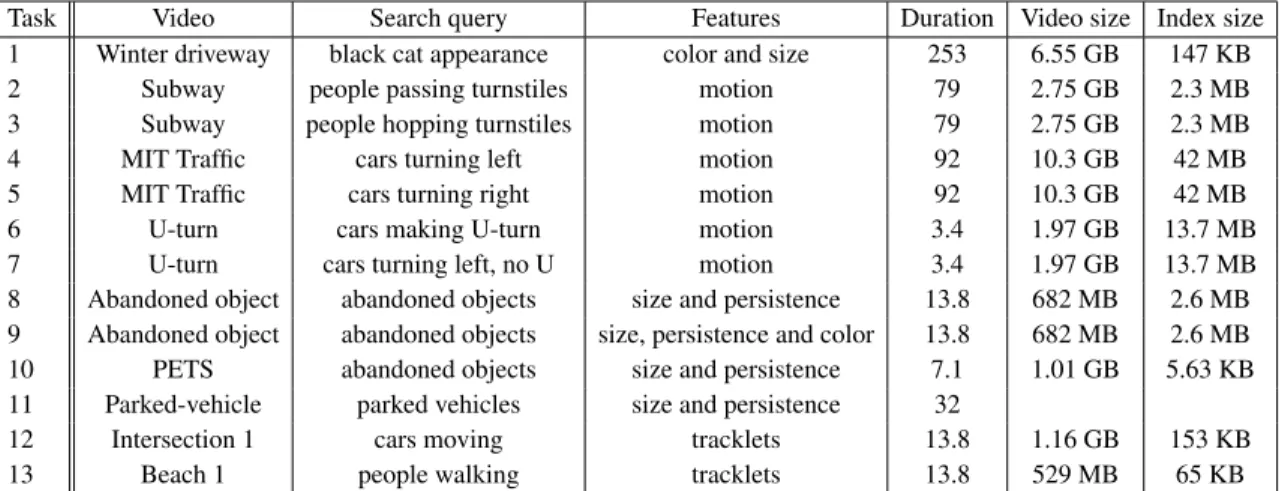
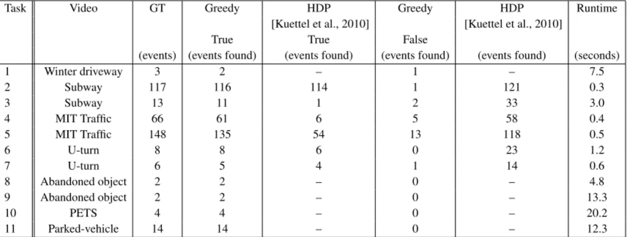
3.1 Tasks’ number, videos, search query, associate features, video duration (min.), video size and index size. Videos of Task 12 and 13 have a frame rate of 2 frames per second. Tasks 1, 8, 9, 10, 11, 12 and 13 use compound search operators. The index size can be several orders of magnitude smaller than raw video. Our use of primitive local features implies that index times and index size are both proportional to the number of foreground objects in the video. Consequently, index size tends to be a good surrogate for indexing times. . . 47 3.2 Results for the elevens tasks using greedy optimization and HDP labels.
Crossed-out rows correspond to queries for which there was no correspond-ing topic in the HDP search. Third row contains ground truth (GT). . . 50
4.1 The run times for baseline [Casta˜n´on and Caron, 2012], brute force and DP algorithms on the VIRAT (top) and YUMA (bottom) datasets. When a brute force algorithm is infeasible, we estimate run-time based on a sub-set of solutions. . . 78
1·1 Whether for identifying people in a crowd or figuring out what’s worth looking at in surveillance footage, video search is a necessary part of many large video systems. . . 2
3·1 Top: Examples of CCTV footage. Bottom: Example of Airborne footage. Blue and green boxes show zoomed-on regions. Objects of interests (cars in this figure) usually have much lower contrast in Airborne footage (see red boxes) over CCTV footage. This makes processing Airborne footage more challenging than CCTV. . . 19 3·2 Our video search framework. As data streams in features are extracted and
inserted into a lightweight index. The user defines query of interest and par-tial matches are generated through inverted lookup index. Parpar-tial matches are then combined into full matches by means of Dynamic Programing. The final output is a video segment matching the user query. . . 22 3·3 (Left) A video of sizeW×H×F divided intoDocumentst. Eachdocument
contains non-overlappingAframes, and each frame is divided into tiles of sizeB×B. Temporal aggregation of tiles overAframes generate anatom. (Right) Tree structure of atoms. Here every set of four adjacent atoms are linked to the same parent. This forms a set of partially overlapping trees. . 23
low) moving near a junction, (c) Frame subtraction and (d) result after ap-plying morphological opening. The final result (d) is void of noisy data shown in red in (c). Second row, from left: Two frames showing a group of people (shown in yellow) walking near a beach, (g) detection after applying morphological opening and (h) detected candidates of size more than 150 pixels in green. . . 27 3·5 Examples of tracklets generated by the technique discussed in Sec. 3.3.3.
Here tracks start with a red cross and their tails have different color. The example of the left shows tracklets generated for cars while the example on the right shows tracklet generated for a group of people walking on the beach. 29 3·6 Motion features (in red) of four buckets of a hash table. Arrow sizes are
proportional to the number of hits at the corresponding sites. Here the four buckets describe: (a) side walk (b) upper side of the street (c) lower side of the street (d) crosswalk. . . 33 3·7 A GUI for creating queries with instructions outlined from 1-5 (see red
regions). Here the user draws queries of interest (in blue) and selects addi-tional target properties (see step 3,4). . . 35 3·8 Searching for a U-turn. Despite three sequences of actions have same
RQ,τ(∆)values (see Seq. 1,2,3), yet only Seq.3 contains a valid U-turn. . . 39
3·9 Example of the V matrix. The query is actions A, C, A, T, and the seven documents in the video corpus each contains a single action, T, A, A, C, A, G, T. The values forWI, WD, WC andWM are−1,−2,1and3in this
example. The optimal path, A,A,C,A,G,T, involves an insertion, a contin-uation and a deletion. It is found by tracing backwards from the maximal element, valued at 11. . . 43
arrows), ROI (shown in green) and the generated retrieval (bottom to query, in red rectangle). Here red dots are trees whose profile fit the query. . . 44 3·11 Examples of the examined routes. Routes are shown in yellow/red arrows
and they start from point X and end at point Y. Some of the routes undergo strong occlusion (see dashed yellow region, top row, first column, for route in second column) and others undergo many turns (see first row, second and last column). . . 45 3·12 ROC curves for the U-turn, subway and MIT traffic datasets. Our methods
significantly out-perform HDP [Xiang and Gong, 2008, Kuettel et al., 2010]. 48 3·13 ROC curves for cars and humans in airborne data. . . 53
4·1 In the archival step, we take in incoming data, extract attributes and rela-tionships and store them in hash tables. In the query creation step, a user utilizes our GUI to create a query graph that is used to extract the coarse graph C from archive data. In the Maximally Discriminative Subgraph Matching (MDSM) step, we calculate the maximally discriminative span-ning tree (MDST) T∗ from the query graph, retrieve matches to it, and assemble them into ranked search results for the user. . . 59 4·2 (Left) Given a video, we extract (Right) Atoms are grouped into two-level
trees - every adjacent set of four atoms is aggregated into a parent, forming a set of partially overlapping trees. . . 61 4·3 The graphical representation of an “object deposit” event. . . 64 4·4 The graphical representation of a “meeting” event. . . 65 4·5 The probabilities associated with 5 of the attributes in the VIRAT dataset.
Being an object, as opposed to a car or a person, is the most unlikely at-tribute and thus the most discriminative. . . 69
nificant elevation, leaving few pixels on targets as small as people or vehicles. 77 4·7 Precision/recall curves for the meeting activities in the VIRAT video dataset.
Note that we optain perfect precision/recall for both brute force and dy-namic programming approaches. . . 78 4·8 Precision/recall curves for the object deposit, object removal, mount and
dismount activities in the VIRAT Ground Dataset. We show baseline [Casta˜n´on and Caron, 2012] search results in green, MDSM results in red, and brute force results in blue when they diverge from MDSM results. . . 79 4·9 Precision/recall curves for u-turn, suspicious stop, mount and dismount
ac-tivities in the YUMA dataset. We show baseline [Casta˜n´on and Caron, 2012] search results in green, unfiltered MDSM results in red, and brute force results in blue. . . 80
5·1 Given a query graph, our goal is to find the set of matchings in the archive graph above a particular score threshold. . . 88 5·2 Given a query, sliding window search space reduction creates a window,
shown in purple, and slides it through the space, creating a filtered archive graph containing only nodes and edges within the window. . . 89 5·3 Node/Edge filters remove nodes and edges from the archive graph which
could not independently match any nodes or edges in the query graph. . . . 90 5·4 In (a), we select a minimum spanning tree ofQto be our query treeT. In
(b), we solve for all matches to T in the archive graph and remove nodes not present in a matching. . . 91
we extract features for object detection and tracking. We store the resulting detections and associations in a database. When a queryQis created by a user through our GUI, we downsample the data to create a filtered graph
A0. We iteratively reduce the filtered graph through matching using our successive search space refinement algorithm, then solve a small subgraph ranking problem to produce results. . . 96 5·6 The average number of nodes remaining after each iteration for the baseline
(green) and successive-search space reduction (red) approaches on archive graphs of size 500, 1000 and 3000. In the first row,pconn =.25and|Fv|=
20. In the second rowpconn=.5and|Fv|= 30. . . 100
5·7 Precision/Recall curves for the Object Deposit, Object Takeout, Mount and Dismount activities in the VIRAT dataset. Recursive search space reduc-tion is shown in red, with a baseline approach based on space-time feature accumulation shown in green. In these experiments, ground truth was used for detection and track information. . . 101 5·8 Precision/Recall curves for the Object Deposit, Object Takeout, Mount and
Dismount activities in the VIRAT dataset. Recursive search space reduc-tion is shown in red, with a baseline approach based on space-time feature accumulation shown in green. We track aggregate channel features [Dollar et al., 2014] using [Andriyenko et al., 2012] in these experiments. . . 101 5·9 This figure highlights some of the issues involved in tracking and detection
in surveillance scenarios. In (a), the algorithm misses a pair of people talking in the shadow of a building. In (b), two people talking are mis-classified as a single person. In (c), a person comes too near a car, enters its shadow, and is not detected. . . 102
ARG . . . Attributed Relational Graph BP . . . Belief Propagation
CCTV . . . Closed Circuit Television DP . . . Dynamic Programming GMM . . . Gaussian Mixture Model GT . . . Ground Truth
GUI . . . Graphical User Interface HDP . . . Hierarchical Dirichlet Process HMM . . . Hidden Markov Model
HOG . . . Histogram of Oriented Gradients KLT . . . Kanade - Lucas - Tomasi
LSH . . . Locality-Sensitive Hashing
MDSM . . . Maximally Discriminative Subgraph Matching MDST . . . Maximally Discriminative Spanning Tree MIT . . . Massachusetts Institute of Technology MST . . . Minimum Spanning Tree
N P-Hard . . . Non-deterministic Polynomial time hard UAV . . . Unmanned Aerial Vehicle
ROC . . . Receiver Operating Characteristic ROI . . . Region of Interest
ST-AOG . . . Spatio-Temporal And/Or Graph STIP . . . Spatio-Temporal Interest Points
Chapter 1
Introduction
1.1
Introduction
As cameras become cheaper and more ubiquitous, algorithms that reason over large video corpora are becoming increasingly vital. Faced with an overwhelming amount of infor-mation, users seek answers to both specific (‘What’s moving?’) and abstract (‘What’s important?’) questions about video. With nearly 1 billion hours of video on a single web-site like youtube, a web browser might be interested in automatically generating tags for video [Siersdorfer et al., 2009, Wang et al., 2012] to allow easier browsing. In retail, a security guard looking at a dozen monitors might want an algorithm to tell him what’s moving [Barnich and Van Droogenbroeck, 2011, Chen et al., 2012], or what’s unusual [Li et al., 2014]. A person browsing through family videos might be interested in finding all instances of a certain person [Li et al., 2002], a particular activity like running or jump-ing [Oneata et al., 2013, Sadanand and Corso, 2012]. A law enforcement officer presented with a wealth of street surveillance might be interested in higher-level activities, such as who is jaywalking, running a red light, or loading objects into a car [Zhu et al., 2013, Kwak et al., 2013, Casta˜n´on et al., 2015].
Of these manifold types of visual reasoning, we are primarily interested in semantic video search: looking for things in a video that have clear semantic meanings. Semantically-meaningful queries differ from concepts like cornerpoint features, textures, and integral images [Mita et al., 2005] because they are easily described by a person. Examples of se-mantic concepts are objects and activities; everybody knows what a basketball or jogging
Figure 1·1:Whether for identifying people in a crowd or figuring out what’s worth looking at in surveillance footage, video search is a necessary part of many large video systems.
should look like, with few exceptions. There are two primary families of algorithms that reason over semantic concepts: classification and search engines.
A classification engine is typically provided with a set of videos of different classes and expected to label each of the videos with the correct class. In images and video, class tends to correspond to the object or activity occuring in the image or video. In many modern datasets [Sch¨uldt et al., 2004, Yao et al., 2011, Blank et al., 2005, Rodriguez et al., 2008, Soomro et al., 2012, Marszałek et al., 2009] this is not a multilabel problem because each video in the corpus has only one correct label. Classification engines can learn their classes from training sets of exemplar videos [Weinland et al., 2007, Laptev et al., 2008, Oneata et al., 2013, Sadanand and Corso, 2012], human input, or a combination of both [Felzenszwalb et al., 2010, Raptis et al., 2012, Raptis and Sigal, 2013, Wang and Mori, 2009, Wang and Mori, 2011]. A classification engine is typically provided with a set of videos of different classes and expected to label each of the videos with the correct class. In images and video, class tends to correspond to the object or activity occuring in the image or video. In many modern datasets [Sch¨uldt et al., 2004,Yao et al., 2011,Blank et al., 2005, Rodriguez et al., 2008, Soomro et al., 2012, Marszałek et al., 2009] this is not a multilabel problem because each video in the corpus has only one correct label. Classification engines can learn their classes from training sets of exemplar videos [Weinland et al., 2007, Laptev
et al., 2008,Oneata et al., 2013,Sadanand and Corso, 2012], human input, or a combination of both [Felzenszwalb et al., 2010, Raptis et al., 2012, Raptis and Sigal, 2013, Wang and Mori, 2009, Wang and Mori, 2011].
Once a classifier is trained, it can be applied in parallel to each video in a corpus. While training time can be prohibitive, in a real-world scenario, model training happens offline. Thus, the primary challenge of classification problems is to learn a model of sufficient fidelity to differentiate between the classes it trains on.
In contrast, search engines operate in two modalities. First comes the archival modality, where the engine is presented with the video corpus and has to assemble it in a format to be reasoned over quickly. Second is the search modality, where the search engine is provided a query activity or object and has to identify all locations in the video corpus where that query occurs.
Challenges of search include:
• Data lifetime: since video is constantly streamed, there is a perpetual renewal of video data. This calls for a model that can be updated incrementally as video data is made available, as well as one which scales well with the temporal extent of the video.
• Unpredictable queries: the nature of queries depends on the field of view of the camera, the scene itself and the type of events being observed. The system should support queries of different nature, such as identifying abandoned objects and finding instances of cars performing U-turns.
• Unpredictable event duration: events in video are ill-structured. Events start at any moment, vary in length and overlap with other events. The system is nonetheless expected to return complete events whatever their duration may be and regardless of whether other events occur simultaneously.
• Clutter and occlusions: urban scenes are subject to high number of occlusions. Tracking and tagging objects in video is still a challenge, especially when real-time performance is required.
1.1.1 Representation and Models
Of course, efficient representation of large video corpora has been studied in other parts of the computer vision community. Videos and images contain a tremendous amount of re-dundant information, a fact exploited in both image [Taubman and Marcellin, 2012, Taub-man, 2000] and video [Le Gall, 1991] compression. Since the earliest days of computer vision, approaches [Lowe, 1999, Li et al., 2002, Efros and Berg, 2003] have tried to find ways to capture the minimum essential information required from a video to accomplish a particular task. Many relevant approaches are compared in [Mikolajczyk and Schmid, 2005] for the purposes of local interest region detection. Of these, the Scale-Invariant Fea-ture Transform [Lowe, 1999], a descriptor of interest points in images, was the earliest popular feature for representing objects in videos. Another popular feature is Haar-like features [Mita et al., 2005, Zhang and Viola, 2008], based on wavelets, that were used extensively in face detection [Viola and Jones, 2004].
Moving from images to videos introduces time as a third dimension. Videos tend to contain more redundant information than images, as an immobile background (with un-changing recording conditions) yields the same set of pixels at every point in time. Thus, video feature description tends to focus on areas of motion, with the assumption that the things of interest in video move. Some approaches [Scovanner et al., 2007] directly ex-tend the SIFT framework, while others extract pyramids of integral images [Dollar et al., 2014, Doll´ar et al., 2009] to classify local patches.
Acquiring these models for video corpora has been the subject of much research over the last 30 years. Exemplar-based approaches [Tianmin Shu et al., 2015, C¸ eliktutan et al., 2013] are provided sets of training examples for each potential object or activity to be
de-tected in the corpus. However, it has generaly been recognized that the number of training examples cannot match the increasing complexity of classifiers and activities [Ryoo and Aggarwal, 2010, Kwak et al., 2013].
In the face of increased query complexity, user-driven queries have become a popular way to access more complex models. Early works [Chang et al., 1998, Zhong and Chang, 1999] focused on enabling users to draw simple motions, while later approaches [Hu et al., 2013] allowed sketches for object detection in videos.
These approaches present a good-starting point for a system which aims to efficiently represent large video corpora for fast search. Most of these features have reached the point where they can be reasonably extracted in real-time from streaming video, and their memory footprint is far less than that of the raw video itself.
1.1.2 Classification and Detection
In the search problem, we ask a system to find all the examples of a particular query. For certain datasets [Yao et al., 2011, Soomro et al., 2012, Sch¨uldt et al., 2004, Marszałek et al., 2009, Blank et al., 2005, Rodriguez et al., 2008], where each element of the corpus (video or image) contains exactly one object or activity, such as jumping rope or running, search can be a specialization of object or activity classification. Ample work has been done building video models and distance metrics between them, to answer the question ‘Do these contain the same thing?’. The earliest of these models are histogram models [Laptev et al., 2008, Oneata et al., 2013, Sadanand and Corso, 2012], which accumulate local features into a histogrammed representation of the video in question and use statistical distance measures like earth-mover’s distance [Rubner et al., 2000] to compare distributions. Other approaches track spatio-temporal interest points through the video and compare trajectories [Ikizler and Forsyth, 2008,Wang et al., 2013,Wang and Schmid, 2013,Zhang et al., 2014a]. Dense trajectory approaches measure local optical flow and directly compare motion via correlation, but tend to be too computationally expensive to perform on large video corpora
in real time.
Given our stated desire to scale well with the archive video corpus size, we are par-ticularly interested in graphical models of activity. These models were originally used to search for objects in images [Felzenszwalb et al., 2010, Tianmin Shu et al., 2015]. Each image was represented with an attributed, relational graph (ARG), with each node repre-senting a local feature, and each edge encoding the spatial relationship between nodes. In classification, images are compared via graph matching [Riesen and Bunke, 2009, Berretti et al., 2007, Cho et al., 2010], which produces an assignment of nodes from one image’s graph to the other’s. The distance metric for this association typically takes the form of a sum of kernel functions between matched node and edge pairs.
Graphical representations of video have also been popularized for activity retrieval in particular video corpora. Specifically, when each video in a corpus contains a single activ-ity, graph-matching approaches [C¸ eliktutan et al., 2013, Ma et al., 2013] have proven to be effective in comparing activities.
Unfortunately, while in many datasets each element of the corpus has one and only one activity happening, this is not true in some real-world applications. In video surveillance, the corpus can be a single extremely long video. This has lead to a number of efforts within the search community to reduce this problem to classification, where it can be solved easier. In news video or television, the video can be divided into ‘shots’, [Song and Fan, 2006,Sivic and Zisserman, 2003,Sujatha and Mudenagudi, 2011], with each shot having a single topic. However, for generic video corpora without a-priori knowledge, there has only proven to be a single reliable way to perform pattern recognition for search: to run a sliding window across each video.
Sliding window approaches are an extremely popular way to transform a search prob-lem into a classification probprob-lem, and they see extensive use in both object [Viola and Jones, 2001, Philbin et al., 2007, Sivic and Zisserman, 2003, Johnson et al., 2015] and activity
de-tection [Gaur et al., 2011, Lin et al., 2014]. If a query has a maximum size in space-time, a sliding window approach will attempt to segment a video into overlapping space-time boxes of that size, and independently classify each of the boxes.
In certain circumstances, applying sliding windows over every video in a corpus to detect activities can be effective. In movies or youtube videos with narrow field of view, an activity can be expected to take up the whole view, so the sliding window only has to slide over time. Likewise, those videos are more likely to contain only one thing going on within any window because of the limited view.
In more generic video modalities, particularly surveillance video [Oh et al., 2011, Fer-ryman, 2006], the assumptions that enable effective sliding window search fall apart. First, surveillance video corpora are extremely large, rendering a sweeping approach unappeal-ing. Second, the amount of background activity is generally far larger than the activity that matches the query. Finally, the maximum size of a query often spans a significant amount of space and time, so any given window that contains the query activity also likely contains a significant amount of background activity.
Subgraph matching has been used in a diverse array of fields to identify sub-structures of larger graphs. Sub-graph and graph matching are also commonly used in image search applications [Christmas et al., 1995,De la Torre, 2012] as well as image duplicate detection [Zhang and Chang, 2004]. In image search and image duplicate detection, the goal is the same: to match the graph extracted from a query image to the graphs extracted from each image in a corpus. Subgraph matching is used to allow these algorithms to be robust to small amounts of clutter. These problems differ significantly from ours - because the corpus is divisible into a series of relatively small graphs, one for each image, it can be solved efficiently by a series of subgraph matching problems.
In our problem, we are looking at an extremely asymmetric subgraph matching problem with a dense archive graph containing millions of nodes and a query graph containing up
to a dozen nodes. Algorithms for subgraph matching in this context are more often used in bioinformatics [Bonnici et al., 2013,Sun et al., 2012,Zhang et al., 2010,Koutra et al., 2011], a field where query graphs generally represent proteins or amino acids to be searched for in a larger dataset. Because subgraph matching is provably N P-hard [Ullmann, 1976], efficient algorithms [Sun et al., 2012, Zhang et al., 2010] focus on search space reduction before actually solving the subgraph matching problem.
1.1.3 Overview and Notation
A video search system operates in two modalities: archival and search. During the archival step, we process each video in a video corpus and extract features from a pre-defined feature vocabulary Fv. These features are all local - they are associated with a certain area or
location in space/time in a specific video. We store these locations in an inverted index by feature and feature value. So, if the system needs to find all places in a video corpus where we found the color ‘red’, it would go to the color index and look in the ‘red’ bin, which would contain all location/video pairs where that color was found.
In our later systems in Chapters 4 and 5, we also focus on the relationships between these features. For each pair of locations that might potentially satisfy a relationship in our relationship vocabulary Fe, we check to see if that relationship exists. If so, we hash the
pair of locations that satisfy the relationship to an inverted index based on the relationship they satisfy. As an example, in the ‘same as’ bin, we would have all pairs of locations where we believe the same object is at both locations.
At the end of our archival step, we have a bunch of indices, some for local features and some for relationships between them. These indices implicitly represent an archive graph
A =G(V(A), E(A)). In this graph, each nodev ∈V(A)is the collection of features at a specific spatiotemporal location in a given video of the corpus. An edgee ∈ E(A)exists between two nodes if a relationship has been found between them.
cor-pus. He assembles features into nodes (‘a large, red, moving object’) and then adds edges containing relationships. The result is the query graphQ=G(V(Q), E(Q). In search, our goal is to find the set of subgraphs ofAwhich best match the query graphQ. Alternately, our goal is to find a set of matchingsMwherem∈ M :V(Q)→V(A).
We rank these matchings according to a score function S(m, Q, A) which incorpo-rates distances between nodesdv(va, vi), distances between edgesde((va, vb),(vi, vj)), and
also penalties for failing to find a matching for an edge entirely. Finally, we return in de-scending order the clipped video segments corresponding to the set of matchings for which
S(m, Q, A)is larger than thresholdτ.
1.1.4 Our Contributions
In this dissertation, we describe a functional system that can process and archive large video corpora in real-time. Later, when provided a query by a user, our system is able to find and rank matches to the query in a matter of seconds and display these results. The novel components of this system are:
1. Inverted indices for efficient archive downsampling.In Chapter 3 we introduce an inverted hashing scheme for simple features. In 4, we use these and other indexing techniques to dramatically downsample a video corpus to the set of features that are potentially relevant to a given query. This allows us to efficiently reason over large video corpora without prior knowledge and without that each corpus being subdivided into small videos.
2. Sub-graph matching in video search.In Chapter 3, we introduce temporal relation-ships on simple features to find a wide variety of user-driven queries using a novel dynamic programming approach. In Chapter 4, we expand this approach to include spatial relationships and search for arbitrary graphs in large videos. In particular, we use a subgraph matching approach to render our method agnostic to background
noise. Other approaches use bipartite matching [Lin et al., 2014] or require a tree-based query [Tianmin Shu et al., 2015], and are thus unable to represent activities with a similar degree of structural complexity.
3. Tree-matching for space-downsampling in video search. We introduce a novel method for successive search-space reduction based on selecting the Maximally Dis-criminative Spanning Tree in Chapter 4. In Chapter 5, we extend this method to iteratively reduce the search space based on the statistics of the dataset. This ap-proach significantly outperforms contemporary algorithms for search space reduction in subgraph matching like random trees.
Chapter 2
Related Work
In this work, we propose a fully operational video surveillance system that utilizes a number of pre-existing approaches, as well as comparing to others. While we cite these works directly, for purposes of clarity we explain the most important of them in this chapter.
2.1
Locality Sensitive Hashing
In order to be able to quickly return a set of matches to a given search, we hash features to inverted indices. Features like object type, are hashed via regular hash tables because there is no notion of distance between types. However, for continuous features like motion direction, object size, and persistence or activity, we use Locality-Sensitive Hashing [Datar et al., 2004] (LSH) such that a query to the inverted index returns (with high probability) all locations that have a feature within radius r of the query. This has the advantage of mitigating, to some extent, user and feature extraction errors that cause a mismatch between what the user expects and what is stored in the archive.
For our implementation of Locality Sensitive Hashing, we have three parameters: col-lision radius r, dimensionality of the feature data dand number of tablesN. Our goal is to choose a set of hash functionsH1, ..., HN whereHi :Rd →Z. Following the approach
in [Datar et al., 2004], we use Algorithm 1.
This createsN hash functions for a given feature type, like color, with dimensionality
d. As video is processed, we get measurements of features, paired with spatiotemporal locations ({x, y, t} for video). For example, we might see the color red in the first frame
Algorithm 1LSH Function Creation
1: procedureCREATE LSH FUNCTIONS(r, d, N)
2: for alli∈ {1, ..., N}do .For each table
3: Draw each element ofa∼N(0,1) .Each element ofais drawn from a univariate normal distribution
4: Drawb ∼unif(0, r) .The offsetbis drawn uniformly from the range[0, r]
5: Hi(x)← ba·xr+bc
6: end for
7: end procedure
in the upper-left hand corner. For each of ourN hash functions, we computeHi(red), and
store the spatiotemporal location in that bin.
When somebody asks for all locations with a color, like purple, we computeHi(purple)
for each of our hash functions, and look at the contents of thoseN bins. If a given location appears in more than τcolor percent of the bins, we consider that location to contain the
color purple.
We independently create sets of hash tables for each feature type in a dataset.
2.2
Smith-Waterman Algorithm
Some of our work in Chapter 3 extends the Smith-Waterman algorithm for dynamic pro-gramming. This algorithm takes in two strings of characters and attempts to compute the match that is minimally distorted. The model for distortion is that the string inais present in b, except that characters in a may be missing (“deletion”), and that in the middle of an otherwise perfectly good match there may be extraneous characters in b (“insertion”). We are given fixed penalties wk and wl for insertion and deletion, respectively. Second,
between each elementai ∈aandbj ∈jis a scores(i, j)indicating how well they match.
Given these quantities, our goal is to pick a starting point t wherea0 maps to bt, and
an optimal series of insertions and deletions to maximize the sum of the matching scores minus the penalties. To achieve this, Smith and Waterman set up a matrixH ∈n×m, as
follows:
H(i,0) = 0 ∀i= 1...n (2.1)
H(0, j) = 0 ∀j = 1...m (2.2)
H(i, j) = max(0, H(i−1, j−1) +s(ai, bj), H(i−1, j) +wk, H(i, j−1) +wl)
(2.3)
Most importantly, when calculating this matrix, the Smith-Waterman algorithm keeps a pointer to which of the four options (representing a new start, an element happening correctly, a deletion or an insertion) were chosen at each elementH(i, j).
To compute the optimal match, we use backtracking. The Smith-Waterman algorithm selects the maximum element ofHand then iteratively asks “Which element generated the maximum value that we used?”. This backtracking process produces a series of matches, insertions and deletions corresponding to the optimal match.
2.3
Sliding Window Approaches
A number of approaches [Lin et al., 2014,Tianmin Shu et al., 2015] utilize sliding windows to reduce the space over which they have to search. In [Lin et al., 2014], the goal is to match a textual description of an activity to the KITTI [Geiger et al., 2012] dataset. This dataset contains recordings of a Volkswagon-mounted camera driving around Karlsruhe, Germany. In [Lin et al., 2014], a small subset of this dataset is used: 21 30-second video clips are used - 13 for training their set of concepts, and eight as a search corpus. The selection of eight short videos as a search corpus can be viewed as a specialization of a 30-second sliding window. A complete sliding window approach for queries with 30 30-second maximum length would be to take every time interval[t0, t0 + 30]in the video corpus and
complexity, [Lin et al., 2014] elect to only look at eight such videos.
For each video, they solve a bipartite matching problem. Given a textual query like “A car is moving forwards”, they convert it to a set of featuresu∈U, and have a set of features
v ∈V for each video segment. They compute a matching scorehuvbetween featureuand
featurev based on appearance and motion, and compute a global assignment scoreSyand assignment vectory∈ {0,1}U×V: S(y) = X uv huvyuv (2.4) max y S(y) (2.5)
subject to the constraints thatyassign each element ofU to one or less elements ofV. Videos are ranked for the user in descending order of their global assignment score.
Compared to our approach, this method does not take advantage of relationships be-tween features - it is looking to find a single optimal match for every feature in the query. However, common to a lot of sliding window approaches, by using a relatively small slid-ing window in time (30 seconds), they do implicitly enforce that all the features must occur within 30 seconds of one another, which is a sort of relationship. When features alone are sufficient to differentiate the activity in question, and the activity has limited spatiotemporal extent, this approach can be effective.
[Tianmin Shu et al., 2015] use a similar approach to dividing an aerial events dataset. Using combinations of ground truth, tracks, and manual object annotations, they partition tracks into non-overlapping sets. For each event, they have learned a spatio-temporal and/or graph (ST-AOG) that is a series of trees (in space) linearly sequenced in time. For each partitioned set of tracks, they slide a window of length T, and at each window solve a dynamic programming problem that assigns detections in the tracks present in that window to elements of the graph. Videos are classified as the event that has the best match within
their windows.
This method does take into account relationships between features. However, the ac-ceptable structure for an input is limited to trees because of the necessity of solving via dynamic programming. Further, it assumes that moving objects within the data can be clearly partitioned into disjoint sets. In more realistic surveillance datasets, this is not the case - objects are continually moving.
In this work we aim to produce a system that takes in arbitrary graphs (expressed by our vocabulary) and makes few assumptions about the video corpora that we are searching over. We do not assume that the dataset is partitionable, nor that our input graph has any particular structure. Unlike the above approaches, we also do not learn models from exemplar video. In our work, we compare to a feature-accumulation approach like [Lin et al., 2014] to show the utility of incorporating relationships between features, and to a sliding window approach later. In our experiments, we merge spatiotemporally overlapping windows when appropriate to attain video intervals for users.
Dynamic Programming for Activity Search
In this chapter, we present a content-based retrieval method for long surveillance videos both for wide-area (Airborne) as well as near-field imagery (CCTV). Our goal is to re-trieve video segments, with a focus on detecting objects moving on routes, that match user-defined events of interest. The sheer size and remote locations where surveillance videos are acquired, necessitates highly compressed representations that are also meaningful for supporting user-defined queries. To address these challenges, we archive long-surveillance video through lightweight processing based on low-level local spatio-temporal extraction of motion and object features. These are then hashed into an inverted index using locality-sensitive hashing (LSH). This local approach allows for query flexibility as well as leads to significant gains in compression. Our second task is to extract partial matches to the user-created query and assembles them into full matches using Dynamic Programming (DP). DP exploits causality to assemble the indexed low level features into a video segment which matches the query route. We examine CCTV and Airborne footage, whose low contrast makes motion extraction more difficult. We generate robust motion estimates for Airborne data using a tracklets generation algorithm while we use Horn and Schunck approach to generate motion estimates for CCTV. Our approach handles long routes, low contrasts and occlusion. We derive bounds on the rate of false positives and demonstrate the effective-ness of the approach for counting objects, motion pattern recognition and abandoned object applications.
3.1
Introduction
Video surveillance camera networks are increasingly common, generating thousands of hours of archived video every day. This data is rarely processed in real-time and primarily used for scene investigation purposes to gather evidence after events take place. In military applications UAVs produce terabytes of wide area imagery in real-time at remote/hostile locations. Both of these cases necessitate maintaining highly compressed searchable rep-resentations that are local to the user but yet sufficiently informative and flexible to handle a wide range of queries. While compression is in general lossy from the perspective of video reconstruction it is actually desirable from the perspective of search since it not only reduces the search space but it also leverages the fact that for a specific query most data is irrelevant and pre-processing procedures such as video summarization is often unnecessary and inefficient. Consequently, we need techniques that are memory and run-time efficient to scale with large data sets, and be able to retrieve video segments matching user defined queries with robustness to common problems, such as low frame-rate, low contrast and occlusion.
Some of the main challenges of this problem are:
1.) Data lifetime: The model must scale with the growing size of video data.
The continuous stream of video data requires a model that can handle this growing temporal size. This requires periodic processing of the new data as it streams in the system.
2.) Unpredictable events:
Some events are rare, yet they could be of great interest. For instance a person dropping a bag and continuing walking, or a car violating a traffic light are examples of not so common events. Yet their detection is valuable as it could help in forcing the law and preventing terrorist attacks. The system should be able to support such events.
3.) Clutter and Low Contrast:
processing temporal queries. Low contrast is common in airborne footage while clutter is frequent in videos of urban areas.
4.) Unpredictable event duration:
Events vary in duration, co-occur with each other and could start and end anytime. Accurate estimation of an event time window is important. Such task is made more difficult in regions of high clutter and poor contrast.
This chapter extends our method for content-based retrieval [Casta˜n´on and Caron, 2012] to the domain of airborne surveillance. In [Casta˜n´on and Caron, 2012] we pre-sented a query-driven approach where the user draws routes manually. The algorithm then retrieves video segments containing objects that moved in the user supplied routes. Our technique consists of two steps: The first extracts low level features and hashes them into an inverted index using locality-sensitive hashing (LSH). The second stage extracts partial matches and assembles them into full matches using Dynamic Programming (DP).
While [Casta˜n´on and Caron, 2012] dealt with CCTV data, in this chapter we handle motion patterns in aerial view images shot from a UAV (airborne data). Handling such data is more challenging than handling CCTV due to their lower frame rate and lower contrast (see Fig. 3·1 ). As a result certain features such as optical flow information (extracted using Horn and Schunck technique [Horn and Schunck, 1981]) are rendered highly noisy. Hence for airborne data we first generate tracklets, using ideas from [Piti´e et al., 2005, Baugh and Kokaram, 2010], and then generate motion estimates from those tracklets. We use these motion estimates in combination with our previous two-step process to retrieve routes generated by different objects (such as cars and human) while handling long routes, low-contrast, occlusion, and outperforming current techniques.
This algorithm extends our preliminary work in [Casta˜n´on and Caron, 2012] to videos collected via airborne surveillance. Airborne video differs significantly from standard surveillance video: the resolution and contrast of objects of interest is extremely low, and
(a)
(b)
Figure 3·1: Top: Examples of CCTV footage. Bottom: Example of Air-borne footage. Blue and green boxes show zoomed-on regions. Objects of interests (cars in this figure) usually have much lower contrast in Air-borne footage (see red boxes) over CCTV footage. This makes processing Airborne footage more challenging than CCTV.
the frame-rate is extremely low. This poses a number of problems to our standard approach - due to low frame-rate, objects are effectively obscured for significant periods of an ac-tion, as the camera is not taking a picture. Likewise, low resoluac-tion, low contrast and low frame rate make estimation of optical flow unstable. To address these issues, we perform significant filtering work on the raw video both to identify targets and suppress camera artifacts. We also develop a rudimentary tracker which operates effectively in harsh condi-tions. We use the results of this tracker to create a low-level feature set for exploitation by the approach described in [Casta˜n´on and Caron, 2012]. Note that we are not interested in obtaining long-term (i.e. perfect) tracks; instead we are interested in tracklets that are good enough for our retrieval problem.
Our approach differs significantly from current approaches [Kuettel et al., 2010, Xi-ang and Gong, 2008]. In this chapter we assume that there is no prior knowledge on the queries and hence we first extract a full set of low-level features. In addition unlike scene understanding techniques [Kuettel et al., 2010, Xiang and Gong, 2008], we do not incorpo-rate a training step as this would scale unfavorably with the magnitude of the video corpus. Instead, our technique exploits temporal orders on simple features, which in turn allows ex-amining arbitrary queries and maintains a low false rate. We show significant improvement over scene-understanding methods [Kuettel et al., 2010], both in terms of search accuracy and computational complexity. We also show how tracklets are better suited for airborne footage than optical flow. Results for CCTV data are also included.
3.2
Overview
Our procedure consists of two main stages. The first reduces the problem to the exam-ined data while the second reasons over that data. Fig. 3·2 shows this procedure in more detail. Low level features are continuously extracted as data streams in. Here features as activity, object size, color, persistence and motion are used. For CCTV footage motion is
estimated using the Horn and Shunck approach [Horn and Schunck, 1981], while for Air-borne footage motion is estimated using tracklets. LSH [Gionis et al., 1999] is then used to hash the extracted low level features into a fuzzy, light-weight lookup table. LSH reduces the spatial variability of examined features and reduces the queries search space into a set ofpartial (local) matches.
The second step of our search algorithm optimizes over the partial matches in order to generate full matches. Here video segments of partial matches are combined to fit the examined query. Our search approach simplifies the problem from examining the entire video corpus into reasoning over the partial matches that are relevant to our query. This feature is advantageous especially in examining surveillance videos where hours of video may not be of interest to an observer. Hence our approach reduces the search workload considerably.
We examine two approaches for generating full matches. The first is a greedy approach based on exhaustive examination of partial matches. The second approach exploits tem-poral ordering of component actions. Here Dynamic Programming (DP) processes partial matches and finds the optimal full match for a given query. We present two DP versions, one that uses optical-flow (for CCTV) and another that uses tracklets (for Airborne). Our technique outperforms current approaches and we show that increased action complexity drives false positives to zero.
3.3
Feature extraction
In this section we explain how to extract relatively basic features. In our previous work [Casta˜n´on and Caron, 2012], we observe that the retrieval process is not strongly feature dependent, and use coarse features both for the purposes of robustness and speed of com-putation to address problems of data lifetime. For purposes of completeness, we present that extraction process in Section 3.3.2.
Features User Commands Query Creation Feature Extraction Lightweight Index Inverted Index Lookup Dynamic Programming LSH Index
Set of Query Features Partial
Matches
Video Segments
Figure 3·2: Our video search framework. As data streams in features are extracted and inserted into a lightweight index. The user defines query of interest and partial matches are generated through inverted lookup index. Partial matches are then combined into full matches by means of Dynamic Programing. The final output is a video segment matching the user query.
Feature extraction for airborne video is significantly more difficult. As the video is low frame-rate, low-contrast and colorless we focus on motion features. Due to the lack of image quality, histograms of optical flow are inaccurate - as such, we perform short-term tracking and derive motion information based on these tracklets. This process in described in Section 3.3.3.
For our system to work, we need a spatio-temporal structure to summarize local mo-tion features. Although we could use 3D atoms (3D spatio-temporal block of video) as in [Wang et al., 2009], we found empirically that this structure is very sensitive to slight vari-ations in the dynamics and shape of moving objects. For example, a car running through a 3D atom would leave a different signature than if it were slightly shifted and went through half that atom and half a neighboring atom. Instead, we use a hierarchical structure which aggregates information from neighboring atoms. This structure is described in the follow-ing section.
3.3.1 Structure
In this chapter, we treat a video as a spatiotemporal volume of size H ×W ×F where
H×W is the pixel image size and F denotes the total frames in the video. The video is temporally partitioned into consecutivedocuments containingA frames. We illustrate in Fig. 3·3 how to tile a given frame of video usingB×Bsquares of pixels. We formatoms
by amalgamating consecutive tiles overAframes. Depending on video size and frame rate, for CCTV we chose B to be 8 or 16 pixels and A to be 15 or 30 frames. For Airborne footage however we usedB = 20 andA = 1. A much smaller value of A is used here to capture the fine-detailed nature of tracklets. As video is streaming, we extract features in real-time, assigning a set of features (see Sec. 3.3.2 and Sec. 3.3.3) to each atom n to describe its content.
10
14
11
1
2
3
1
Figure 3·3: (Left) A video of size W ×H ×F divided intoDocuments
t. Each document contains non-overlapping A frames, and each frame is divided into tiles of size B × B. Temporal aggregation of tiles over A
frames generate an atom. (Right) Tree structure of atoms. Here every set of four adjacent atoms are linked to the same parent. This forms a set of partially overlapping trees.
de-tected features, we create a spatial pyramid structure. For this implementation, we chose a quaternary pyramid (tree) where each element has 4 children, all spatially adjacent. Be-cause the pyramids overlap, a k-level pyramid containsM = Pk
l=1l
2 nodes, as seen in
Fig. 3·3. Given this formulation, a document withU ×V atoms will be partitioned into
(U −k+ 1)×(V −k+ 1)partially overlapping pyramids for indexing. As an example, we construct a depth-3 pyramid tree in Figure 3·3 to aggregate3×3atoms intoM = 14
nodes.
We compute the feature vector for each node of the tree by an aggregation operator over each of its child nodes. Given node n and its four children a, b, c, d, we formalize aggregation in Eq. (3.3.1).
x(fn)=ψf
x(fa),x(fb),x(fc),x(fd),
whereψf denotes the aggregator over relevant features. The output of this aggregator
is x(fn), a concatenation of all features. Sec. 3.3.2 and Sec. 3.3.3 explain the aggregation process in further detail. For each atom we extract a number of features, so the aggregation of a group ofk×katoms yields{treef}one for feature tree for each featuref. Eachtreef
contains a list ofM feature instances, namelytreef =
n
x(fn)o, because there areM nodes in everyk-level tree.
3.3.2 Feature Extraction for CCTV footage
Existing work [Meessen et al., 2006, Stringa and Regazzoni, 1998, Yang et al., 2009] has shown features such as color, object shape, object motion, and tracks to be effective at the atom level. Because of computational limitations and the constant data renewal inherent to the surveillance problem, we chose to exploit local processing to enable real-time feature extraction. We assume a stable camera (common in surveillance, though an unstable camera could utilize existing stabilization options) and compute a single feature
value for each atom. Note that this feature value does not require any understanding of how many objects are in the atom or what it is composed of - they are a a simple amalgamation of values computed at the pixel level. In our current implementation, we exploit five features:
(1) Activityxa: this feature is associated with moving objects that we detect with a
back-ground subtraction method [Benezeth et al., 2010]. The backback-ground is computed using a temporal median filter over 500 frames of the video and subsequently updated using a running average. For every atom, we compute the proportionxaof pixels that are both not
part of the background and have sufficient motion magnitude. The aggregator is defined as the mean activity of the four children.
(2) Sizexs:In order to detect motion, we create a binary activity mask differentiating
activ-ity from background. We then perform connected component analysis to identify moving objects, with the number of pixels in an object yielding the size. The aggregator for size is the median of the non-zero children, with a default value of zero for all-zero children.
(3) Colorxc:We calculate color by computing a histogram over an atom’s non-background
pixels in 8/4/4 quantized HSL color space. The aggregator is the bin-wise sum of the children’s histograms. Because proportions are important, we do not normalize during this stage.
(4) Persistencexp:The persistence measure identifies objects that are not part of the
back-ground, but stay in one place for some time. To compute it, we accumulate the binary activity mask from background subtraction over time, and measure the percentage of pix-els that have been active for longer than a threshold. Non-background objects which are immobile thus obtain a long persistence measure. The aggregator for persistence is the maximum value among the four children.
(5) Motionxm:In order to compute aggregate motion in an atom, we quantize pixel-level
optical flow, extracted using Horn and Schunck’s method, into 8 cardinal directions. We utilize an extra “idle” bin to denote an absence of significant motion (low magnitude flow),
yielding a 9-bin histogram of motion. The aggregator for motion is the bin-wise sum of the motion histograms for the four children. We note that, like color, we store un-normalized histograms to maintain relative proportion.
We extract all of these features from a real-time streaming video. Upon creation, we assign5descriptors to each atom,{xa, xs,xc, xp,xm}. We assemble an atom’s descriptors
into5feature trees{treea},{trees},{treec},{treep},{treem}, which form the foundation
of the our approach to indexing in Sec. 3.4. After indexing, we discard the feature content; the actual value of the features is implicitly encoded in our lightweight index. Note that the choice for the specific aggregation functions (mean, max, and median) came after empirical validations.
3.3.3 Feature Extraction for Airborne Footage
First, we register airborne images onto a common reference frame. Then, in order to be robust to issues of low contrast and frame rate, we extract tracklets and derive features directly from them. Our tracklet extraction process uses a Viterbi-style algorithm with ideas from Pitie et al. [Piti´e et al., 2005] and Baugh et al. [Baugh and Kokaram, 2010]. At each frame we generate a set of candidates and update existing tracklets with these candidates based on distance in feature and position space.
We are supplied with Airborne footage stabilized with respect to the global camera motion. In order to identify moving objects (cars and people) we use frame differencing. Consecutive frames are used for cars, and frames spaced by 10 for slower-moving humans. We use a very small detection threshold to ensure all false negatives are eliminated. Cars are detected if a frame difference of more than15gray-scale levels is observed. A smaller threshold of10is used for humans detection as they have lower contrast. Some detection errors often occur around borders of trees and objects (see Fig. 3·4, red region). Other artifacts are caused due to local motions as the ones generated by the moving sea waves (see Fig.3·4, blue region). Such artifacts are removed through filtering by size. Here we
(a) (b) (c) (d)
(e) (f) (g) (h)
Figure 3·4: First row, from left: Two consecutive frames showing cars (shown in yellow) moving near a junction, (c) Frame subtraction and (d) result after applying morphological opening. The final result (d) is void of noisy data shown in red in (c). Second row, from left: Two frames showing a group of people (shown in yellow) walking near a beach, (g) detection after applying morphological opening and (h) detected candidates of size more than 150 pixels in green.
first detect connected bodies and remove any body that contains more than150pixels. An example of candidate selection with artifacts removal is shown in Fig.3·4. Note that filtering by size eliminates the vast majority of false alarms. This is evident by examining the blue and red rectangles of Fig. 3·4 before and after filtering (third and fourth columns respectively). Quantitative results show that this filtering reduces false alarms by72.3%and
96.5%for cars and humans respectively. This is taken as the average over processing1000
frames for each of Task 12 and 13 ( see Table 3.1 ). It is worth noting that our algorithm only detects moving vehicles and humans. Stopped vehicles are dealt with by our dynamic programming algorithm which we introduce in Section 3.5.2.
Given a set of detection candidates, our goal is to associate them over time for the purposes of computing tracklets. To do so, we set up and solve a Viterbi Trellis as described
in [Baugh and Kokaram, 2010]. Given a set of detection candidates in framen andn+ 1, we estimate the temporal matching cost of each detection pair:
Cl,m = Λ1kpl−pmk+ Λ2|zl−zm|
+ Λ3f3(sl, sm) + Λ4f4(cl, cm) + Λ5f5(pl, pm). (3.1)
Herelandmdenote the examined candidate of framenandn+1respectively. (p s z c)
are the position, shape, size and color of each examined candidate. Λ1...Λ5 are tunable
weights to emphasize the importance of each term. Position is defined as the geo-registered location, shape is the binary mask of the occupied pixels and size is the number of pixels in the examined mask. The purpose of the five elements of Eq. (3.1) is to ensure that the target: (1) has not moved too far between n and n+ 1, (2) is roughly the same size, (3) the same shape, (4) the same color and (5) it is roughly where we expect it to be given its previous motion and location.
slandsmare binary detection masks for the targets under examination, wheref3(sl, sm)
is the mean absolute error between both masks. Given the color measurements of the examined candidates cl and cm, we fit a Gaussian mixture model (GMM) for cl being
G(cl) [Bouman et al., 1997]. We then estimate f4(cl, cm) as the error of generating cm
from G(cl) [Bouman et al., 1997]. To calculate f5(pl, pm)we first estimate the expected
location oflin the next frame (n+ 1) given its current location in framen. The expected location is estimated using a 3 frame window and a straight line, constant acceleration model. f5(pl, pm)is then taken as the absolute difference between the expected location of
linn+ 1and the actual location ofm.
Given the matching costs for all possible l and m pairs, we approximate the two-dimensional assignment problem by greedy assignment for computational efficiency. That is we match the pairs with least matching cost first, remove them, match the next pair, re-move them and keep doing so until all candidates in framenare matched with candidates
Figure 3·5: Examples of tracklets generated by the technique discussed in Sec. 3.3.3. Here tracks start with a red cross and their tails have different color. The example of the left shows tracklets generated for cars while the example on the right shows tracklet generated for a group of people walking on the beach.
in frame n + 1. Unmatched candidates can begin tracks if we find matches for them in subsequent frames, while tracks which are unmatched for enough frames are terminated. Note that this is a one-to-one assignment process hence no candidate in either framen or
n+ 1 can have more than one match. This assignment, plus efficient computation of f4,
yield a simple tracking approach that can scale to large datasets.
Fig. 3·5 shows examples of tracklets generated by the technique discussed in this sec-tion. Here we show tracklets of cars (see left of Fig. 3·5) and for a group of people walking on the beach (see right of Fig. 3·5). In order to quantitatively evaluate tracklets, we selected the 4 longest streets in our videos and examined every tracklet associated to them. This was equivalent to examining 48 cars doing a full trip on their corresponding streets. We then computed the average angular error associated to each tracklet knowing that cars all move along those streets. This gave us an average error of 1.2 degree with a variance of 0.9.
Note that our tracklets generator assumes temporal consistency and hence it disregards false detections that are temporally inconsistent. This further removes detection artifacts. In closing, note that we do not need particularly good long-term tracks; we need tracks good enough for our retrieval problem.
3.4
Indexing & Hashing
We aggregate features at document creation into(U −k+ 1)×(V −k+ 1)k-level trees. As data streams in we construct5feature trees, namely{treea},{trees},{treec},{treep},
and{treem}. For Airborne data there is one feature tree, namely{treed}. {treed}is a
1-level tree that stores the current-to-next frame displacements for all points of the generated tracks.
We use an inverted hash table to index a given feature treetreef efficiently for content
retrieval. Inverted index schemes map content to an address in memory and are popular because they enable quick lookup in sizeable document storage. In the case of video we aim to hash the document numbertand the location in space(u, v)of a given atom based on the contents of its feature tree treef. We accomplish this by mapping “treef” to a
location in the index to store(t, u, v). Our goal is to store similar trees in nearby locations within the index. Thus we can retrieve similar feature trees by retrieving all stored elements proximate to a given query tree. Note that for Airborne data, in addition to storing(t, u, v)
for each tree, we also store the track ID. This encourages results to be generated from as few tracks as possible and hence makes solution more robust to clutter.
The construction of this index is such that update and lookup have performance which does not scale with video complexity, but instead with the magnitude of the returned results because similar content across the video is mapped to the same hash bin. For a given query tree, the hash bin can be identified in constant (O(1)) time, and its contents extracted in time scaling linearly with the amount of content in the bin. When the query represents an action which does not commonly occur, or where action itself is sparse, this optimization yields significant performance improvements in runtime. This strong time scaling enables us to reason over video corpora with very large data lifetime at minimal cost to the search engine.
index. This is done with a hashing function hsuch thath : treef → j, wherej is a hash
table bucket number. We use a locality-sensitive hashing (LSH) function [Gionis et al., 1999] in this chapter. LSH approximates nearest-neighbor search in databases. To do this, LSH clusters similar vectorsxandyby maximizing the likelihood that descriptors within a certain radius of each other are mapped to the same hash key:
x≈y =⇒ P{h(x) =h(y)} 0.
If input vectors have a small Euclidean distance (calculated on an element-by-element basis between feature trees), their probability of hashing to the same bin is high. The feature values in our trees are real, and selected fromMpossible values, so we draw LSH functions from the p-stable family:
ha,b,r(treef) = a·treef+b r ,
where a is a random M-dimensional vector, b is a random scalar and r is a parameter dependent on the application. M andbmust both be drawn from stable distributions (uni-variate gaussian and uniform on the[0, r]interval, in our case). Intuitively, ais a random direction for projection,ban offset andra radius which controls the probability of collision for feature vectors within that radius of each other. Note that the collision radiusr is an important parameter to set correctly - different hashed vectors have different lengths, so a different radius must be set for each table to ensure that the distance at which two things are considered similar is accurate.
We build and search indicesIf independently for each feature, with five for CCTV data
and two for Airborne data, using one database per index of each featuref. Each indexIf
is composed of a set ofnhash tables{Tf,i}, ∀i= 1, . . . , n, with each table given its own
p-stable hash function Hf,i drawn from ha,b,r. So, specifically, a given atom is stored in
![Table 4.1: The run times for baseline [Casta˜n´on and Caron, 2012], brute force and DP algorithms on the VIRAT (top) and YUMA (bottom) datasets.](https://thumb-us.123doks.com/thumbv2/123dok_us/9310798.2809706/97.918.172.804.148.418/table-times-baseline-casta-caron-algorithms-virat-datasets.webp)
