Observable Markov Decision Process
(Article begins on next page)
The Harvard community has made this article openly available.
Please share
how this access benefits you. Your story matters.
Citation
No citation.
Accessed
February 19, 2015 10:18:02 AM EST
Citable Link
http://nrs.harvard.edu/urn-3:HUL.InstRepos:9396429
Terms of Use
This article was downloaded from Harvard University's DASH
repository, and is made available under the terms and conditions
applicable to Other Posted Material, as set forth at
http://nrs.harvard.edu/urn-3:HUL.InstRepos:dash.current.terms-of-use#LAA
Partially Observable Markov Decision Process
A dissertation presented by
Mark P. Woodward
to
The School of Engineering and Applied Sciences in partial fulfillment of the requirements
for the degree of Doctor of Philosophy in the subject of Computer Science Harvard University Cambridge, Massachusetts April 2012
Robert J. Wood Mark P. Woodward
Framing Human-Robot Task Communication as a Partially
Observable Markov Decision Process
Abstract
As general purpose robots become more capable, pre-programming of all tasks at the factory will become less practical. We would like for non-technical human owners to be able to communicate, through interaction with their robot, the details of a new task; I call this interaction “task communication”. During task communication the robot must infer the details of the task from unstructured human signals, and it must choose actions that facilitate this inference.
In this dissertation I propose the use of a partially observable Markov decision process (POMDP) for representing the task communication problem; with the unob-servable task details and unobunob-servable intentions of the human teacher captured in the state, with all signals from the human represented as observations, and with the cost function chosen to penalize uncertainty.
This dissertation presents the framework, works through an example of framing task communication as a POMDP, and presents results from a user experiment where subjects communicated a task to a POMDP-controlled virtual robot and to a human-controlled virtual robot. The task communicated in the experiment consisted of a single object movement and the communication in the experiment was limited to binary approval signals from the teacher.
This dissertation makes three contributions: 1) It frames human-robot task com-munication as a POMDP, a widely used framework. This enables the leveraging of techniques developed for other problems framed as a POMDP. 2) It provides an ex-ample of framing a task communication problem as a POMDP. 3) It validates the framework through results from a user experiment. The results suggest that the pro-posed POMDP framework produces robots that are robust to teacher error, that can accurately infer task details, and that are perceived to be intelligent.
Title Page . . . i
Abstract . . . iii
Table of Contents . . . v
Citations to Previously Published Work . . . viii
Acknowledgments . . . ix
1 Introduction 1 1.1 Dissertation Contents and Contributions . . . 2
1.2 Related Work . . . 3
1.2.1 Demonstration . . . 3
1.2.2 Action Selection During Communication . . . 3
1.2.3 Control . . . 5
1.2.4 Social Robotics . . . 5
1.2.5 Spoken Dialog Managers . . . 7
1.3 Why Control the Communication? . . . 9
2 Framework 12 2.1 POMDP Review . . . 12
2.1.1 Definitions . . . 13
2.1.2 POMDP Specification . . . 14
2.1.3 Bayes Filtering (Inference) . . . 16
2.1.4 Belman’s Equation (Planning) . . . 19
2.1.5 POMDP Solvers . . . 23
2.2 Task Communication as a POMDP . . . 28
2.2.1 Choice of Cost Function . . . 29
3 Demonstration 31 3.1 Simulator . . . 31 3.2 Toy Problem . . . 33 3.3 Formulation . . . 34 3.3.1 State (S) . . . 35 v
3.3.2 Actions (A) . . . 36 3.3.3 Observations (O) . . . 37 3.3.4 Transition Model (T) . . . 37 3.3.5 Observation Model (Ω) . . . 39 3.3.6 Cost Function (C) . . . 39 3.3.7 Discount Rate (γ) . . . 40 3.3.8 Initial Belief (b0) . . . 40 3.3.9 Action Selection . . . 40 4 Performance 42 4.1 Experiment . . . 42
4.2 Calibration of the Teacher to a Human Robot . . . 43
4.3 Robustness to Teacher Error . . . 44
4.4 Ability to Infer the Task . . . 45
4.5 Quality of Resulting Actions: POMDP vs. Human Controlled Robot 46 4.5.1 Perceived Intelligence . . . 46
4.5.2 Communication Time . . . 46
4.5.3 Reduction of Cost Function . . . 47
5 Conclusion 53 5.1 Summary . . . 53
5.2 Future Work . . . 54
5.2.1 Learning Model Structure and Model Parameters . . . 54
5.2.2 Complex Tasks . . . 54
5.2.3 Complex Signals . . . 55
5.2.4 Processing . . . 55
5.2.5 Smooth Task Communication and Task Execution Transitions 55 5.2.6 IPOMDPs . . . 56
6 Comparisons and Generalizations 58 6.1 Comparisons . . . 59 6.1.1 Q-learning . . . 59 6.1.2 TAMER . . . 62 6.2 Generalizations . . . 64 6.2.1 Sophie’s Kitchen . . . 64 Bibliography 76
A Raw User Experiment Data 81
C Full Experiment Transitions Model (T) 90
C.1 World State Transition Model . . . 90 C.2 Task and Human State Transition Model . . . 94
Most of the work presented in this dissertation has been published in the following places:
Using Bayesian Inference to Learn High-Level Tasks from a Human Teacher, Mark P. Woodward and Robert J. Wood, The International Conference on Artificial Intelligence and Pattern Recognition, AIPR 2009
Learning from Humans as an I-POMDP, Mark P. Woodward and Robert J. Wood, Harvard University, 2012, arXiv:1204.0274v1 [cs.RO, cs.AI]
Framing Human-Robot Task Communication as a POMDP, Mark P. Wood-ward and Robert J. Wood, Harvard University, 2012, arXiv:1204.0280v1 [cs.RO]
I would like to first thank my wife, Christine Skolfield Woodward, for encouraging me and for being a role model for getting things done. Secondly, I would like to thank my parents, O. James Woodward III and Dr. Judith Knapp Woodward, for giving me the life tools to reach this point.
I would like to particularly thank my advisor, Professor Robert J. Wood, for supporting and guiding me in all areas. He has been an exceptionally good advisor and will continue to be a valuable role model.
I thank my thesis committee members, Professor Radhika Nagpal and Professor David Parkes, for their insightful feedback, for allowing me to spout my views at their undergraduate students, and for providing valuable perspectives on the Ph.D. process.
It has been an honor to be a member of the Harvard Microrobotics Laboratory. The feedback from its members has encouraged and shaped my research. In particu-lar, I would like to thank Peter Whitney, Nicholas Hoff, Michael Karpelson, Michael Petralea, and Benjamin Finio.
Several individuals from my time at Stanford University have had a profound influence on my research. For their instruction, their research, their advising, and their conversations, I would like to thank Andrew Ng, Sebastian Thrun, Pieter Abbeel (UC Berkeley), and Oussama Khatib.
There are several authors, with whom I have not been acquainted, but whose research has greatly influenced my own. In particular, I would like to thank Nicholas Roy (MIT), Jason Williams (AT&T), Piotr Gmytrasiewicz (UIC), and Joelle Pineau (McGill).
Lastly, I would like to thank the Wyss Institute for Biologically Inspired Engi-neering for their generous fellowship that has supported my research.
Introduction
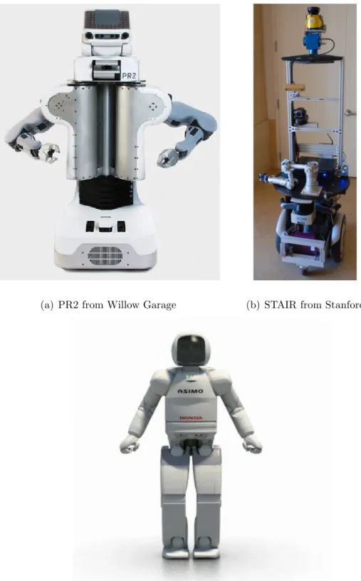
General purpose robots such as Willow Garage’s PR21 and Stanford’s STAIR
robot2 are capable of performing a wide range of tasks such as folding laundry [45],
and unloading the dishwasher [31] (figure 1.1). While many of these tasks will come pre-programmed from the factory, we would also like the robots to acquire new tasks from their human owners. For the general population, this demands a simple and robust method of communicating new tasks. Through this dissertation I hope to promote the use of the partially observable Markov decision processes (POMDP) as a framework for controlling the robot during these task communication phases. The idea is that we represent the unknown task as a set of hidden random variables. Then, if the robot is given appropriate models of the human, it can choose actions that elicit informative responses from the human, allowing it to infer the value of these hidden random variables. I formalize this idea in chapter 2. This approach makes the robot
1http://www.willowgarage.com/pages/pr2/overview 2http://stair.stanford.edu/
an active participant in task communication.3
Note that I distinguish “task communication” from “task execution”. Once a task has been communicated it might then be associated with a trigger for later task execution. This dissertation deals with communicating the details of a task, not commanding the robot to execute a task; i.e. task communication not task execution.
1.1
Dissertation Contents and Contributions
In the following section we review work related to human-robot task-communication and to communication using POMDPs. Chapter 2 presents the framework, with a re-view of partially observable Markov decision processes (POMDPs), including Bayesian Inference, Belman’s equation, and an overview of POMDP solvers. Chapter 3 works through an example of encoding task communication as a POMDP for a simple task. Chapter 4 describes results from a user experiment, which evaluates the proposed POMDP framework. Chapter 5 summarizes the dissertation and outlines future re-search directions. Finally, the appendices present the full state and transition model used in the experiment.
This dissertation makes the following contributions:
• It frames human-robot task communication as a POMDP, a widely used frame-work. This enables the leveraging of techniques developed for the many prob-lems framed as a POMDP.
• It provides an example of framing a task communication problem as a POMDP.
3Though related, this is different from an active learning problem [34], since the interaction in
• It validates the framework through results from a user experiment. The results suggest that the proposed POMDP framework produces robots that are robust to teacher error, that can accurately infer task details, and that are perceived to be intelligent.
1.2
Related Work
1.2.1
Demonstration
Many researchers have addressed the problem of task communication. A common approach is to control the robot during the teaching process, and demonstrate the desired task [10, 30, 23]. The problem for the robot is then to infer the task from examples. My proposed framework addresses the general case in which the robot must actively participated in the communication, choosing actions to facilitate task inference. That said, demonstration is a common and efficient method of communica-tion. Many of these approaches are compatible with the general framework proposed in this dissertation, and would be appropriate when the robot chooses to observe a demonstration (see section 1.3).
1.2.2
Action Selection During Communication
In other work, as in mine, the task communication is more hands off, requiring the robot to choose actions during the communication, with much of the work using binary approval feedback as in my experiment below [44, 2, 13]. The approach pro-posed in this thesis differs in that it proposes the use of a POMDP representation,
while prior work has created custom representations, and inference and action se-lection procedures. This work does introduce interesting task domains, and the task representations may be useful as representations of hypotheses as more complex tasks are considered (see section 5.2.2).
The Sophie’s Kitchen work used the widely accepted MDP representation [40]. An important difference from the approach presented in this dissertation is in the way that actions are selected during task communication. In their work the robot repeatedly executes the task, with some noise, as best it currently knows it. In my proposed approach the robot chooses actions to become more certain about the task. Intuitively, if the goal of the interaction is to communicate a task as quickly as possible, then repeatedly executing the full task as you currently believe it, is likely not the best policy. Instead, the robot should be acting to reduce uncertainty specifically about the details of the task that it is unclear on. In order to generate these uncertainty reducing actions I feel that a representation allowing for hidden state is needed, and I have proposed the POMDP. Unlike an MDP, with a POMDP there can be a distribution over details of the task, and actions can be generated to reduce the uncertainty in this distribution. The purpose of their work was to report on how humans act during the teaching process. As such, it, and much of the work from Social Robotics (section 1.2.4), is relevant for the human models needed in the proposed POMDP.
1.2.3
Control
Substantial work has also been done on human assisted learning of low level control policies, such as the mountain car experiments, where the car must learn a throttle policy for getting out of a ravine [16]. While the mode of input is the same as is used in the demonstration of chapter 3 (a simple rewarding input signal), we are address-ing different problems and different solutions are appropriate. They are addressaddress-ing the problem of transferring a control policy from a human to the robot, where ex-plicit conversation actions to reduce uncertainty would be inefficient, and treating the human input as part of an environmental reward is appropriate. In contrast I am addressing the problem of communicating higher level tasks, such as setting the table, in which case, explicitly modeling the human and taking communication actions to reduce uncertainty is beneficial, and treating the human input as observations car-rying information about the task details is appropriate. The tasks that would be communicated with the proposed POMDP approach do assume solutions to these control problems; such as avoiding obstacles and manipulating objects. In a deployed setting, a robot will need to acquire these control skills in the field. Since a human is present, hopefully these techniques can be employed to help the robot acquire these control skills.
1.2.4
Social Robotics
The area of social robotics, which includes the Sophie’s Kitchen work discussed above, is relevant and provides many insights for the problem of human-robot task communication. Social robotics deals with the class of robots “that people apply a
social model to in order to interact with and to understand”, Cynthia Breazeal [4]. The focus of social robotics research is on identifying important social interactions and demonstrating that a robot can participate in those interactions.
Three examples of these interactions are vocal turn taking, shared attention, and maintaining hidden beliefs about the partner. By encoding rules of vocal turn taking, involving vocal pauses, eye movement, and head movement, Breazeal demonstrated that a robot can converse with a human, in a babble language, smoothly and with few “hiccups” in the flow [3]. Breazeal et al., and Scassellati motivated and demonstrated shared attention, in which the robot looks at the human’s eyes to determine the object of their focus and then looks at that object [5, 33]. Gray et al. demonstrated that a robot can maintain beliefs about the goals and the world state as seen from the conversation partner (these are not beliefs in the probabilistic sense, see section 2.1, the robot tracks the deterministic observable state of the world and the changes that the partner was present to observe; the goals are a shrinking list of the possible states that the partner is attempting to reach.) [9, 6].
The work in social robotics provides a guide for desirable interactions and human models. The hope is to develop robot controllers for which the robot’s actions in these interactions are not scripted rules, triggered by observable state, but are chosen to minimize a global cost function and operate in uncertain environments. The dis-advantages of a set of action rules (situation → action) are that the set is unwieldy to specify and maintain, it can have conflicting rules, and the long term effects of the rules can be hard to predict (no global objective). For an introduction to social robotics, see [4].
1.2.5
Spoken Dialog Managers
A spoken dialog manager is an important component within a spoken dialog system, such as an automated telephone weather information service. The dialog manager receives “speech act” inputs from the natural language understanding com-ponent, tracks the state of the conversation, and outputs speech acts to the spoken language generator component. Like task communication in robotics, a spoken dialog manager often seeks to fill in details of interest from noisy observations, and it can direct the conversation through actions. The current state of the art systems use POMDPs as the representation. As such, the techniques which allow these systems to scale are relevant to human-robot task communication. The two main compo-nents that resist scaling in a POMDP implementation are belief tracking and action planning.
Spoken dialog manager researchers have scaled belief tracking through two tech-niques: factoring and partitioning. In factoring, the details of interest are divided into sets that can be tracked independently [50, 42]. If |A1| is the number of answers to question one and |A2| is the number of answers to question two, then without factor-ing we have|A1||A2| hypotheses to track, with factoring this is reduced to|A1|+|A2|
hypotheses. Unfortunately, there is often a dependency between details of interest which precludes factoring. Partitioning, on the other hand, can handle these depen-dencies. It lumps hypotheses into partitions, each partition contains one or more hypotheses, and tracks the probability of the partitions [46, 51]. For example, if we are interested in the city to report weather for, based on the input so far, the agent might be tracking four hypotheses (Boston, Austin, Houston, and !(Boston, Austin,
or Houston)). Partitioning is effective because we can wait to enumerate hypothesis until there is evidence to support them. It also scales with the availability of process-ing and memory; with more processprocess-ing and memory we can more finely partition the hypothesis space, allowing for more accurate tracking.
The planning problem has been addressed by reducing the problem space over which planning occurs. This is done by mapping the problem into a smaller feature space, perform planning in this space, and mapping the solution back to the original problem space [48, 49]. Using the telephone weather agent as an example of this mapping, the only reasonable confirmation action is to ask confirmation for the most likely city. Thus, the probability of all cities could be mapped to the two element feature vector which contains the probability of the most likely city and, perhaps, the entropy of the remaining cities, vastly simplifying the problem. These techniques have led to spoken dialog systems that can handle very large problem spaces [15, 52]. While these and other techniques are relevant, there are two important distinc-tions between spoken dialog management and human-robot task communication. The first is that the observations in a spoken dialog system are usually in one-to-one cor-respondence with details of interest, which allows for simplified inference through techniques like factoring. In human-robot task communication it is often unclear which task details the observation is relevant to (e.g. a pointing gesture could mean the task involves moving the object you are holding to that location, or it could mean that the task involves picking up another object at that location). The second distinction relates to the the termination of the communication. Most spoken dia-log systems seek to submit the details of interest quickly to another system, which
makes the cost function reasonably easy to specify (penalize an incorrect submission, reward a correct submission, and lightly penalize all non submit actions). Although outside the work presented in this dissertation, in human-robot task communication, the robot’s operation is broader than a single task communication exchange. A task communication exchange is situated within the continuous operation of the robot, and the robot’s actions should factor in the human’s desire to communicate yet an-other task or to start the robot executing a task. Thus, the choice of a cost functions is less obvious. See section 5.2.5 for a discussion of good cost functions for human robot interaction. For an excellent overview of spoken dialog management, see [47].
1.3
Why Control the Communication?
In the task communication framework proposed below the robot plans its actions; i.e. the robot is in control of its actions and chooses those actions in accordance with an objective function. Since this planning adds a significant computational cost, why is it important? The alternative would be for the human to provide demonstrations of the task, either with their own body or by controlling the robot’s body. The robot would still be required to infer the task from the demonstrations, but this would eliminate the additional need for planning.
The benefit of planning is that it makes task communication faster and more accurate:
• faster — With planning, the robot can direct the communication away from details that are obvious to it (perhaps from related tasks), eliminating the time
needed to demonstrate those details. Without planning, the human would need to fully demonstrate all of the details for every task that they teach the robot. • more accurate — With planning, the robot can direct the communication towards details of the task that are not yet clear. Without planning, the teacher can easily omit demonstrations that might clarify a task detail. For example, if the human is teaching the “pour a glass of milk” task, they could easily provide all demonstrations with the glass roughly one foot from the sink, leaving the robot uncertain about the importance of this distance. With planning, the robot could plan to clarify the importance of the distance to from sink.
Both of these benefits have at their core the fact that only the robot knows what the robot knows, and planning can leverage this knowledge.
Note that planning does not preclude demonstrations, but the act of observing the demonstration should be an action that, through planning, is expected to improve communication. If the observed action loses its benefit over time, the robot can interrupt the observation and take a more productive action.
As an example of the benefit of planning in a familiar human setting, we can look at a professor’s office hours. A student may choose to listen to their professor’s expla-nation, but they are still free to interrupt the professor and direct the communication; perhaps informing the professor that they are clear on the aspect that the professor is explaining, but are unclear on another aspect. The ability of the student to direct the communication makes office hours more efficient.
(a) PR2 from Willow Garage (b) STAIR from Stanford
(c) ASIMO from Honda
Figure 1.1: Three examples of modern general purpose robots. PR2 image from http://www.willowgarage.com/pages/pr2/overview, c!Willow Garage. STAIR im-age from http://stair.stanford.edu/ c!Stanford University. ASIMO image from http://world.honda.com/ASIMO/ c!Honda Motor Co.
Framework
2.1
POMDP Review
A partially observable Markov decision process (POMDP) provides a standard way of representing sequential decision problems where the world state transitions stochastically and the agent perceives the world state through stochastic observa-tions. A standard representation allows for the decoupling of problem specification and problem solvers. Once a problem is represented as a POMDP, any number of POMDP solvers can be applied to solve the problem. A POMDP solver takes the POMDP specification and returns a “policy”, which is a mapping from belief states to actions. POMDPs have been successfully applied to problems as varied as au-tonomous helicopter flight [21], mobile robot navigation [29], and action selection in nursing robots [26].
In this section we review the POMDP, including Bayesian inference, Belman’s equation, and the state of the art in POMDP solvers. For additional reading on
POMDPs see [36], [43], and [12].
2.1.1
Definitions
Random variables will be designated with a capital letter or a capitalized word; e.g. X. The values of the random variable will be written in lowercase; e.g. X =x. If the value of a random variable can be directly observed then we will call it an “observable” random variable. If the value of a random variable cannot be directly observed then we will call it a “hidden” random variable, also known as a “latent” random variable. If the random variable is “sequential”, meaning it changes with time, then we will provide a subscript to refer to the time index; e.g. Mt below. A random variable can be multidimensional; e.g. the stateS below is made up of other random variables: M ov, Mt, etc. If a set of random variables contains at least one hidden random variable then we will call it “partially observable”.
P(X) is the probability distribution defined over the domain of the random vari-able X. P(x) is the value of this distribution for the assignment of xto X. P(X|Y) is a “conditional” probability distribution, and defines the probability of a value of
X given a value of Y. A “marginal” probability distribution is a probability dis-tribution that results from summing or integrating out other random variables; e.g.
P(X, Y) :∀x∈X,y∈YP(x, y) =!z∈ZP(x, y, z). When a probability distribution has a
specific name, such as the “transition model” or the “observation model” we will use associated letters for the probability distribution; e.g. T(...) or Ω(...).
2.1.2
POMDP Specification
A POMDP specification is an eight element tuple: $S, A, O, T,Ω, C, γ, b0%. S is the set of possible world states; A is the set of possible actions; O is the set of possible observations that the agent may measure; T is the transition model defining the stochastic evolution of the world (the probability of reaching state s" ∈ S given
that the action a ∈ A was taken in state s ∈ S); Ω is the observation model that gives the probability of measuring an observation o ∈ O given that the world is in a state s ∈ S; C is a cost function which evaluates the penalty of a state s ∈ S
or the penalty of a probability distribution over states (called a belief state b, b : ∀s∈S
"
0≤b(s)≤1 and !s∈Sb(s) = 1#); γ is the discount rate for the cost function; and, finally, b0 is the initial belief state for the robot, i.e. the initial probability distribution over world states. Given a POMDP representation, a POMDP solver seeks a policy π, π(b) :b→a, that minimizes the expected sum of discounted cost.1,
The cost is given byC, the discounting is given byγ, and the expectation is computed using T and Ω.
The state of the robot S should capture all quantities relevant to the decision making process. For example, the state for a path planning robot might consist of the two dimensional position of the robot (S = (X, Y)). An assignment to all of the quantities in S is often called a hypothesis. The number of hypotheses is the number of joint assignments to all quantities in S. A belief state b is a probability distribution over hypotheses; i.e. it assigns a probability to every hypothesis. Often
1Often a reward function is used instead of a cost function, but these are interchangeable;
this is explicitly represented as an array of probabilities, where each element is the probability of one assignment to S. One of these arrays represents one belief state.
b0 might be initialized to a uniform distribution; i.e. each element of the array has the same value: $size(array)1 %.
Figure 2.1: The POMDP world view. In one timestep the agent selects an action and receives an observations from the world. The agent incurs costs associated with its updated belief based the action and the observation. The agent models the world by
T and Ω; the new state is sampled from T, and the observation received is sampled from Ω.
Figure 2.1 depicts the problem that a POMDP represents. An agent performs an action a ∈ A, given this action the world state changes according to the transition model T. Given the new world state, an observation o ∈ O is generated according to the observation model Ω. The agent receives this observation, updates its internal belief about the true world state, and incurs a cost C(b) associated with this new belief. The goal of the agent is to choose actions that minimize the sum of costs over its lifetime, discounted by γ.
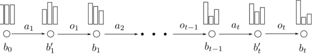
Figure 2.2: An illustration of history as seen from the POMDP perspective. Circles represent beliefs based on a history of actions and observations. The label of the belief is shown below a circle, a cartoon belief histogram is shown above the circle, and arrows are marked by the action or observation that effected the new belief. In one time step the robot receives an action at and an observation ot; the action at
moves the robot’s belief state from bt−1 to the intermediate belief state b"t, and the
observation ot moves the robot’s belief state from the intermediate belief state b" t to
the new belief state bt.
from one timestep to the next and I formally define the equation that the agent seeks to minimize. Note that due to the complexity of literally implementing this update and minimization, nearly all POMDP solvers approximate the update and/or the minimization.
2.1.3
Bayes Filtering (Inference)
The agent starts each timestep with a belief (b0 for timestep zero), it then takes an action and receives a measurement related to the world state at the next timestep. These two pieces of information at+1 and ot+1 are all the agent has to update its belief about the world from bt to bt+1. If we introduce an intermediate belief state
b"
t+1, which captures the belief after incorporatingat+1, but before receiving ot+1, we
get the graphically depicted scene in figure 2.2.
The beliefs can be updated recursively using the following two formulas, which are the Bayes filter update equations.
b"t+1(st+1) = &
st∈S
T(st+1|at+1, st)bt(st) (2.1)
bt+1(st+1) = ηΩ(ot+1|st+1)b"t+1(st+1) (2.2)
b0(s0) is defined to be the probability of the state at time zero; b0(S0) = P(s0).
This is called the prior distribution for the system’s state and is specified ahead of time.
This update from bt to bt+1, given at+1 and ot+1, is called the Bayes filter. Most
filtering algorithms are Bayes filters, notably the Kalman filter and the particle fil-ter [43].
I will now derive equations 2.1 and 2.2, but first an additional notation is helpful. For a temporal random variable X, we denote xt:1 to be an assignment of values to X for each of the timesteps from 1 tot; i.e. (xt, xt−1, xt−2, . . . , x2, x1).
The recursive expression for the belief bt+1(st+1) in terms of the belief bt(st) is
derived as follows:
bt+1(st+1) = P(st+1|at+1:1, ot+1:1) (2.3) = P(ot+1|st+1)P(st+1|at+1:1, ot:1)
P(ot+1|at+1:1, ot:1) (2.4) = P(ot+1|st+1) ! st∈SP(st+1, st|at+1:1, ot:1) P(ot+1|at+1:1, ot:1) (2.5) = P(ot+1|st+1) !
st∈SP(st+1|at+1, st)P(st|at+1:1, ot:1) P(ot+1|at+1:1, ot:1)
(2.6) = ηP(ot+1|st+1)&
st∈S
P(st+1|at+1, st)P(st|at+1:1, ot:1) (2.7)
= ηP(ot+1|st+1)&
st∈S
P(st+1|at+1, st)P(st|at:1, ot:1) (2.8)
= ηΩ(ot+1|st+1)&
st∈S
Line 2.3 is the definition of the belief statebt+1(st+1); i.e. the probability distribution over states given the full action and observation history. Line 2.4 uses Bayes rule to pull out ot+1 from the history and the fact that an observation ot+1 is independent of the history, given the current state st+1. Line 2.5 introduces st using the law of total probability. Line 2.6 uses the definition of conditional probability and the fact that the next statest+1 is independent of the history, given the action takenat+1 and the previous state st (Markov property). Line 2.7 uses the fact that the denominator is not a function of the variable of interest for the probability distribution (st+1), thus it is constant for all assignments to st+1 and we can recover its value after the update; it is one over the sum of the unnormalized distribution. In line 2.8 theat+1 is dropped. This is typically justified for pure filtering problems by saying that future actions are randomly chosen. In a control problem actions are determined by a policy (at+1 =π(bt)). So the explanation is more complicated,
P(st|at+1:1, ot:1) =
P(at+1|st, at:1, ot:1)P(st|at:1, ot:1)
P(at+1|at:1, ot:1) (2.10) = P(at+1|at:1, ot:1)P(st|at:1, ot:1)
P(at+1|at:1, ot:1) (2.11) = P(st|at:1, ot:1) (2.12)
Line 2.10 is from Bayes Rule and 2.11 is because the action at+1 is independent of the true state, since it is chosen based on the belief state bt which is a function only of the history. Finally, in the derivation of bt+1(st+1), line 2.9 substitutes Ω, T, and
bt in place of their definitions.
For implementation we do this update in two steps, one for the action, which leads to an intermediate belief state b"
after incorporating the action but before incorporating the measurement.
b"t+1(st+1) = P(st+1|at+1, at:1, ot:1) (2.13)
= &
st∈S
P(st+1|at+1, st)P(st|at+1, at:1, ot:1) (2.14)
= &
st∈S
P(st+1|at+1, st)P(st|at:1, ot:1) (2.15)
= &
st∈S
T(st+1|at+1, st)bt(st) (2.16)
To incorporate the observation into the belief we plug equation b"
t+1(st+1) into
equation (2.9). This gives us our two recursive update equations mentioned above:
b"t+1(st+1) = &
st∈S
T(st+1|at+1, st)bt(st) (2.1)
bt+1(st+1) = ηΩ(ot+1|st+1)b"t+1(st+1) (2.2)
2.1.4
Belman’s Equation (Planning)
Intuitively, certain belief states are more attractive to the agent then others. Not just because they receive a low immediate cost C(b) but because they are on a path that will have a low sum of costs.
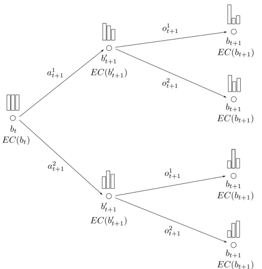
LetEC(b), formally defined below, represent how much the agent dislikes a belief; i.e. the immediate cost plus the long run cost. Given EC(bt+1) for each belief state one time step away, i.e. reachable by one action and one observation, depicted in figure 2.3, we can ask two important questions: 1) what action should the robot take in the current state?, and 2) what is EC(bt) for the current beliefbt?
Referencing figure 2.3, these questions assume that we are given the fourEC(bt+1) for each of the four leaf nodes. We can compute the EC(b"t+1) for the two b"t+1 by
Figure 2.3: A belief tree expanded one time step into the future for a POMDP with two actions (a1, a2) and two observations (o1, o2). The belief label bi is shown below
the node, a cartoon histogram of the belief is shown above the node, and the expected sum of discounted costs EC(bi) from the belief bi onward is shown below the belief.
The EC(bi) are useful for choosing optimal actions. The actions and observations that effect the beliefs are shown on their arrows. Beliefs are propagated from the left to the right according to the Bayes filter equations (2.1 and 2.2). EC(bi) are
propagated from right to left using Belman’s equation (2.22)).
node.
EC(b"t+1) = &
ot+1
p(ot+1|at+1, at:1, ot:1)EC(bt+1) (2.17)
= E
ot+1
EC(bt+1) (2.18)
The optimal action is then just the action that leads to the b"
t+1 with the smallest EC(b" t+1). at+1 = arg min at+1 EC(b"t+1) (2.19) = arg min at+1 E ot+1 EC(bt+1) (2.20)
AndEC(bt) is the immediate costC(bt) plus the EC(b"
t+1) under the optimal action,
discounted: EC(bt) = C(bt) +γmin at+1 EC(b"t+1) (2.21) = C(bt) +γmin at+1otE+1 EC(bt+1) (2.22)
Equation 2.22 is called Belman’s equation and is the recursive constraint that guar-antees optimal action selection.
An intuitive, though computationally demanding, POMDP solver would, starting at the current belief, roll out the action selection tree of figure 2.3 to a finite horizon
T. For each leafbT it could approximate EC(bT) as
EC(bT) =C(bT). (2.23)
It could then back up theEC using Belman’s equation (equation 2.22; taking expec-tations of observation branches and minimums of action branches), untilEC(bt+1) for all beliefs bt+1 had been computed. Finally it would select the optimal action using equation 2.20.
Derivation
I now derive why Belman’s equation enforces optimal action selection, and I for-mally define EC in the process. By definition, the optimal next action is the action that minimizes the expected sum of discounted costs over action and observation futures:
at+1 = arg min
at+1 E ot+1 ' C(bt+1) +γmin at+2 oEt+2 ' C(bt+2) +γmin at+3 oEt+3 [. . .] (( (2.24) We define EC(bt+1) as the quantity in the outer square brackets,
EC(bt+1) = C(bt+1) +γmin at+2otE+2 ' C(bt+2) +γmin at+3otE+3 [. . .] ( . (2.25)
We can express EC(bt+1) recursively in terms of EC(bt+2) by substituting EC(bt+2) into equation 2.25 to get,
EC(bt+1) = C(bt+1) +γmin
at+2otE+2
EC(bt+2). (2.22)
This is Bellman’s equation. Substituting EC(bt+1) into the optimal action equation 2.24, gives,
at+1 = arg min
at+1 E ot+1
EC(bt+1). (2.20)
Thus, if we haveEC(bi) for which Belman’s equation holds, then the actions selected by equation 2.20 are optimal.
Lastly, in Belman’s equation we take an expectation over observations (Eot+1EC(bt+1)),
E ot+1
EC(bt+1) = &
ot+1∈O
p(ot+1|at+1, ot:1, at:1)EC(bt+1) (2.26)
where
p(ot+1|at+1, ot:1, at:1) = &
s!∈S
P(ot+1|s")P(s"|at+1, ot:1, at:1) (2.27)
= &
s!∈S
P(ot+1|s")&
st∈S
P(s"|at+1, st)P(st|ot:1, at:1) (2.28)
= & s!∈S Ω(ot+1|s")& st∈S T(s"|at+1, st)b(st) (2.29)
2.1.5
POMDP Solvers
The goal of a POMDP solver is to choose an action a for a belief state b that minimizes the expected sum of discounted rewards (equation 2.24). POMDP solvers can be classified into two broad categories, offline or online. An offline solver does all of its processing before the agent is run and produces a policy π(b), which maps every belief state b to an action a. An online solver uses the time between actions to compute the next action at+1 given the current belief state bt.
Both offline and online solvers have their tradeoffs. An offline solver generally has more time for computation but the computation must be spent on a range of belief states, since the policy must specify an action for any belief state. Also, since the policy returned by an offline solver is typically a simple mapping, it can be rapidly evaluated by the running agent, which can be important if the processing time between actions is limited. In contrast, an online solver has less time for computation (only the time between actions) but it can focus this processing on the immediately relevant
belief states.
There is strong overlap between offline and online approaches. Advances in one can often be applied to others. And, in general, offline processing policies can be used to improve the quality of online policies. The best performing systems make use of all of the online processing available and augment this with a policy from an offline solver, see the heuristic solver below. Here is a brief overview of several offline and online POMDP solvers.
Offline Solvers
Most offline solvers (included all but one of the reviewed solvers) solve the POMDP by seeking the expected cost for all belief statesEC(b) (equation 2.25). The optimal action can then be determined by either direct lookup (often the optimal action that lead to minimizingEC(b) is stored), or by using equation 2.20 to compute the optimal action in terms of EC(b).
• exact expected cost — Early on it was shown that the expected cost of a belief state bt can be expressed as a concave linear function of bt, where the parameters are derived from the expected cost for one time step in the future
ECt+1 (which is also a convex linear function of the belief state bt+1 [35]). By starting with EC(b) = C(b), and repeatedly computing the expected cost one timestep early, as the number of updates goes to infinity, the expected cost approaches the true expected cost (equation 2.25). Unfortunately the number of linear equations that make up the expected cost grows exponentially with each update, thus this approach is only appropriate in extremely simple domains.
• point based — Point based POMDP solvers also solve Belman’s equation (equation 2.22), but only for a small set of beliefs [18]. Implementations vary on how they select the belief set. The distribution of the belief set is critical to the accuracy of the solution. In general, the more beliefs in the set, the more accurate the estimate of expected cost, but, also, the more processing required. Two recent algorithms using the point based approach are PBVI [25] and Perseaus [37].
• upper bound — Some solvers return strict upper or lower bounds for the expected cost function EC(b). These can be useful as heuristics for online solvers. One example of an upper bound solver evaluates the expected cost of always executing the same action, called a “blind” policy [11]. Since these policies are independent of observations, their expected cost can be solved with an MDP-like value iteration. EC(b) is then computed in the same way as the MDP lower bound example below. Even a bound as loose as this can be helpful as a heuristic [28]. A tighter upper bound can be achieved using a point based solver, but this comes at the cost of more computation.
• lower bound— A lower bound solver computes a strict lower bound onEC(b). One example of a lower bound solver is to solve the underlying MDP, which make the assumption that the state is observable [17]. Let ECM DP(s) be the
expected cost under this assumption for the state s. We then compute EC(b) asEC(b) = !sECM DP(s)b(s). Solving the underlying MDP results in a lower
bound because it ignores uncertainty, and is thus overly optimistic. Recent lower bound POMDP solvers include QMDP [17], and FIB [11].
• policy search — A policy search method directly modifies a parameterized policy. If we can efficiently compute the expected cost of a policy, and if the pa-rameterized policy is differentiable, then we can apply gradient descent methods directly on the policy [1]. Applications where a differentiable policy is appropri-ate are more common in control than in artificial intelligence. If the conditions are met, a policy search algorithm can be an efficient solver.
• permutable POMDPs— A permutable POMDP is a sub-class of POMDPs [7]. In many applications the optimal policy only depends on the shape of the cur-rent belief and not on the value of a state variable. For example, for a telephone directory agent, the agent may be seeking the first name of the person you want to reach. The optimal policy is independent of the value of the first name. If the belief were in a particular shape, the optimal policy would “ask confirmation of the most probable value for the first name”; whether to ask this question would not depend on the value of the most probable first name. Solvers can take advantage of the permutable property by computing expected costs only for a sorted belief state. Because the states are permutable, this also provides the expected cost for any permutation of that belief state. Simple transforma-tions to and from the sorted belief state are used online to extract the expected cost for the current belief state. Doshi and Roy showed that this results in an exponential reduction in the belief space, making the POMDP easier to solve [7]. In their implementation, they wrapped these transformations within a point based value iteration solver, but it should be broadly applicable to most POMDP solvers when the POMDP has the requisite permutable structure.
Online Solvers
Most online solvers, including those presented here, recommend an action by ex-panding the belief tree (figure 2.3), evaluating the expected cost of leaf nodes, and backing them up, using Belman’s equation (equation 2.22), to the current node. The action recommended is the very next action that resulted in the current belief node’s minimum value. These approaches differ in how they expand this tree, as described below.
• branch and bound — Branch and bound techniques maintain a lower bound and an upper bound on EC for each each node in the tree [24]. If the lower bound for one action nodea" is higher than the upper bound for another action, then we can stop exploring all branches below a", since the other action is guaranteed to result in a lower EC. The full process is as follows: the tree is expanded to a depth; the upper and lower bounds are computed for the leaf nodes (typically using an offline solution); these bounds are propagated up the tree; branches are then pruned beyond actions that will never be taken; and the the process repeats, expanding the tree from the remaining leaf nodes. This pruning saves significant computation, but we can do even better; see the heuristic solver below.
• monte carlo— A monte carlo solver also expands the belief tree, but stochas-tically traverses observation branches based on the probability of that observa-tion [19]. This is effective because it steers the search towards observaobserva-tions that are more likely.
• heuristic — Heuristic solvers are similar to branch and bound solvers in that they maintain an upper and lower bound for each node’s expected cost, but unlike branch and bound they do not uniformly expand leaf nodes. Heuristic solvers apply a heuristic function to all leaf nodes and expand the node with the best value. One effective heuristic is the contribution of that leaf nodes error (upper bound - lower bound) to the root node’s error [27]. A leaf node’s error contributes to the root’s error in proportion to the discounted probability of reaching that leaf. This heuristic encourages the expansion of leaf nodes that will aid in the immediate decision of which action to take.
A good overview with references to further reading on POMDP solvers can be found in Ross et al. [28]. The current state of the art in POMDP solvers are heuristic methods with simple upper and lower bounds computed by an offline solver. For human-robot task communication in complex task domains, a reasonable option for a POMDP solver would be the combination of a heuristic solver (using “blind” and QMDP for bounds) with the approach of mapping to a reduced planning space (from the spoken dialog manager work in section 1.2). If the number of observations makes the evaluation of all leaf nodes intractable, then the monte carlo approach could be used to select a subset of leaf nodes to evaluate for expansion.
2.2
Task Communication as a POMDP
This dissertation proposes the use of a POMDP for representing the problem of a human communicating a task to a robot. Specifically, for the elements of the POMDP tuple $S, A, O, T,Ω, C, γ, b0%, the partially observable state S captures the
details of the task along with the mental state of the human (helpful for interpreting ambiguous signals); the set of actions A capture all possible actions of the robot during communication (for example words, gestures, body positions, etc.); the set of observations O capture all signals from the human (be they words, gestures, buttons, etc.); and the cost function C should encode the desire to minimize uncertainty over the task details inS. The transition model T, the observation model Ω, the discount rate γ, and the initial belief state b0 fill their usual POMDP roles.
The next chapter provides a demonstration of representing a human-robot task communication problem as a POMDP, including examples of T, Ω, and b0.
2.2.1
Choice of Cost Function
I say above that the cost function C should encode the desire to minimize uncer-tainty over the task details inS; i.e. the cost function should penalize uncertainty. As mentioned in section 1.2.5, in the field of spoken dialog managers, the cost function is chosen to penalize communication time and incorrect submission of the quanti-ties being communicated, and reward correct submissions. The system still explores (reducing uncertainty about the quantities), but only in pursuit of timely, correct submissions. Unlike an uncertainty penalizing cost function, this cost function has the added benefit of being linear in the belief state, which is a requirement of some POMDP solvers. Eventually, the robot will be in a situation where communication must be terminated in order to perform another function, such as task execution; but for this dissertation, the setting is solely task communication. As such, a terminal submit action is not appropriate, since it would end the robot’s actions and prevent
further communication. An uncertainty penalizing cost function is promoted because it focuses the robot’s actions on task communication, which is the problem at hand, with the added benefit of being parameter free. That said, I do view this as a tem-porary cost function until a more encompassing cost function is developed for the broader problem of task communication and task execution (see section 5.2.5).
Demonstration
In this chapter I provide a demonstration of representing a human-robot task communication problem as a POMDP. The representation is what is used in the experiment in chapter 4. The task to be communicated relates to a simulated envi-ronment shown in figure 3.1. As such we begin with a description of the simulator and its virtual world.
3.1
Simulator
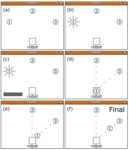
The virtual world is shown in figure 3.1. It consists of 3 balls and the robot, displayed as circles and a square (3.1.a). The robot can “gesture” at balls by lighting them (3.1.b), it can pick up a ball (3.1.d), it can slide one ball to one of four distances from another ball (3.1.e), and it can signal that it knows the task by displaying “Final” (3.1.f). The experiment in chapter 4 will contain trials in which a human acts as the robot. For these comparison trials the robot actions are controlled by left
Figure 3.1: Typical human-robot interactions on the simulator. (a) The state all trials start in; the square robot, holding no balls, surrounded by the three balls. (b) The robot lighting one of the balls, as if to ask, “move this?” (c) The human teacher pressing the keyboard spacebar, displayed in the simulator as a rectangle, and used to indicate approval with something the robot has done. (d) The robot holding one of the balls, the four relative distances are displayed to the remaining two balls. (e) The robot has slid one of the balls to the furthest distance from another ball. (f) the robot has displayed “Final”, indicating that it knows the task, and that the world is currently in a state consistent with that task.
and right mouse clicks on the objects involved in the action; e.g. right click on a ball to light it or turn off the light, left click on a ball to pick it up, etc. In this simulator
the teacher input is highly constrained; the teacher has only one control and that is the keyboard spacebar, visually indicated by a one half second rectangle (3.1.c), and is used to indicate approval with something that the robot is doing or has done. The simulator is networked so that two views can be opened at once; this is important for the comparison trials, where the human controlling the robot must be hidden from view.
Timesteps are 0.5 second long, i.e. the robot receives an observation and must generate an action every 0.5 seconds. The simulator is free running, so, in the com-parison trials where the human controls the robot, if the human does not select an action, then the “no action” action is taken. “no action” actions are still taken in the case of the POMDP-controlled robot, but they are always intentional actions that have been selected by the robot. I provide enough processing power so that the POMDP-controlled robot always has an action ready in the allotted 0.5 seconds. The simulated world is discrete, observable, and deterministic.
3.2
Toy Problem
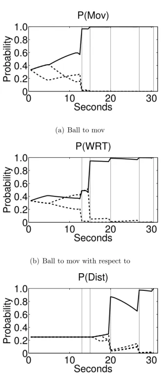
The problem we wish to encode is as follows. A human teacher will try to com-municate, through only spacebar presses, that a specific ball should be at a specific distance from another specific ball. Spacebar presses from teacher should be inter-preted by the robot as approval of something that it is doing. The robot has to infer the relationship the teacher is trying to communicate from the spacebar presses. When the robot thinks it knows the relationship, it should move the world to that relationship and display “Final” to the teacher.
Figure 3.1 shows snap shots from a possible communication trial. The robot “questions” which ball to move (3.1.b), the teacher indicates approval (3.1.c), the robot picks up the ball (3.1.d), the robot “questions” which ball to move the one it is holding to (not shown), the robot slides the ball toward another ball (3.1.e), the teacher approves a distance or progress toward a distance (not shown), and, after further exploration, the robot indicates that it knew the task by displaying “Final” (3.1.f).
Although this problem is simplistic, a robot whose behaviors consist of chainings of these simple two object relationship tasks could be useful; e.g. for the “set the table” task: move the plate to zero inches from the placemat, move the fork to one inch from the plate, move the spoon to one inch from the fork, etc.
I chose the spacebar press as the input signal for the demonstration and for the experiment because it carries very little information, requiring the robot to infer meaning from context, which is a strength of this approach. For a production robot, this constrained interface should likely be relaxed to include signals such as speech, gestures, or body language. These other signals are also ambiguous, but the simplicity of a spacebar press made the uncertainty obvious for the demonstration.
3.3
Formulation
In this section I formulate this problem as a POMDP. This is only one of many possible formulations. It is perhaps useful to note that the formulation presented here, and used in the user experiment below, was the first attempt; neither the structure nor the parameters needed to be adjusted from my initial guesses. This suggests that
the proposed approach is reasonably insensitive to modeling decisions.
3.3.1
State (
S
)
The state S is composed of hidden and observable random variables. The task that the human wishes to communicate is captured in three hidden random variables
M ov, W RT, and Dist. M ov is the index of the ball to move (1−3). W RT is the index of the ball to move ball M ov with respect to. Dist is the distance that ball
M ov should be from ball W RT.
The state also includes a sequential hidden random variable, Mt, for interpreting the observations Ot. Mt takes on one of five values: (waiting, mistake, that mov,
that wrt, orthat dist). A value ofwaitingimplies that the human is waiting for some reason to press the spacebar. A value of mistake implies that the human acciden-tally pressed the spacebar. A value of that mov implies that the human pressed the spacebar to indicate approval of the ball to move. A value of that wrt implies that the human pressed the spacebar to indicate approval of the ball to move ball M ov
with respect to. A value of that dist implies that the human pressed the spacebar to indicate approval of the distance that ball M ov should be from ball W RT. In addition to these hidden random variables, the state also includes observable random variables for the physical state of the world; e.g. which ball is lit, which ball is being held, etc.
Finally, the state includes “memory” random variables for capturing historical information, e.g. the last time step that each of the balls were lit, or the last time step that M =that mov. The historical information is important for the transition
model T. For example, humans typically wait one to five seconds before pressing the spacebar a second time. In order to model this accurately we need the time step of the last spacebar press. See appendix B for a detailed description of the full state along with examples of the observable state variables for several configurations of the world.
state Mov WRT Dist M
$world state variables% $historical variables%
3.3.2
Actions (
A
)
There are six parameterized actions that the robot may perform. Certain actions may be invalid depending on the state of the world. The actions are: noa, for performing no action and leaving the world in the current state; light on(index) or light of f(index), for turning the light on or off for the ball indicated by index;
pick up(index), for picking up the ball indicated by index;release(index), for putting down the ball indicated by index; and slide(index 1, distance, index 2), for sliding the ball indicated by index 1 to the distance indicated by distance relative to the ball indicated by index 2. Note that only a few actions are valid in any world state; for example,slide(index 1, distance, index 2) is only valid if ballindex 1 is currently held or currently at a distance from ballindex 2 and ifdistanceis only one step away from the current distance. See appendix C.1 for effects of these actions.
actions noa
light on(index) light of(index) pick up(index) release(index)
slide(index 1, distance, index 2)
3.3.3
Observations (
O
)
An observation takes place at each time step and there are two valid observations:
spacebar or no spacebar, corresponding to whether the human pressed the spacebar on that time step.
observations spacebar no spacebar
3.3.4
Transition Model (
T
)
A transition model gives the probability of reaching a new state, given an old state and an action. In this example, M ov, W RT, and Dist are non-sequential random variables, meaning they do not change with time, so T(M ov = i, ...|M ov = i, ...) = 1.0. The transition model for the physical state of the virtual world is also trivial, since the virtual world is deterministic.
The variable of interest in this example for the transition model is the sequential random variable M that captures the mental state of the human (waiting, mistake,
that mov, that wrt, orthat dist). The transition model was specified from intuition, but in practice I envision that it would either be specified by psychological experts, or
Figure 3.2: This is an illustration of part of the transition modelT. Here I show the probability that the human will signal their approval (via a spacebar press) of the ball to be moved, T(M =that mov|M ov =i, ...), where, in this hypothesis, the ball to be moved is ball i. (a) once the robot has lit balli, the probability increases from zero to a peak of 0.1 over 2 seconds. (b) after the light has turned off there is still probability of an approving spacebar press, but decreasing over 2 seconds. (c) If the teacher has signaled their approval (M =that mov), then the probability resets. The structure and shape of these models was set from intuition.
learned from human-human or human-robot observations [41, 39]. For the experiment I set the probability thatM transitions tomistake from any state to a fixed value of 0.005, meaning that at any time there is a 0.5% chance that the human willmistakenly
press the spacebar indicating approval. I define the probability that M transitions to that mov, that wrt, or that dist as a table-top function, as shown in figure: 3.2. I set the probability that M transitions to waiting to the remaining probability;
T(M = waiting) = 1−T(M = mistake ∨that mov∨ that wrt∨that dist). See appendix C for the full transition model.
3.3.5
Observation Model (
Ω
)
The observation model I have chosen for this problem is a many to one determin-istic mapping: P(O =spacebar|M) = 0.0 if M =waiting 1.0 otherwise
Note that this deterministic model does not imply that the state is observable since, given O = spacebar, we do not know why the human pressed the spacebar,
M = (? mistake∨that mov∨that wrt∨that dist). 1
3.3.6
Cost Function (
C
)
As mentioned earlier, the cost function should be chosen to motivate the robot to quickly and accurately infer what the human is trying to communicate. In our case this is a task captured in the random variables M ov, W RT, andDist. The cost function I have chosen is the entropy of the marginal distribution over M ov, W RT, and DIST:
C(p) =−&
x
p(x)·log(p(x)). (3.1)
Where p is the marginal probability distribution over M ov, W RT, and Dist, and x
takes on all permutations of the value assignments to M ov, W RT, and Dist.
Since entropy is a measure of the uncertainty in a probability distribution, this cost function will motivate the robot to reduce its uncertainty overM ov,W RT, and
Dist, which is what we want.
3.3.7
Discount Rate (
γ
)
γ is set to 1.0 in the experiment, meaning that uncertainty later is just as bad as uncertainty now. The valid range ofγ for a POMDP solver evaluating actions to an infinite horizon is 0≤γ <1.0, but the solver only evaluates to a 2.5 second horizon. In practice, the larger the value of γ, the more willing the robot is to defer smaller gains now for larger gains later.
3.3.8
Initial Belief (
b
0)
The initial distribution b0 over the joint values of the hidden random variables
M ov, W RT, Dist, and M are set as follows. M0 is assumed to be equal towaiting. All 24 (3×2×4×1) hypotheses, constructed from the permutations of the hidden random variables (M ov = (1,2,3), W RT = (1,2,3), Dist = (20,40,60,80), M =
waiting), are set to the uniform probability of 1/24.
3.3.9
Action Selection
The problem of action selection is the problem of solving the POMDP. As de-scribed in section 2.1.5, there are many established techniques for solving POMDPs [20, 28]. Given the simplicity of the world and the problem, I can take a direct approach. The robot expands the action-observation tree (figure 2.3) out 2.5 seconds into the future, and takes the action that minimizes the sum of expected entropy over this tree. This solution is approximate, since the system only looks ahead 2.5 seconds, but, as I will show in chapter 4, it results in reasonable action selections for the toy problem used in the demonstration and experiment.
When the marginal probability of one of the assignments to M ov, W RT, and
Dist is greater than 0.98 (over 98% confident in that assignment), the robot moves the world to that assignment and displays “Final”.2
2This termination is outside of the proposed POMDP approach of the dissertation. It was
implemented in order to collect data in the experiment. The dissertation deals only with task communication, not with termination of communication to perform some other function. In a strict implementation of the proposed approach, the robot would never stop acting to reduce its uncertainty about the task. See section 5.2.5 for future work on the integration of task communication and task execution modes
Performance
4.1
Experiment
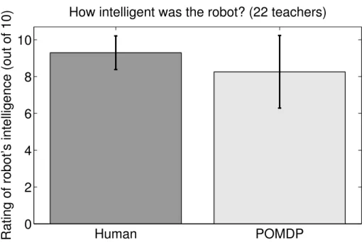
The experiment consisted of multiple trials run on the simulator described in section 3.1, where each trial was one instance of the problem described in section 3.2. In half of the trials the virtual robot was controlled by the POMDP described in section 3.3, and in the other half the virtual robot was controlled by a human hidden from view. At the beginning of each trial the teacher was shown a card designating the ball relationship to teach. The robot, either POMDP or human controlled, had to infer the relationship from spacebar presses. When the robot was confident about the desired relationship it would move the world to that relationship and end the trial by displaying “Final” to the teacher. The teacher would then indicate on paper whether the robot was correct and how intelligent they felt the robot in that trial was.
The experiment involved 26 participants, consisting of undergraduate and grad-uate students ranging in age from 18 to 31 with a mean age of 22. Four of the