Global 3D Non-Rigid Registration of Deformable
Objects Using a Single RGB-D Camera
Jingyu Yang,
Senior Member, IEEE
, Daoliang Guo, Kun Li,
Member, IEEE
, Zhenchao Wu, Yu-Kun
Lai,
Member, IEEE
Abstract—We present a novel global non-rigid registration method for dynamic 3D objects. Our method allows objects to undergo large non-rigid deformations, and achieves high quality results even with substantial pose change or camera motion between views. In addition, our method does not require a template prior and uses less raw data than tracking based methods since only a sparse set of scans is needed. We compute the deformations of all the scans simultaneously by optimizing a global alignment problem to avoid the well-known loop closure problem, and use an as-rigid-as-possible constraint to eliminate the shrinkage problem of the deformed shapes, especially near open boundaries of scans. To cope with large-scale problems, we design a coarse-to-fine multi-resolution scheme, which also avoids the optimization being trapped into local minima. The proposed method is evaluated on public datasets and real datasets captured by an RGB-D sensor. Experimental results demonstrate that the proposed method obtains better results than several state-of-the-art methods.
Index Terms—3D scanning, global registration, non-rigid de-formation, large dede-formation, depth camera, surface reconstruc-tion.
I. INTRODUCTION
D
YNAMIC 3D reconstruction, which aims to recover dynamic scenes by capturing videos using a single or multiple cameras, becomes increasingly popular in computer graphics and computer vision [1]–[4]. With the availability of commodity depth cameras, e.g., Microsoft Kinect, it is easier and cheaper to reconstruct the shape and texture of a 3D scene using a single RGB-D camera. This has many applications [5], [6], such as 3D printing, gaming, and movie production, to name a few. However, reconstruction results by KinectFusion [7] for deformable objects have serious drifting artifacts, because a static model is generally assumed. Besides, the point clouds captured by depth cameras are usually pol-luted by serious noise and outliers. Hence, it remains a hugeCopyright c 2019 IEEE. Personal use of this material is permitted. However, permission to use this material for any other purposes must be obtained from the IEEE by sending an email to [email protected]. This work was supported in part by the National Natural Science Foundation of China (Grant 61571322 and Grant 61771339), and Tianjin Research Program of Application Foundation and Advanced Technology under Grant 18JCYBJC19200.
Jingyu Yang and Daoliang Guo are with the School of Electrical and Information Engineering, Tianjin University, Tianjin 300072, China.
Kun Li and Zhenchao Wu are with the Tianjin Key Laboratory of Cognitive Computing and Application, College of Intelligence and Computing, Tianjin University, Tianjin 300350, China.
Yu-Kun Lai is with the School of Computer Science and Informatics, Cardiff University, Wales, UK.
Corresponding author: Kun Li ([email protected])
challenge to reconstruct dynamic 3D scenes using a single RGB-D camera.
To achieve dynamic 3D reconstruction, several research groups have set up multi-camera systems [8], [9]. However, practical applications of such systems are limited, due to high cost, complex maintenance, and lack of portability. To reduce system sizes, some methods use fewer cameras with depth cues [10]–[12]. Using a single camera is cheaper but the problem becomes more ill-posed. A template prior is usually used to reduce the difficulty [3], [13], [14]. However, using a prior template restricts the captured target as they can pre-scane.g.a deformable object, but cannot model deformations beyond the prior template, such as facial expressions and loose clothing. Some methods try to achieve dynamic 3D reconstruction using a single camera without a template prior. Non-rigid structure from motion methods [15]–[17] aim at recovering dynamic 3D shapes from multi-frame 2D images, but they cannot deal with large scale cases. Alternative methods [18]–[20] based on tracking and fusion of RGB-D sequences of non-rigidly deforming objects are proposed, but small deformation be-tween two neighboring viewpoints (time instances) is generally assumed. To our knowledge, few work in the literature allows large motions of the subject between different viewpoints using a single camera, which happens commonly for snapshot or high speed motion capture.
In this paper, we propose a method for global non-rigid registration and reconstruction of deformable objects with a single RGB-D camera without a template prior. The motion of the object between different viewpoints can be very large. Naive solutions of applying pairwise non-rigid registration in succession lead to error accumulation and the well-known loop closure problem. To address this, we compute the deformations of all the scans simultaneously by optimizing aglobal align-ment problem. We introduce an as-rigid-as-possible (ARAP) constraint to the sparse non-rigid registration framework to eliminate the shrinkage problem of the deformed models when overlapping regions are small and the problem would otherwise be underconstrained. We also design a coarse-to-fine multi-resolution scheme to improve efficiency and robustness. The proposed method is evaluated on public datasets and real datasets captured by an RGB-D sensor. The results demon-strate that the proposed method obtains better results than the state-of-the-art methods.
The main contributions of this work are summarized as follows:
• We propose a global optimization method for reconstruc-tion of deformable objects with large moreconstruc-tions, which is
robust to noise and outliers, and avoids the loop closure problem.
• We design a coarse-to-fine multi-resolution scheme to
avoid the optimization being trapped into local minima, which also helps to attack large scale problems that would otherwise be prohibitively expensive (in terms of computation and storage costs).
• We introduce an ARAP constraint to the sparse non-rigid registration framework, which eliminates the shrinkage problem of the deformed models.
Preliminary results of this work were reported in a confer-ence paper [21]. In addition to more thorough discussions and literature review, the algorithm details are now provided and experimental validation is substantially extended, including quantitative evaluation, evaluation on more datasets, and com-parison with more methods. We first summarize previous work in Sec. II. Then, in Sec. III, we present our global registration framework, including several constraint terms and the overall optimization function. The solution to the optimization func-tion is presented in Sec. IV. Finally, we provide experimental results in Sec. V and conclude this paper in Sec. VI.
II. RELATEDWORK
In this section, we review recent related work in 3D recon-struction.
A. 3D Reconstruction With Multi-Cameras
Several groups have set up multi-camera systems, in which drifting is not a concern because a relatively complete model is captured at each frame. Starck et al. [8] design a system to reconstruct a full human body using 16 cameras, which requires careful positioning of cameras to obtain better raw data. Aguiar et al. [9] build a sparsely sampled system of eight cameras to capture the shape and motion of 3D objects by effectively combining the power of surface-based and volume-based shape deformation techniques. With multiple high-speed cameras, Vlasic et al. [22] design a system for high-resolution capture of moving 3D objects at high details using a photometric stereo light stage. Gallet al.[23] propose an approach based on a multi-view video sequence, which captures the performance of a human or an animal from an articulated template model and silhouettes, and the non-rigid temporal deformation of the 3D surface is then recovered. Liet al.[24] build a dome system with 20 cameras to synchronously capture and recover the dynamic shape and texture of arbitrary objects using a variational multi-view stereo method and a volumetric deformation method. To reduce the number of required cameras, some methods use depth cameras. Tong et al. [10] scan a 3D full human body model using three Kinect cameras, but the method assumes that the person keeps still. Yeet al.[11] use three hand-held Kinects to reconstruct human skeletal poses, deforming surface geometry and camera poses by deforming template models, which generates relatively fine results. Douet al.[12] scan and track deforming objects using fusion of dynamic input from an eight-Kinect rig, by deform-ing a human template. Collet et al.[25] use over 30 RGB-D cameras and a large studio setting with a green screen and
controlled lighting to produce extremely high quality results. Lin et al. [26] optimize the placement of multiple Kinect sensors to achieve the desired scanning accuracy, leading to an effective configuration with 16 RGB-D cameras. Dou et al.[27] design an approach for live performance capture from eight RGB-D sequences, which is robust to large frame-to-frame motion and topology changes, and generates compelling reconstruction results in real-time.
B. 3D Reconstruction With a Single Camera
Considering the high cost and the difficult maintenance of multi-camera systems, monocular approaches become more and more popular. Some methods focus on scanning persons with a fixed pose. Weiss et al. [28] propose to estimate a parametric model of the human shape combining low-resolution image silhouettes with coarse range data. Cui et al. [29] capture a full 3D human body model using a single depth camera, which presents fine results, but limits the user to keep a ‘T’ pose. Li et al.[30] adopt a more general non-rigid registration framework which allows a wider range of poses, which demonstrates compelling results but still requires users to keep the same pose. Dou et al. [31] develop a 3D scanning system which allows a considerable amount of deformations during scanning and shows fine results. However, large deformation between two neighboring viewpoints (time instances) is not allowed.
To reconstruct a dynamic scene using a single camera, non-rigid structure from motion methods are used to recover dynamic 3D shapes from multi-frame 2D images [15]–[17]. However, these methods normally are not able to recover 3D shapes with a large number of vertices. To handle this, some methods capture a static pre-scan as a template prior [9], [12], [23], [32]. Li et al. [33] reconstruct the geometry and motion of complex deforming shapes by using a smooth template that provides a crude approximation to the scanned object and serves as a geometric and topological prior. Zhang
et al. [14] build a personalized parametric model using a single depth sensor, which can produce dynamic models with a generic human template. Zollh¨ofer et al. [13] use a single self-contained stereo camera unit to generate spatio-temporally coherent 3D models, which also starts by scanning a smooth template model of the object using KinectFusion and registers the template to the sequences. In particular, it is able to produce compelling reconstruction models for palms and faces. Guo et al.[3] reconstruct non-rigid geometry and motions from a single-view depth input captured by a depth sensor, which also uses a template prior and presents fine results. However, scanning a template model in advance is inconvenient and impractical for many applications.
Some methods try to achieve dynamic reconstruction using a single camera without a template prior. Liao et al. [34] reconstruct complete 3D deformable models over time by a single depth camera, which is able to reconstruct visually plausible 3D surface deformation results. However, it assumes that the deformation is continuous and predictable in a short temporal interval. Newcombeet al.[20] design a dense SLAM system, which is able to reconstruct non-rigidly deforming
scenes in real-time. Innmann et al. [19] use sparse RGB feature matching to make the tracking system robust to small geometric variation. Dou et al. [18] propose a 360◦ perfor-mance capture system that can reconstruct arbitrary non-rigid scenes in real-time. However, all the methods have the same limitation that small deformation between the neighboring views (frames) is assumed.
C. Shape Registration for 3D Reconstruction
In 3D reconstruction, registration methods are developed to align scans from multiple views with substantial movement, including rigid and non-rigid registration methods [35]. The former assumes that the object only undergoes rigid body transformation [36]–[38], whereas the latter considers more general deformable models, and is thus more suitable for reconstruction of deformable objects. Typical non-rigid reg-istration methods [39] generalize the iterative closest point (ICP) method from rigid registration, and follow a similar paradigm that alternately optimizes correspondences based on the closest point criterion and local transformations according to the updated correspondences. Recent work introduces var-ious effective data and regularization terms to the non-rigid ICP framework [40]–[44] to improve accuracy and robustness of registration. However, such existing non-rigid registration methods are based on pairwise registration. Applying them to multiple scans in succession leads to error accumulation and the loop closure problem, i.e., when a sequence of scans forms a loop, the last scan fails to align with the first scan due to accumulated drifting.
In this paper, we propose a global non-rigid registration framework based on sparse priors as they are robust to noise and outliers. Multiple scans are aligned simultaneously, which effectively handles error accumulation and avoids the loop closure problem. We further introduce an ARAP constraint to the global non-rigid registration framework to eliminate the shrinking problem, which is more critical for partial scans with limited overlaps, and design a coarse-to-fine multi-resolution scheme to avoid the optimization being trapped into local minima and help to attack large scale problems. Our method only requires sparse views as input and allows large scale deformations of the object during scanning.
III. THEPROPOSEDMETHOD A. Iterative Framework
The aim of global non-rigid registration is to find a set of non-rigid transformations X that transforms scans for consistent alignment. To this end, an iterative procedure is applied with the following two alternating steps:
Step 1) given the current transformations (and hence the vertex positions after deformation), refine the correspondences between each pair of scans as long as they overlap. In practice, if the scans are circularly distributed, it is sufficient to consider adjacent pairs. At the first iteration, we use a technique based on local geometric similarity and diffusion pruning of inconsistent correspondence [45] as it often provides reliable correspondences. Alternative correspondence techniques or manual specification of a few correspondences may instead be
used. At other iterations, we update the correspondences by using the closest points between two shapes to find additional correspondences similar to ICP.
Step 2) given pairwise corresponding mappings, find a set of local affine transformations by minimizing aglobalenergy function (details given later). Compared with straightforward successive pairwise registration, the benefit of global registra-tion is to avoid the well-known loop closure problem where the misalignment accumulates and the surfaces do not match up when the last pair are to be registered.
B. Global Registration
Assume that we have M scans to be registered U(1),U(2), . . . ,U(M). For each scan, U(m)
,
n
u1(m),u2(m), . . . ,u(Nm) m
o
, whereNmis the number of vertices
in the scanU(m).u(m) i ,(x (m) i , y (m) i , z (m) i ,1) represents the
homogeneous coordinates of vertex u(im). For a neighboring pair of scans U(m) andU(m+1) (assuming U(M+1) ≡ U(1)), let fm→m+1 : {1,· · · , Nm} 7→ {1,· · · , Nm+1} be the
index mapping from the points on U(m) to the points on U(m+1) established by correspondence computation: u(fm+1)
m(i) ∈ U
(m+1)is the corresponding point ofu(m)
i ∈ U
(m). For non-rigid registration, we allow an affine transformation for each point to cover a wide range of non-rigid deformations. Denote the set of non-rigid transformations for scan U(m) by X(m) , nX1(m),· · ·,X(Nm)
m
o
, where X(im) is the 4×3
transformation matrix for point u(im). For convenience, denote byX(m)
,hX(1m),· · ·,X(Nm) m
i>
of size4Nm×3the
ensemble matrix containing Nm transformation matrices to
be estimated.
Energy Function Formulation: The overall function to be minimized in Step 2) is given as follows:
E(X;f) =Edata(X;f) +αEsmooth(X) +λErig(X) +βEarap(X),
(1) where Edata(X) is the data term to measure the registration
accuracy,Esmooth(X) is the smoothness term to measure the
smoothness of local transformations,Erig(X)is the
orthogo-nality term to measure the rigidness of local transformations and Earap(X) is the as-rigid-as-possible constraint to ensure
the length of each edge to be as close as possible before and after transformation; α, λ and β are weights to balance the relative importance of the terms. The four terms are defined as follows.
Data Term: A similar strategy as the pairwise registration is used to estimate the mapping, fm→m+1 (denoted by fm
hereafter for short), between a neighboring pair of overlapping scans U(m) and U(m+1). As neighboring surfaces only have partial overlaps, not every point has a corresponding point. Let Km be the number of corresponding points between
U(m) and U(m+1), where K
m ≤ min(Nm, Nm+1). For the correspondence mapping fm, let fm(i,1) and fm(i,2) be
the indexes of corresponding points on U(m) and U(m+1), respectively. The data term is defined by summing over each neighboring pair of overlapping scansU(m) andU(m+1):
Edata(X;f), X m X u(m) fm(i,1)∈U(m) em,i 1, em,i=u (m) fm(i,1)X (m) fm(i,1)−u (m+1) fm(i,2)X (m+1) fm(i,2), (2)
where k · k1 denotes `1 norm of a matrix considered as a long vector. The right hand side of the data term (2) can be rewritten as X m U(fm) m,1X (m)−U(m+1) fm,2 X (m+1) 1, whereU(fm) m,1 andU (m+1)
fm,2 are of sizesKm×4NmandKm×
4Nm+1 respectively. The ith row of U (m)
fm,1 and U (m+1)
fm,2 is
associated with theithcorrespondence, with elementsu(m)
fm(i,1)
andu(fm)
m(i,2)in relevant columns. Using matrix notationX,
X(1), . . . ,X(M)>
, we have the following form of the data term: Edata(X;f) = HX 1, (3)
where H is determined according to the overlapping relationship
between scans: H= U(1)f 1,1 −U (2) f1,2
0
U(2)f 2,1 −U (3) f2,2 . .. . ..0
U(fM−1) M−1,1 −U (M) fM−1,2 −U(1)f M,2 U (M) fM,1 . (4)Smoothness Term: Similar to the pairwise registration, we define the edge set with a neighboring system: For a 3D mesh, the edges are simply defined by the edges of the mesh; for a 3D point set, it can be transformed to a mesh, or the edges can be defined by connecting each point with its K-nearest neighbors (K is typically set to 6). For scan U(m), denote by N(m)
i the neighborhood of vertex u
(m)
i ,
and by e(ijm) the edge defined between each pair of neigh-boring vertices u(jm) and u(im). So, we have the edge set E(m)=ne(m) ij |u (m) j ∈ N (m) i ,u (m) i ∈ U(m) o . Smoothness is regularized by the `1 norm of transformation differences on the neighboring system over all the scans U(m)[44]:
Esmooth(X) = X m X e(m)ij ∈E(m) u (m) j X (m) i −u (m) j X (m) j 1, (5) which is rewritten into the matrix form:
Esmooth(X) = X m B(m)X(m) 1. (6)
In (6),B(m)is a sparse matrix, where each row contains only two groups of nonzero entries. For example, assuming the rth row is associated with edge e(m)
ij , then the entries linked
to the reference vertex u(im) are set to (x(im), yi(m), zi(m),1), while the ones linked to the neighboring vertexu(jm)are set to
(−x(jm),−y(jm),−zj(m),−1). LetB,diag B(1), . . . ,B(M)
, and we have the following form of the smoothness term:
Esmooth(X) = BX 1. (7)
Orthogonality Term: In non-rigid registration, each vertex is assigned an affine transformation, which provides sufficient flexibility to capture non-rigidness of deformable objects. However, even with smoothness regularization, the high de-grees of freedom may still result in unreasonable deformation. Since the deformation of usual objects such as human bodies and animals are locally rigid, a local rigidness term is used to reduce the flexibility of the transformations. Specifically, the transformationX(im)is assumed to be locally rigid, consisting of a rotation and a translation where the rotation is represented by an orthonormal matrix. To this end, the orthogonality term is defined as follows [44]: Erig(X) = X m X i DX (m) i −R (m) i 2 F , s.t. R(im)>Ri(m)=I3,det(R (m) i )>0, (8)
where D = [I3 03×1] is a constant 3×4 matrix used to extract the rotation transformation from X(im). To eliminate the case of reflection, we enforce a positive determinant of R(im). Ifdet(R(im))<0, we multiply R(im)with−1. As-rigid-as-possible (ARAP) Term: We observe that some vertices of the registered surfaces may have inward shrinkage, especially when neighboring scans have less overlap. To avoid this artifact, we introduce an as-rigid-as-possible term to the sparse non-rigid registration framework to maintain the lengths of all the edges before and after transformations as much as possible. In the following, we denote the edge eij(m) = pi(m)−p(jm), and similarly the transformed edge eij0(m) = pi0(m) − p0j(m) for the deformed model, where pi(m),(x(im), yi(m), zi(m))is the vertex position ofU(m). We define the ARAP term as follows, similar to [13], [46]:
Earap(X) = min T(m)i X m X i w(im) X j∈N(i) w(ijm)hm,i 2 , hm,i=e 0(m) ij −e (m) ij Ti(m), (9)
where w(im) = 1 for vertices with known correspondence and wi(m) = 0 otherwise, and Ti(m) ∈ R3×3 is a rotation
matrix. The cotangent weightwij(m)is is used to reduce mesh discretization bias:
w(ijm)=1
2(cotαij+ cotβij), (10)
whereαij and βij are the angles opposite to the mesh edge (i, j)(for a boundary edge, only one such angle exists). Given the positions of deformed vertices, Ti(m) can be explicitly
obtained using the singular value decomposition (SVD) of S(im), where S(im)is defined as S(im)=X m X j∈N(i) wij(m)e(ijm)e0(m) > ij . (11)
Using SVD, we can obtain S(im) = VimΣ(im)U(m) >
i , and
T(im) is solved as:
To minimize Earap w.r.t. X
(m)
i , similar to hm,i, we denote
hm,j = e
0(m)
ji −e
(m)
ji Tj(m). Then, we first work out ∂Earap ∂p0i(m)
where p0i(m)=ui(m)X(im) is the transformed vertex position as ∂Earap ∂p0i(m) = ∂ ∂p0i(m) X j∈N(i) wij(m)hm,i 2 + X j∈N(i) w(jim)hm,j 2 = X j∈N(i) 2w(ijm)hm,i+ X j∈N(i) −2w(jim)hm,j. (13) Using the fact that w(ijm)=wji(m), we obtain
∂Earap ∂p0i(m) = X j∈N(i) 4wij(m) e 0(m) ij − 1 2e (m) ij (Ti(m)+Tj(m)) . (14) Setting the partial derivatives to zero leads to the following:
X j∈N(i) w(ijm)e 0(m) ij = X j∈N(i) wij(m) 2 e (m) ij T(im)+T(jm). (15) Using matrix-vector notation, Earap can be rewritten as
Earap(X) = X m L(m)X(m)−b(m) 2 F, (16)
whereL(m)represents the linear combination on the left-hand side of (15), which is the discrete Laplace-Beltrami operator. b(m)is ann-vector whoseithrow contains the right-hand side of (15). The definition ofEarapin Eq. (9) depends on both the
deformed edges e0ij(m)’s and rotations T(im)’s. In our setting, the former are determined by transformations X, which are optimized in the overall energy along with other terms, so we optimize T(im)’s dedicated to the energy term such that the formulation (16) only depends on X.
Denote by L = diag L(1), . . . ,L(M)
, and by b = [b(1), . . . ,b(M)]>, we have the following form of ARAP term:
Earap(X) = LX−b 2 F. (17)
Boundary Conditions: For the optimization to have a unique solution, some boundary conditions need to be set. One way is to set a scane.g.U(1) to be fixed,i.e.withX(1)
i to be identity
transformation for each vertex of the scan.
With all these terms, we have the following minimization problem: min X,C,A C 1+α A 1+β LX−b 2 F +λP m P i DX (m) i −R (m) i 2 F s.t. C=HX,A=BX, R(m) > i R (m) i =I3, det(R(im))>0, , m= 1, . . . , M, (18)
where A and C are auxiliary variables to facilitate opti-mization. Then, we solve the constrained minimization (18) using the augmented Lagrangian method (ALM) (see the next subsection for details).
Multi-resolution Approach: Since the transformation Xi of
each vertexihas a rotationRi∈R3×3and a translationti ∈ R3, there are 12 degrees of freedom (DoFs) in total for each
Xi. If a scanmhasNmvertices, there areNmtransformations
and12NmDoFs. However, even if each vertex has a positional
constraint (with 3 constraints), there are 3Nm constraints in
total, which are not enough to identify a unique solution. One way of addressing this is to rely on regularization, but the high complexity remains. We further use a coarse-to-fine approach, which can not only provide a promising solution, but also deal with large scale problems efficiently.
Suppose that we decompose the shapes up to S + 1
scales. For any shape U(m), denote by U(m,s) the sth scale
of the shape via standard downsampling [47]. We obtain S multi-resolution shapes, U(m,S), U(m,S−1), · · ·, U(m,0), where U(m,S) is the shape at the coarsest resolution and U(m,0)≡ U(m) is at the full resolution. The optimization Eq. (18) at scalescan be rewritten as:
min X,C,A C 1+α A 1+β LMX(s)−b 2 F +λP m P i DX (m,s) i −R (m,s) i 2 F , s.t. C=HMX(s),A=BMX(s), R(m,s) > i R (m,s) i =I3, det(R(im,s))>0, , m= 1, . . . , M, (19)
where M represents the mapping of transformations from U(m,s) to U(m,s−1) for all the scans, and X(s) contains the transformations on allU(m,s).
We start our multi-resolution method from the coarsest scale Sto solve the optimization problem (19), and use the solution at previous scale as initialization to solve the transformation at next scale until reaching the finest scale. Denote byu(im,s−1) a vertex at the (s−1)th scale, and by Γ(m,s)
i the index set
of vertices of u(im,s−1) at the sth scale within the spherical
neighborhood. The corresponding deformation X(im,s−1) is estimated by a weighted average of the deformations of vertices within a spherical neighborhood of radius r at the sth scale [33]: Xi(m,s−1)= X j∈Γ(m,s)i mi,jX (m,s) j . (20)
The weight mi,j showing the contribution of the
transforma-tion ofu(im,s−1) to that ofu(jm,s) is defined as
mi,j= max (0,di,j),
di,j= 1−d2
ui(m,s−1),uj(m,s).r2, (21)
wherer is the effective radius. In our experiment, the radius is set to be twice of the average edge length of the coarser mesh. d u(im,s−1),u(jm,s)
represents the Euclidean distance betweenu(im,s−1)andu(jm,s). The weight drops steadily with an increasing distance. Using the matrix notation, we can rewrite Eq. (20) as:
whereM(m) is constructed by collecting m
i,j, and therefore
X(m,s−1) is obtained by a linear combination of relevant transformations of X(m,s). Then, we have:
X(s−1)=MX(s), (23)
where M contains the mapping of transformations from U(m,s)toU(m,s−1)for all the scans. Using Eq. (23) to replace Xin Eq. (18), we can get the optimization function Eq. (19). By using the coarse-to-fine strategy, our method avoids the optimization being trapped into local minima, and handles high resolution shapes effectively. In our implementation, the global registration is performed at two scales in which the coarser-scale shapes have 500∼1000 vertices.
IV. THEPROPOSEDADM-ALM ALGORITHM
Our numerical algorithm is derived based on the ADM-ALM framework due to the following three appealing merits: 1) convenient handling of equality constraints, 2) flexible adaptability to large-scale problems with multiple sets of variables, and 3) proven numerical convergence for various minimization models across a wide range of applications.
The ALM method converts the original problem (18) to the iterative minimization of its augmented Lagrangian function:
L(X,C,A,Y1,Y2, µ1, µ2) = C 1 +α A 1 +hY1,C−HXi+ µ1 2 C−HX 2 F +hY2,A−BXi+ µ2 2 A−BX 2 F +λX m X i DX (m) i −R (m) i 2 F +βLX−b 2 F, s.t. R(im)>Ri(m)=I3,det(R (m) i )>0, (24)
where (µ1,µ2) are positive constants, (Y1,Y2) are Lagrangian multipliers, and h·,·i denotes the inner product of two ma-trices considered as long vectors. Under the standard ALM framework, (Y1,Y2) and (µ1,µ2) can be efficiently updated. However, each iteration has to solve X, C and A simulta-neously, which is difficult and computationally demanding. Hence, we resort to the alternate direction method (ADM) [48] to optimize A,CandXseparately at each iteration:
C(k+1)= arg minC kCk1+DY1(k),C−HX(k)E +µ (k) 1 2 C−HX (k) 2 F, A(k+1)= arg min A αkAk1+ D Y(2k),A−BX(k)E +µ (k) 2 2 A−BX (k) 2 F , X(k+1)= arg minX DY(k) 1 ,C−HX(k) E +µ (k) 1 2 C−HX (k) 2 F+ D Y2(k),A−BX(k)E +µ (k) 2 2 A−BX (k) 2 F +β LX (k)−b 2 F +λP m P i DX (m)(k) i −R (m)(k) i 2 F , R(ik+1)= arg minRi λ DX (k) i −Ri 2 F s.t. R>i Ri=I3,det(Ri)>0, Y1(k+1)= Y(1k)+µ1(k) C(k+1)−HX(k), Y2(k+1)= Y(2k)+µ2(k) A(k+1)−BX(k), µ(1k+1)= ρ1µ (k) 1 , ρ1>1, µ(2k+1)= ρ2µ (k) 2 , ρ2>1. (25) TheC-subproblem has the following closed solution:
C(k+1)=shrink HX(k)− 1 µ(1k) Y(1k), 1 µ(1k) ! , (26)
where shrink(·,·) is the shrinkage function applied to the matrix element-wisely:
shrink(x, τ) =sign(x) max(|x| −τ,0). (27) TheA-subproblem is solved in a similar way:
A(k+1)=shrink BX(k)− 1 µ(2k) Y2(k), α µ(2k) ! . (28)
TheRi-subproblem is solved as follows:
R(ik+1)=UI3V>,
(U,D,V>) =svdDX(ik+1). (29) Being quadratic, theX-subproblem is equivalent to solving the following normal equations according to the first-order optimality condition: X(k+1)=M−1g, M,µ(1k)H>H+µ2(k)B>B+βL>L+λX i D>D, g,B>Y2(k)+µ(2k)A(k+1) +H>Y(1k)+µ(1k)C(k+1) +βL>b+λX i D>R(ik). (30)
Note that M is diagonally-dominant and sparse. We use the sparse solver for linear equations in Matlab to solve the above normal equation. Compared with existing ADM-ALM approaches, our optimization solution has the following major
differences: On the one hand, the proposed global registration model incorporates an as-rigid-as-possible (ARAP) term to avoid the collapse of the registered 3D model. Then the X -subproblem involves the Laplace-Beltrami operator in the nor-mal equations. On the other hand, although the compact form of objective function is similar to [43], [44], the algorithm in this work simultaneously optimizes all available partial scans in a global manner. As a result, the construction of the matrix H in the data term is different from those in [43] and [44]. Also, the proposed model has a large problem scale, and is suitable to be solved by the ADM-ALM framework.
The global non-rigid registration algorithm is summarized in Algorithm 1 (outer loop), and the algorithm for minimizing Eq. (18) is summarized in Algorithm 2 (inner loop). L is the number of outer iterations,Kis the number of inner iterations, and N is the number of vertices of all the scans. In our experiments, we setL= 5andK= 25. The convergence can be determined by checking if the change of energy is below a threshold. In practice, we find that the setting (5 iterations of the outer loop each involving 25 iterations of the inner loop) is often sufficient to converge to decent results.
Algorithm 1 Global Alignment
Input: {U(m)}M
m=1 and corresponding points.
forl = 1 to Ldo
Find correspondence mapping fm:U(m)7→ U(m+1);
Update Ti according to Eq. (12);
Solve for transformationsX(l)via Algorithm (2);
end for
Output:X.
Algorithm 2 ADM algorithm to solve Eq. (18)
Input: H∈RN×4N,B∈R|E|×4N,L∈R|E|×4N; Initialize: X(l)=X(l−1)(X(1)=I4N×3); Y1(0),Y2(0)= 0,µ1, µ2>0,ρ1, ρ2>1;
forl = 1 to K do
Solve for C(l,k+1) by Eq. (26); Solve for A(l,k+1)by Eq. (28); Solve for R(il,k+1)by Eq. (29); Solve for X(l,k+1)by Eq. (30);
Update µ(1k+1), andµ(2k+1)according to Eq. (25); Update Y1(k+1), andY2(k+1)according to Eq. (25);
end for
Output:X(l).
V. EXPERIMENTALRESULTS
In this section, we evaluate the performance of the proposed method on public complete datasets (Section V-A), partial datasets (Section V-B) and real scans (Section V-C).
A. Results on Public Complete Datasets
Firstly, we evaluate the proposed method on the Jumping
andSwingdatasets [22], which contain complete models with dramatic deformations. They have known correspondences to
allow quantitative evaluation. Fig. 1 and Fig. 2 show the alignment results, compared with four pairwise registration methods [3], [43], [44]. Considering that these methods only register two models, we apply them to register all the models in sequence with the previous registration result used as the next target model. Besides, we use the first model as the reference pose model for all the methods. The original 10 complete models with very different poses are shown in Fig. 1(a) and Fig. 2(a). The registration errors between the deformed model and the reference model are color-coded on the reference model for visual inspection. Here, the corresponding distance errors are computed using the standard Metro tool [49]. It can be seen that the results of methods [3], [4], [43] have visible misalignment due to error accumulation. Both the results of method [44] and our method are visually well aligned, but our method has smaller error. Table I gives quantitative evaluation with average errors over all the frames. Our method has the smallest errors which demonstrates that our global registration method suppresses error accumulation and produces more accurate registration results.
In order to evaluate the robustness of our method, we also experiment on the dataset with added noise and outliers. For the first test, each vertex is perturbed with Gaussian noise along the normal directions, with the mean set to zero and the deviation σ set as 0.1l in our experiments, where l is the average length of triangle edges on all meshes. Fig. 3 demonstrates the alignment results compared with other three methods. We also evaluate the methods on the dataset with outliers in Fig. 4, in which 10% vertices are perturbed by Gaussian noise. As shown in Fig. 3 and Fig. 4, our method is more robust to noise and outliers than the other three methods. The corresponding distance errors are also shown in Table I.
TABLE I
QUANTITATIVE EVALUATION FOR WHOLE-TO-WHOLE REGISTRATION (CM).
Method Swingclean J umpingclean J umpingnoise J umpingoutlier
L0 [3] 5.2758 1.0162 1.1011 1.1984 PR-GLS [4] 1.1154 1.8122 1.8646 1.9780 L21 [43] 0.5621 0.7878 0.8003 0.8160 L11 [44] 0.2181 0.1392 0.2033 0.2245
Ours 0.1224 0.1281 0.1466 0.1595
B. Results on Partial Datasets
We also evaluate our method on a clean partial dataset extracted from the Bouncing dataset [22]. Since the original models are complete, we extract the visible part of each complete model with a virtual camera rotating around the model. We select 37 partial models and allow large defor-mations among the selected models. Sample partial models of
Bouncing are shown in Fig. 5(a). We use a multi-resolution approach for improved robustness and efficiency. First, we obtain low-resolution models from the original partial models by downsampling them to 1/10 of the full resolution. Each original partial model contains about 3,000-5,000 vertices and therefore each low-resolution model has about 300-500
0 1.5cm
0.2
(a) (b) (c) (d) (e) (f)
Fig. 1. Comparison results on theJumpingdataset: (a) original complete models, (b) the results of [3], (c) the results of PR-GLS [4], (d) the results of [43], (e) the results of [44], and (f) our results.
0 7.5cm 1.2 (a) (b) (c) (d) (e) (f)
Fig. 2. Comparison results on theSwingdataset: (a) original complete models, (b) the results of [3], (c) the results of PR-GLS [4], (d) the results of [43], (e) the results of [44], and (f) our results.
0 1.5cm
0.2
(a) (b) (c) (d) (e) (f)
Fig. 3. Comparison results on theJumpingdataset with noise (σ= 0.1l): (a) original complete models with noise, (b) the results of [3], (c) the results of PR-GLS [4], (d) the results of [43], (e) the results of [44], and (f) our results.
0 1.5cm
0.2
(a) (b) (c) (d) (e) (f)
Fig. 4. Comparison results on theJumpingdataset with 10%outliers: (a) original complete models with outliers, (b) the results of [3], (c) the results of PR-GLS [4], (d) the results of [43], (e) the results of [44], and (f) our results.
Fig. 5. Sample partial models of test datasets: (a)Bouncing, (b)Wavingand (c)Flying.
(a) (b) (c) (d) (e) (f)
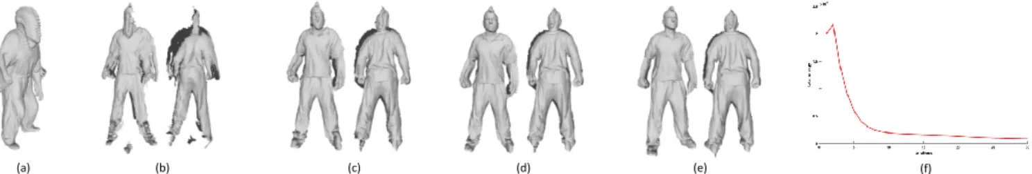
Fig. 6. Iterative results of our method. (a) initial 37 partial scans, (b) registration result after 1 iteration, (c) registration result after 10 iterations, (d) registration result after 20 iterations, (e) registration result after 30 iterations, and (f) total energy vs. the number of iterations.
vertices. Then, we find the corresponding points between neighboring scans using the approach [45]. The method is intrinsic and works well even for partial scans with large deformation. The iterative results of our method are shown in Figs. 6(a-e). Fig. 6(f) demonstrates that the total energy reduces steadily over iterations.
We apply our multi-resolution global registration to the set of models from coarse to fine. In Fig. 7(A), we show four partial scans and the deformed scans after registration using our method and alternative methods. It can be seen that the method [43] has a serious shrinkage problem and a similar phenomenon happens to the method [44] although to a lesser extent. Our method produces the best registration result. Fig. 8 and Fig. 9 illustrate the results when scans are accumulated gradually, using the first 4 scans, the first 20 scans, and all the scans for registration, compared with four state-of-the-art methods. We also use standard Poisson reconstruction [50] to obtain watertight meshes. Because the L0 method [3] requires
a template mesh for tracking, we choose a complete mesh from the original dataset as the template mesh and register this mesh to the partial meshes. We can see that the L0 method [3] has wrong estimation for the head and dress, and the PR-GLS method [4] has misalignment for the back. The shrinkage problem becomes more and more severe for L21 method [43] in arms and legs. The results of L11 method [44] have clearly visible misalignment in the results of registration and even after Poisson reconstruction, especially in the arms, which are resulted from the accumulation of registration errors. Compared with these methods, the results of our method are smoother and better aligned. By using global registration, our method does not suffer from error accumulation and the use of ARAP constraint avoids shrinking. Our results are better than alternative methods, even with only the first four views. The quantitative evaluation is given in Table II. Our method has the smallest error. The running times of L0 [3], PR-GLS [4], L21 [43], L11 [44], and our method are 20min14s, 60min45s,
Fig. 7. Comparison of results on datasets: (A)Bouncing, (B)Wavingand (C)Flying: (a) original partial scans, (b) the results of [43], (c) the results of [44] and (d) the results of our method.
7min56s, 19min30s, 180min55s, respectively. The experiments were carried out on a desktop PC with an i7 3.4-GHz CPU and 8-GB RAM. Our method is currently implemented using unoptimized MATLAB code.
To evaluate the performance for correspondences with par-tially incorrect matchings, we obtain two thirds of corre-spondences using diffusion pruning [45] and the remaining one third using local geometric feature matching based on SHOT signatures [51]. The majority of correspondences from the former are correct while many correspondences from the latter are incorrect due to the ambiguity of local features. One example of correspondences for two partial meshes is shown in Fig. 10(a), and final reconstruction results are shown in Figs. 10(b-d). Wrong correspondences are marked as red. It can be seen that our method is robust with respect to incorrect correspondences. Thanks to the regularization terms in our en-ergy function, in particular the transformation smoothness term and the as-rigid-as-possible term, incorrect correspondences which are likely to be substantially different from their neigh-boring correspondences, are substantially down-weighted, due to large regularization costs if local transformations were to follow them.
To evaluate the robustness of our method, we also experi-ment on the dataset polluted by dense noise and sparse outliers with the same approach as mentioned in Section V-A. Fig. 11 and Fig. 12 show our results compared with the other methods, and the corresponding distance errors are shown in Table II. The results show that our method is more robust to noise and outliers than the alternative methods.
TABLE II
QUANTITATIVE EVALUATION FOR PARTIAL DATASETS(CM). Method Sambaclean Bouncingclean Bouncingnoise Bouncingoutlier
L0 [3] 0.6318 1.0042 1.0437 1.0145 PR-GLS [4] 1.8008 1.6973 1.7556 2.1227 L21 [43] 1.2959 1.4986 1.5575 1.5417 L11 [44] 0.4910 0.9887 1.0158 1.0225
Ours 0.2508 0.7186 0.9849 0.9506
C. Results on Real Scans
We now test our method on real scans, which are very challenging, because they have much noise and a large num-ber of outliers. Here, we create two datasets scanned using a Kinect: Waving and Flying datasets. The Waving dataset involves large deformations which allows the hands and feet to wave forward and backward. It contains 30 scans with about 9,000-14,000 vertices for each partial scan. Sample partial models of Waving are shown in Fig. 5(b). We obtain the low-resolution models by subsampling with 1/10of vertices, similar to the clean datasets, and compare our method with the pairwise registration methods [43], [44] in Fig. 7(B). Similarly, we can see that the method [43] produces highly distorted results and the results of method [44] also contain misalignment. Fig. 13 illustrates the results when scans are accumulated gradually. Since no ground truth data is available, it is not possible to measure the errors quantitatively. However, from visual inspection, it is clear that our global registration method produces superior results. The results of [43] (top row) not only have serious shrinkage but also become more
(a) (b) (c) (d) (e)
0 6.6cm
1.0
Fig. 8. Comparative results using gradually accumulated scans on the partial datasetBouncing. Top row: L0 [3], second row: PR-GLS [4], third row: L21 [43], fourth row: L11 [44], and bottom row: our method. (a): the results of scans 1-4, (b) the results of scans 1-20, (c) the results of all the scans, (d) Poisson reconstruction results based on (c) (the top row shows the template mesh), (e) corresponding color-coded error distributions.
and more flat. With the accumulation of registration errors, the misalignment problem for method [44] also becomes unacceptable, especially in the head and arms. Our method generates significantly better results, including the head and arms.
In order to show the robustness and effectiveness of our method, for the Flying dataset, we just use 15 partial scans with dramatic deformations between scans which allow the arms to wave up and down. Sample partial models of Flying
are shown in Fig. 5(c). As shown in Fig. 7(C), there are serious distortions in the results of method [43], and the transformed scans become more flat. The misalignment of method [44] is also apparent. On the contrary, the results of our method have no such problems. Fig. 14 gives the results when scans
are accumulated gradually. The results of method [43] have a serious shrinkage problem and the misalignment problem for method [44] also becomes unacceptable. Our method has better registration results and the reconstructed complete model is accurate and watertight.
VI. CONCLUSION
This paper proposes a novel global sparse non-rigid align-ment method which registers a sequence of scans with dra-matic deformations simultaneously to reconstruct a complete object with a single RGB-D camera. We formulate the energy function with dual sparsity on both data term and smooth term, along with the local rigidity constraint and the ARAP (as-rigid-as-possible) constraint. It is solved by the alternating direction
(a) (b) (c) (d) (e)
0 10cm
1.5
Fig. 9. Comparative results using gradually accumulated scans on the partial datasetSamba. Top row: L0 [3], second row: PR-GLS [4], third row: L21 [43], fourth row: L11 [44], and bottom row: our method. (a): the results of scans 1-4, (b) the results of scans 1-20, (c) the results of all the scans, (d) Poisson reconstruction results based on (c) (the top row shows the template mesh), (e) corresponding color-coded error distributions.
(b) (c) (d)
0 6.6 cm 1.0
(a)
Fig. 10. Comparison results onBouncingdataset with partially incorrect correspondences: (a) part of correspondences for two scans, (b) registration result of all the scans, (c) Poisson reconstruction result, (d) corresponding color-coded error distributions.
method under the augmented Lagrangian multiplier (ADM-ALM) framework which has exact solutions and guaranteed convergence. Experimental results on public datasets and real scanned datasets show that our method is effective and robust for challenging deformations such as large-scale movement of
arms and legs, as well as noise and outliers. In addition, our method allows fewer partial scans to reconstruct a full object. Our method also has some limitations. First, although our method can handle a wider range of deformations, it becomes more difficult with very few scans, such as the example shown
(a) (b) (c) (d) (e)
0 6.6cm
1.0
Fig. 11. Comparative results using gradually accumulated scans on the partial datasetBouncingwith noise (σ = 0.1l). Top row: L0 [3], second row: PR-GLS [4], third row: L21 [43], fourth row: L11 [44], and bottom row: our method. (a): the results of scans 1-4, (b) the results of scans 1-20, (c) the results of all the scans, (d) Poisson reconstruction results based on (c) (the top row shows the template mesh), (e) corresponding color-coded error distributions.
in Fig. 14, since neighboring scans have less overlap. Not all the partial scans are well aligned such as the arms, although the reconstructed complete model removes most artifacts. Second, our current formulation only considers the registration errors of neighboring scans while other scans that have overlap with the current scan will also help for accurate registration. Third, the computation complexity is a little high due to the global formulation. In the future, we will investigate more robust schemes by exploiting potential overlaps between non-adjacent scans and speed up the algorithm using GPU.
REFERENCES
[1] K. Wang, G. Zhang, and S. Xia, “Templateless non-rigid reconstruction and motion tracking with a single RGB-D camera,”IEEE Transactions on Image Processing, vol. 26, no. 12, pp. 5966–5979, 2017.
[2] W. Huang, X. Cao, K. Lu, Q. Dai, and A. C. Bovik, “Toward naturalistic 2D-to-3D conversion,”IEEE Transactions on Image Processing, vol. 24, no. 2, pp. 724–733, 2015.
[3] K. Guo, F. Xu, Y. Wang, Y. Liu, and Q. Dai, “Robust non-rigid motion tracking and surface reconstruction using L0 regularization,” in IEEE International Conference on Computer Vision, 2015, pp. 3083–3091. [4] J. Ma, J. Zhao, and A. L. Yuille, “Non-rigid point set registration by
preserving global and local structures,” IEEE Transactions on Image Processing, vol. 25, no. 1, pp. 53–64, 2016.
[5] J. Lei, C. Zhang, Y. Fang, Z. Gu, N. Ling, and C. Hou, “Depth sensation enhancement for multiple virtual view rendering,”IEEE Transactions on Multimedia, vol. 17, no. 4, pp. 457–469, April 2015.
[6] J. Lei, J. Liu, H. Zhang, Z. Gu, N. Ling, and C. Hou, “Motion and structure information based adaptive weighted depth video estimation,”
IEEE Transactions on Broadcasting, vol. 61, no. 3, pp. 416–424, Sep. 2015.
[7] R. A. Newcombeet al., “KinectFusion: Real-time dense surface mapping and tracking,” inIEEE ISMAR, 2011, pp. 127–136.
[8] J. Starck, A. Maki, S. Nobuhara, A. Hilton, and T. Matsuyama, “The multiple-camera 3-D production studio,”IEEE Transactions on Circuits and Systems for Video Technology, vol. 19, no. 6, pp. 856–869, 2009.
(a) (b) (c) (d) (e)
0 6.6cm
1.0
Fig. 12. Comparative results using gradually accumulated scans on the partial datasetBouncingwith 10%outliers. Top row: L0 [3], second row: PR-GLS [4], third row: L21 [43], fourth row: L11 [44], and bottom row: our method. (a): the results of scans 1-4, (b) the results of scans 1-20, (c) the results of all the scans, (d) Poisson reconstruction results based on (c) (the top row shows the template mesh), (e) corresponding color-coded error distributions.
[9] E. De Aguiar, C. Stoll, C. Theobalt, N. Ahmed, H. P. Seidel, and S. Thrun, “Performance capture from sparse multi-view video,” inACM SIGGRAPH, 2008, p. 98.
[10] J. Tong, J. Zhou, L. Liu, Z. Pan, and H. Yan, “Scanning 3D full human bodies using Kinects,”IEEE Transactions on Visualization and Computer Graphics, vol. 18, no. 4, pp. 643–50, 2012.
[11] G. Ye, Y. Liu, N. Hasler, X. Ji, Q. Dai, and C. Theobalt, “Performance capture of interacting characters with handheld kinects,” inEuropean Conference on Computer Vision, 2012, pp. 828–841.
[12] M. Dou, H. Fuchs, and J. M. Frahm, “Scanning and tracking dynamic objects with commodity depth cameras,” inIEEE ISMAR, 2013, pp. 99–106.
[13] M. Zollh¨oferet al., “Real-time non-rigid reconstruction using an RGB-D camera,”ACM Transactions on Graphics, vol. 33, no. 4, pp. 1–12, 2014.
[14] Q. Zhang, B. Fu, M. Ye, and R. Yang, “Quality dynamic human body modeling using a single low-cost depth camera,” inIEEE Conference on Computer Vision and Pattern Recognition, 2014, pp. 676–683. [15] X. Zhou, M. Zhu, S. Leonardos, and K. Daniilidis, “Sparse
represen-tation for 3D shape estimation: A convex relaxation approach,”IEEE Transactions on Pattern Analysis and Machine Intelligence, vol. 39,
no. 8, pp. 1648–1661, 2017.
[16] K. Li, J. Yang, and J. Jiang, “Nonrigid structure from motion via sparse representation,”IEEE Transactions on Cybernetics, vol. 45, no. 8, pp. 1401–1413, 2015.
[17] P. F. U. Gotardo and A. M. Martinez, “Computing smooth time-trajectories for camera and deformable shape in structure from motion with occlusion,”IEEE Transactions on Pattern Analysis and Machine Intelligence, vol. 33, no. 10, pp. 2051–2065, 2011.
[18] M. Dou, P. Davidson, S. R. Fanello, S. Khamis, A. Kowdle, C. Rhe-mann, V. Tankovich, and S. Izadi, “Motion2fusion: real-time volumetric performance capture,”ACM Transactions on Graphics, vol. 36, no. 6, p. 246, 2017.
[19] M. Innmann, M. Zollhfer, M. Niener, C. Theobalt, and M. Stamminger, “VolumeDeform: Real-time volumetric non-rigid reconstruction,” in
European Conference on Computer Vision, 2016, pp. 362–379. [20] R. A. Newcombe, D. Fox, and S. M. Seitz, “DynamicFusion:
Re-construction and tracking of non-rigid scenes in real-time,” in IEEE Conference on Computer Vision and Pattern Recognition, 2015, pp. 343– 352.
[21] D. Guo, K. Li, Y.-K. Lai, and J. Yang, “Global alignment for deformable objects captured by a single RGB-D camera,” in IEEE International
(a) (b) (c) (d)
Fig. 13. Comparative results with scans accumulated gradually on the scannedWavingdataset. Top row: [43], middle row: [44], bottom row: our method. (a): The results of scans 1-12, (b): the results of scans 1-20, (c) the results of all the scans, (d) the Poisson reconstruction results for (c).
(a) (b) (c) (d)
Fig. 14. Comparative results with scans accumulated gradually on theFlyingdataset. Top row: [43], middle row: [44], bottom row: our method; (a): The results of scans 1-6, (b): the results of scans 1-10, (c) the results of all the scans, (d) the Poisson reconstruction results for (c).
Conference on Multimedia and Expo, 2017.
[22] D. Vlasic, I. Baran, W. Matusik, and J. Popovi´c, “Articulated mesh animation from multi-view silhouettes,”ACM Transactions on Graphics, vol. 27, no. 3, p. 97, 2008.
[23] J. Gall, C. Stoll, E. D. Aguiar, C. Theobalt, B. Rosenhahn, and H. P. Seidel, “Motion capture using joint skeleton tracking and surface estima-tion,” inIEEE Conference on Computer Vision and Pattern Recognition,
2009, pp. 1746–1753.
[24] K. Li, Q. Dai, and W. Xu, “Markerless shape and motion capture from multi-view video sequences,”IEEE Transactions on Circuits and systems for Video Technology, vol. 21, no. 3, pp. 320–334, 2011.
[25] A. Collet, M. Chuang, P. Sweeney, D. Gillett, D. Evseev, D. Calabrese, H. Hoppe, A. Kirk, and S. Sullivan, “High-quality streamable free-viewpoint video,”ACM Transactions on Graphics, vol. 34, no. 4, pp.
1–13, 2015.
[26] S. Lin, Y. Chen, Y.-K. Lai, R. R. Martin, and Z.-Q. Cheng, “Fast capture of textured full-body avatar with RGB-D cameras,”The Visual Computer, vol. 32, no. 6–8, pp. 681–691, 2016.
[27] M. Dou, S. Khamis, Y. Degtyarev, P. Davidson, S. R. Fanello, A. Kow-dle, S. O. Escolano, C. Rhemann, D. Kim, and J. Taylor, “Fusion4D: real-time performance capture of challenging scenes,”ACM Transactions on Graphics, vol. 35, no. 4, p. 114, 2016.
[28] A. Weiss, D. Hirshberg, and M. J. Black, “Home 3D body scans from noisy image and range data,” in IEEE International Conference on Computer Vision, 2011, pp. 1951–1958.
[29] Y. Cui, W. Chang, T. N¨oll, and D. Stricker, “KinectAvatar: Fully automatic body capture using a single kinect,” in ACCV Workshops, 2012, pp. 133–147.
[30] H. Li, E. Vouga, A. Gudym, L. Luo, J. T. Barron, and G. Gusev, “3D self-portraits,”ACM Transactions on Graphics, vol. 32, no. 6, pp. 2504– 2507, 2013.
[31] M. Dou, J. Taylor, H. Fuchs, A. Fitzgibbon, and S. Izadi, “3D scanning deformable objects with a single RGBD sensor,” inIEEE Conference on Computer Vision and Pattern Recognition, 2015, pp. 493–501. [32] D. Vlasic, P. Peers, I. Baran, P. Debevec, S. Rusinkiewicz, and W.
Ma-tusik, “Dynamic shape capture using multi-view photometric stereo,”
ACM Transactions on Graphics, vol. 28, no. 5, pp. 174:1–11, 2009. [33] H. Li, B. Adams, L. J. Guibas, and M. Pauly, “Robust single-view
geometry and motion reconstruction,”ACM Transactions on Graphics, vol. 28, no. 5, p. 175, 2009.
[34] M. Liao, Q. Zhang, H. Wang, and R. Yang, “Modeling deformable objects from a single depth camera,” inIEEE International Conference on Computer Vision, 2009, pp. 167–174.
[35] G. K. Tam et al., “Registration of 3D point clouds and meshes: a survey from rigid to nonrigid,”IEEE Transations on Visualization and Computer Graphics, vol. 19, no. 7, pp. 1199–1217, 2013.
[36] H. Lei, G. Jiang, and L. Quan, “Fast descriptors and correspondence propagation for robust global point cloud registration,”IEEE Transac-tions on Image Processing, 2017.
[37] S. Bouaziz, A. Tagliasacchi, and M. Pauly, “Sparse iterative closest point,”Computer Graphics Forum, vol. 32, no. 5, pp. 113–123, 2013. [38] M. Ruhnke, R. Kummerle, G. Grisetti, and W. Burgard, “Highly accurate
3D surface models by sparse surface adjustment,” inIEEE International Conference on Robotics and Automation, 2012, pp. 751–757. [39] S. Bouaziz and M. Pauly, “Dynamic 2D/3D registration for the Kinect,”
inACM SIGGRAPH Courses, 2013, pp. 21:1–21:14.
[40] J. Ma, W. Qiu, J. Zhao, Y. Ma, A. L. Yuille, and Z. Tu, “Robust l2e esti-mation of transforesti-mation for non-rigid registration.”IEEE Transactions on Signal Processing, vol. 63, no. 5, pp. 1115–1129, 2015.
[41] J. Ma, J. Zhao, J. Tian, A. L. Yuille, and Z. Tu, “Robust point matching via vector field consensus.”IEEE Transactions on Image Processing, vol. 23, no. 4, pp. 1706–1721, 2014.
[42] J. Ma, H. Zhou, J. Zhao, Y. Gao, J. Jiang, and J. Tian, “Robust feature matching for remote sensing image registration via locally linear transforming,”IEEE Transactions on Geoscience and Remote Sensing, vol. 53, no. 12, pp. 6469–6481, 2015.
[43] J. Yang, K. Li, K. Li, and Y.-K. Lai, “Sparse non-rigid registration of 3D shapes,”Comp. Graph. Forum, vol. 34, no. 5, pp. 89–99, 2015. [44] J. Yang, K. Li, Y.-K. Lai, and D. Guo, “Robust non-rigid registration
with reweighted position and transformation sparsity,” IEEE Transac-tions on Visualization and Computer Graphics, 2018.
[45] G. K. Tam, R. R. Martin, P. L. Rosin, and Y.-K. Lai, “Diffusion pruning for rapidly and robustly selecting global correspondences using local isometry.”ACM Transactions on Graphics, vol. 33, no. 1, p. 4, 2014. [46] O. Sorkine and M. Alexa, “As-rigid-as-possible surface modeling,”Proc.
Symposium on Geometry Processing, pp. 109–116, 2007.
[47] M. Garland and P. S. Heckbert, “Surface simplification using quadric error metrics,” inACM SIGGRAPH, 1997, pp. 209–216.
[48] S. Boyd, N. Parikh, E. Chu, B. Peleato, and J. Eckstein, “Distributed optimization and statistical learning via the alternating direction method of multipliers,”Foundations and TrendsR in Machine Learning, vol. 3, no. 1, pp. 1–122, 2011.
[49] P. Cignoni, C. Rocchini, and R. Scopigno, “METRO: Measuring error on simplified surfaces,”Computer Graphics Forum, vol. 17, no. 2, pp. 167–174, 1998.
[50] M. Kazhdan and H. Hoppe, “Screened poisson surface reconstruction,”
ACM Transactions on Graphics, vol. 32, no. 3, p. 29, 2013.
[51] S. Salti, F. Tombari, and L. Di Stefano, “SHOT: unique signatures of histograms for surface and texture description,”Computer Vision and Image Understanding, vol. 125, pp. 251–264, 2014.
Jingyu Yang(M’10-SM’17) received the B.E. de-gree from Beijing University of Posts and Telecom-munications, Beijing, China, in 2003, and Ph.D. (Hons.) degree from Tsinghua University, Beijing, in 2009. He has been a Faculty Member with Tianjin University, China, since 2009, where he is currently a Professor with the School of Electrical and Information Engineering. He was with Microsoft Research Asia (MSRA) in 2011, and the Signal Pro-cessing Laboratory, EPFL, Lausanne, Switzerland, in 2012, and from 2014 to 2015. His research interests include image/video processing, 3D imaging, and computer vision. He has authored or co-authored over 80 high quality research papers. As a co-author, he got the best 10% paper award in IEEE VCIP 2016 and the Platinum Best Paper award in IEEE ICME 2017. He served as special session chair in VCIP 2016 and area chair in ICIP 2017.
Daoliang Guo received the B.E. degree from the School of Electronic Information Engineering, An-hui University in 2015, and the M.E. degree at the School of Electrical and Information Engineering, Tianjin University in 2018. He is currently serving for the AILab of Netease Games in Hangzhou, China. His research interests include 3D registration, reconstruction and Animation.
Kun Lireceived the B.E. degree from Beijing Uni-versity of Posts and Telecommunications, Beijing, China, in 2006, and the master and Ph.D. degrees from Tsinghua University, Beijing, in 2011. She visited ´Ecole Polytechnique F´ed´erale de Lausanne, Lausanne, Switzerland, in 2012 and from 2014 to 2015. She is currently an Associate Professor with the School of Computer Science and Technology, Tianjin University, Tianjin, China. Her research in-terests include dynamic scene 3D reconstruction and image/video processing. She was selected into Peiyang Scholar Program of Tianjin University in 2016, and got the Platinum Best Paper award in IEEE ICME 2017.
Zhenchao Wu received the B.E. degree from the School of Computer Science, Xi’an Polytechnic University, Xi’an, China, in 2017. He is currently pursuing the M.E. degree at the College of Intelli-gence and Computing, Tianjin University, Tianjin, China. His interests are mainly in 3D registration and reconstruction.
Yu-Kun Lai received his bachelor and Ph.D. de-grees in computer science from Tsinghua University in 2003 and 2008, respectively. He is currently a Reader of Visual Computing in the School of Computer Science & Informatics, Cardiff University. His research interests include computer graphics, ge-ometry processing, image processing and computer vision. He is on the editorial board of The Visual Computer.
![Fig. 4. Comparison results on the Jumping dataset with 10% outliers: (a) original complete models with outliers, (b) the results of [3], (c) the results of PR-GLS [4], (d) the results of [43], (e) the results of [44], and (f) our results.](https://thumb-us.123doks.com/thumbv2/123dok_us/9234723.2808206/8.918.119.795.843.1059/comparison-results-jumping-dataset-outliers-original-complete-outliers.webp)
![Fig. 7. Comparison of results on datasets: (A) Bouncing, (B) Waving and (C) Flying: (a) original partial scans, (b) the results of [43], (c) the results of [44]](https://thumb-us.123doks.com/thumbv2/123dok_us/9234723.2808206/10.918.78.839.78.493/comparison-results-datasets-bouncing-waving-flying-original-partial.webp)


