SFB
823
Subsampling for general
statistics under long range
dependence
Discussion Paper
Annika Betken, Martin Wendler
Subsampling for General Statistics
under Long Range Dependence
Annika Betken∗, Martin Wendler
Ruhr-Universit¨at Bochum e-mail:[email protected]
Ernst-Moritz-Arndt-Universit¨at Greifswald e-mail:[email protected]
Abstract: In the statistical inference for long range dependent time series, the shape of the limit distribution typically dependents on unknown param-eters. Therefore, we propose to use subsampling. We show the validity of subsampling for general statistics and long range dependent subordinated Gaussian processes, which satisfy mild regularity conditions. We apply our method to a self-normalized change-point test statistic and investigate the finite sample properties in a simulation study.
MSC 2010 subject classifications:Primary 60G15, 62G09; secondary 60G22.
Keywords and phrases:Subsampling, Gaussian Processes, Long Range Dependence, Change Point Test.
1. Introduction
1.1. Long Range Dependence
While most statistical research is done for independent data or short memory time series, in many applications there are also time series with long memory in the sense of slowly decaying correlations: in hydrology (starting with the work of Hurst [23]), in finance (e.g. Lo [30]), in the analysis of network traffic (e.g. Leland, Taqqu, Willinger and Wilson [29]) and many more fields of research.
As model of dependent time series, we will consider subordinated Gaussian processes: Let (ξn)n∈N be a stationary sequence of centered Gaussian variables
with Var(ξn) = 1 and covariance function γsatisfying
γ(k) := Cov(ξ1, ξk+1) =k−DLγ(k), (1)
for a D > 0 and a slowly varying function Lγ. If D < 1, then the spectral
densityf of (ξn)n∈Nis not continuous, but has a pole at 0. The spectral density
has the form
f(x) =|x|D−1L
f(x)
for a functionLf, which is slowly varying at the origin (see Proposition 1.1.14
in Pipiras and Taqqu [35]).
∗supported by Collaborative Research Center SFB 823 and by the German Academic
Foundation
Furthermore, letG:R→Rbe a measurable function such that E[G2( 1)]<
∞. The stochastic process (Xn)n∈N given by
Xn :=G(ξn)
is called long range dependent ifP∞
n=0|Cov(X1, Xn+1)|=∞, and short range
dependent ifP∞
n=0|Cov(X1, Xn+1)|<∞.
In limit theorems for the partial sumSn =P n
i=1Xi, the normalization
re-quired and the shape of the limit distribution depend not only on the decay of the covariancesγ(k) ask→ ∞, but also on the function G. More precisely, Taqqu [43] and Dobruhsin, Major [18] independently proved that
1 Lγ(n)r/2nH n X i=1 (Xi−E[Xi]) D −→C(r, H)grZr,H(1),
if the Hurst parameterH := max{1−rD
2 , 1
2}is greater than 1
2.ris the Hermite
rank of the functionG,gris the first non-zero coefficient in the expansion ofGas
a sum of Hermite polynomials andZr,His a Hermite process. For more details on
Hermite polynomials and limit theorems for subordinated Gaussian processes, we recommend the book of Pipiras and Taqqu [35]. In this case (rD < 1), the process (Xn)n∈Nis long range dependent, as the covariances are not summable.
Note that the limiting random variableC(r, H)Zr,H(1) is Gaussian only if the
Hermite rankr= 1.
If rD = 1, the process (Xn)n∈N might be short or long range dependent
according to the slowly varying function Lγ. If rD > 1, the process is short
range dependent. In this case, the partial sumPn
i=1(Xi−E[Xi]) has (with the
proper normalization) always a Gaussian limit.
There are other models for long-memory processes: Fractionally integrated autoregressive moving average processes can show long range dependence, see Granger and Joyeux [20]. General linear processes with slowly decaying coeffi-cients were studied by Surgailis [42].
1.2. Subsampling
In practical applications, the parametersD,rand the slowly varying functionLγ
are unknown and thus the scaling needed in the limit theorems and the shape of the asymptotic distribution are not known, either. That makes it difficult to use the asymptotic distribution for statistical inference. The situation gets even more complicated if one is not interested in partial sums, but in nonlinear statistical functionals. For example,U-statistics can have a linear combination of random variables related to different Hermite ranks as a limit, see Beutner and Z¨ahle [10]. Self-normalized statistics typically converge to quotients of two random variables (e.g. McElroy and Politis [33]). The change-point test proposed by Berkes, Horv´ath, Kokoszka and Shao [8] converges under the alternative hypothesis to a supremum of a fractional Brownian bridge.
To overcome the problem of the unkown shape of the limit distribution and to avoid the estimation of nuisance parameters, one would like to use nonpara-metric methods. However, Lahiri [28] has shown that the popular moving block bootstrap might fail under long range dependence. Another nonparametric ap-proach is subsampling (also called sampling window method), first studied by Politis and Romano [36], Hall and Jing [21], and Sherman and Carlstein [40]. The idea is the following: LetTn =Tn(X1, . . . , Xn) be a series of statistics
con-verging in distribution to a random variable T, but as we typically only have one sample, we observe only one realization of Tn and can not estimate the
distribution ofTn. But ifl=ln is a sequence withln→ ∞andln =o(n), then
Tlalso converges in distribution toT and we have multiple (though dependent)
realizationsTl(X1, . . . , Xl), Tl(X2, . . . , Xl+1),...,Tl(Xn−l+1, . . . , Xn), which we
can use to calculate the empirical distribution function. The validity of subsampling for the sample mean ¯X = 1
n
Pn
i=1Xiunder long
range dependence has been investigated in the literature starting with Hall, Jing and Lahiri [22] for subordinated Gaussian processes. Nordman and Lahiri [34] and Zhang, Ho, Wendler, Wu [47] studied linear processes with slowly decaying coefficients. An alternative proof in the case of Gaussian processes can be found in the book of Beran, Feng, Ghosh, Kulik [7].
It was noted by Fan [19] that the proof of Hall et al. [22] can be easily generalized to other statistics than the sample mean. However, the assumptions on the Gaussian process are restrictive (see also McElroy and Politis [33]). Their conditions imply that the sequence (ξn)n∈N is completely regular, which might
hold for some special cases (see Ibragimov and Rozanov [24]), but excludes many examples:
Example 1 (Fractional Gaussian Noise). Let (BH(t))t∈[0,∞) be a fractional
Brownian motion, i.e. a centered, self-similar Gaussian process with covariance function
E [BH(t)BH(s)] =
1 2 t
2H+s2H− |t−s|2H
for someH ∈(12,1). Then (ξn)n∈N given byξn=BH(n)−BH(n−1) is called
fractional Gaussian noise. By self-similarity, we have
corr n X i=1 ξi, 3n X j=2n+1 ξj = corr (BH(n), BH(3n)−BH(2n)) = corr (BH(1), BH(3)−BH(2)).
So the correlations of linear combinations of observations in the past and future do not vanish if the gap between past and future grows and thus fractional Gaussian noise is not completely regular.
Jach, McElroy, Politis [25] provided a more general result on the validity of subsampling. They assume that the functionGhas Hermite rank 1, that Gis invertible and Lipschitz-continuous and that the process (ξn)n∈N has a causal
These assumptions are difficult to check in practice. Moreover, although not ex-plicitly stated in their Theorem 4, the statisticTnhas to be Lipschitz-continuous
(uniformly inn), which is not satisfied by many robust estimators (see Section 3 for an example).
The main aim of this paper is to establish the validity of the subsampling method for general statisticsTn without any assumptions on the continuity of
the statistic, on the function G and only mild assumptions on the Gaussian process (ξn)n∈N. We will give our main theorem in the next section. In Section
3, we will apply our theorem to a self-normalized, robust change-point statistic. The finite sample properties of this test will be investigated in Section 4. Finally, the proof of the main result and the lemmas needed can be found in Section 5.
2. Main Results
2.1. Statement of the Theorem
For a statistic Tn = Tn(X1, . . . , Xn), the subsampling estimator ˆFl,n of the
distribution functionFTn withFTn(t) = P(Tn ≤t) is defined in the following
way: Let fort∈R ˆ Fl,n(t) = 1 n−l+ 1 n−l+1 X j=1 1{Tl(Xi,...,Xi+l−1)≤t}.
Our first assumption guarantees the convergence of the distribution function of
Tn:
Assumption 1. (Xn)n∈N is a stochastic process and (Tn)n∈N is a sequence
of statistics, such that Tn → T in distribution for a random variable T with
distribution functionFT.
This is a standard assumption for subsampling, see for example Politis and Romano [36]. If the distribution does not converge, we can not expect the dis-tribution ofTlto be close to the distribution ofTn.
Next, we will formulate our conditions on the sequence (Xn)n∈N of random
variables:
Assumption 2. Xn = G(ξn) for a measurable function G and a stationary,
Gaussian process(ξn)n∈N with covariance function
γ(k) := Cov(ξ1, ξ1+k) =k−DLγ(k)
such that the following conditions hold:
1. D∈(0,1]andLγ is a slowly varying function with
max ˜ k∈{k+1,...,k+2l0−1} Lγ(k)−Lγ(˜k) ≤K l0 kmin{Lγ(k),1}
2. (ξn)n∈N has a spectral density f with f(x) = |x|D−1Lf(x) for a slowly
varying functionLf which is bounded away from0 on [0, π].
While we have some regularity conditions on the underlying Gaussian process (ξn)n∈N, note that we do not have any conditions on the function G, no finite
moments or continuity are required, which will make our results applicable for heavy-tailed random variables and robust test statistics. We will show that As-sumption 2 holds for some standard examples of long range dependent Gaussian processes in the next subsection.
Furthermore, we need a restriction on the growth rate of the block lengthl:
Assumption 3. Let(ln)n∈N be a nondecreasing sequence of integers such that
l=ln→ ∞as n→ ∞andln=O n(1+D)/2−
for an >0.
If the dependence of the underlying process (ξn)n∈N gets stronger, the range
of possible values for l gets smaller. A popular choice for the block length is
l ≈C√n(see for example Hall et al. [22]), which is allowed for allD ∈ (0,1]. Now we can state our main result:
Theorem 1. Under the Assumptions 1, 2 and 3 for all points of continuity t
ofFT, we have FTn(t)−Fˆl,n(t) P −→0. IfFT is continuous, then sup t∈R FTn(t)−Fˆl,n(t) P −→0.
So we have a consistent estimator for the distribution function ofTn and it
is possible to build tests and confidence intervals based on this estimator. IfD >1, then the process (ξn)n∈N is strongly mixing by Theorem 9.8 in the
book of Bradley [13] and the statements of our theorem hold by Corollary 3.2 in Politis and Romano [36] for any blocklengthlsatisfyingl→ ∞andl=o(n).
2.2. Examples for our Assumptions
We will now give two examples of Gaussian processes satisfying Assumption 2:
Example 2 (Fractional Gaussian Noise). Fractional Gaussian Noise (ξn)n∈N
with Hurst parameterHas introduced in Example 1 has the covariance function
γ(k) = 1
2 |k−1|
2H−2|k|2H+|k+ 1|2H
=H(2H−1) k−D+h(k)k−D−1 forD= 2−2H and a functionhbounded by a constantM <∞, which can be easily seen by means of a Taylor expansion. SoLγ(k) =H(2H−1)(1 +h(k)/k)
and for all ˜k≥k
Lγ(k)−Lγ(˜k) ≤H(2H−1) h(k) k − h(˜k) ˜ k ≤H(2H−1)M k =:K 1 k
implying Part 1 of Assumption 2. For the second part, note that spectral density
f of fractional Gaussian noise is given by
f(λ) =C(H)(1−cos(λ)) ∞ X k=−∞ |x+ 2kπ|D−3 =λD−1C(H)1−cos(λ) λ2 P∞ k=−∞|λ+ 2kπ| D−3 λD−3
see Sinai [41]. The slowly varying function
Lf(λ) =C(H) 1−cos(λ) λ2 P∞ k=−∞|λ+ 2kπ| D−3 λD−3
is bounded away from 0 because this obviously holds for the first factor (1−
cos(λ))/λ2 and P∞ k=−∞|λ+ 2kπ| D−3 λD−3 ≥ |λ+ 20π|D−3 λD−3 = 1.
Example 3 (Gaussian FARIMA processes). Let (εn)n∈Z be Gaussian white
noise with variance σ2 = Var(ε0). Then for a d ∈ (0,1/2), a FARIMA(0,d,0)
process (ξn)n∈N is given by ξn= ∞ X j=0 Γ(j+d) Γ(j+ 1)Γ(d)εn−j.
According to Pipiras and Taqqu [35], Section 1.3, it has the specral density
f(λ) = σ 2 2π|1−e −iλ |−2d=|λ|D−1σ 2 2π |λ| |1−e−iλ| 1−D
withD= 1−2d∈(0,1). As|1−e−iλ| ≤λ, part 2 of Assumption 2 holds. For part 1, we have by Corollary 1.3.4 of [35] that
γ(k) =σ2 Γ(1−2d)
Γ(1−d)Γ(d)
Γ(k+d) Γ(k−d+ 1). Recall that by the Stirling formula Γ(x) = 2π
x 1/2 x e x 1 +O(x−1) and con-sequently γ(k) =σ2 Γ(1−2d) Γ(1−d)Γ(d)e −2d+1k2d−1k+d k k+d k k−d+ 1 k−d+1 1 +O 1 k .
Using a Taylor expansion of (k+d) log(k+d)−log(k)
+ (k−d+ 1) log(k)−
log(k−d+ 1), it easily follows that
γ(k) =k−DLγ(k)
withLγ(k) =C+O(1/k) for a constant C. Part 1 of Assumption 2 follows in
It would be interesting to know if the subsampling for general statistics is consistent for long range dependent linear proceseses without the assumption of gaussianity, but this seems to be a very hard problem and goes beyond the scope of this paper.
3. Application
3.1. Robust, Self-Normalized Change-Point Test
In this paper, the main motivation for considering subsampling procedures in order to approximate the distribution of test statistics consists in avoiding the choice of unknown parameters. As an example we will consider a self-normalized test statistic that can be applied to detect changes in the mean of long range dependent and heavy-tailed time series.
Given observationsX1, . . . , Xn with Xi=G(ξi) +µi we are concerned with
a decision on the change-point problem
H:µ1=. . .=µn
against
A:µ1=. . .=µk6=µk+1=. . .=µn for somek∈ {1, . . . , n−1}.
Under the hypothesisH we assume that the data generating process (Xn)n∈N is stationary, while under the alternative A there is a change in location at an unknown point in time. This problem has been widely studied: Cs¨org˝o and Horv´ath [15] give an overview of parametric and non-parametric methods that can be applied in order to detect change-points in independent data.
Many commonly used testing procedures are based on Cusum (cumulated sum) test statistics, but when applied to data sets generated by long range dependent processes, these change-point tests often falsely reject the hypothesis of no change in the mean (see also Baek and Pipiras [4]). Furthermore, the performance of Cusum-like change-point tests is sensitive to outliers in the data. In contrast, testing procedures that are based on rank statistics have the advantage of not being sensitive to outliers in the data. These were introduced by Antoch et al. [3] for detecting changes in the distribution function of independent random variables. Wilcoxon type rank tests have been studied by Wang [45] in the presence of linear long memory time series and by Dehling, Rooch and Taqqu [16] for subordinated Gaussian sequences.
Note that the normalization of the Wilcoxon change-point test statistic as proposed in [16] depends on the slowly varying functionLγ, the LRD parameter
D and the Hermite rank r of the class of functions 1{Xi≤x}−F(x), x ∈ R.
Althoughr= 1 is assumed in many cases and while there are well-tried methods to estimateD, estimatingLγ does not seem to be an easy task. For this reason,
the Wilcoxon change-point test does not seem to be suitable for application to real data.
So as to avoid these issues Betken [9] proposes an alternative normalization for the Wilcoxon change-point test. This normalization approach has originally been established by Lobato [31] for decision on the hypothesis that a short range dependent stochastic process is uncorrelated up to a lag of a certain order. In change-point analysis the normalization has recently been applied to several test statistics: Shao and Zhang [39] define a self-normalized Kolmogorov-Smirnov test statistic that serves to identify changes in the mean of short range dependent time series. Shao [38] adopted the normalization so as to define an alternative normalization for a Cusum test, which detects changes in the mean of short range dependent as well as long range dependent time series.
For the definition of the self-normalized Wilcoxon test statistic, we introduce the ranks Ri = rank(Xi) = P
n
j=11{Xj≤Xi} for i = 1, . . . , n. It seems natural
to transfer the normalization that has been used by Shao [38] on the Cusum test statistic to the ranks in order to establish a self-normalized version of the Wilcoxon test statistic, which is robust to outliers in the data. Therefore, the corresponding two-sample test statistic is defined by
Gn(k) = Pk i=1Ri−nkP n i=1Ri 1 n Pk t=1S 2 t(1, k) +n1 Pn t=k+1S 2 t(k+ 1, n) 1/2, where St(j, k) = t X h=j Rh−R¯j,k with ¯Rj,k= 1 k−j+ 1 k X t=j Rt.
The self-normalized Wilcoxon change-point test rejects the hypothesis for large values of maxk∈{bnτ1c,...,bnτ2c}|Gn(k)|, where 0< τ1 < τ2 <1. The proportion
of the data that is included in the calculation of the supremum is restricted by
τ1 and τ2. A common choice for these parameters is τ1 = 1−τ2 = 0.15; see
Andrews [2].
For long range dependent subordinated Gaussian processes (Xn)n∈N, the asymptotic distribution of the test statistic under the hypothesis H can be derived by the continuous mapping theorem (see Theorem 1 in Betken [9]):
Tn(τ1, τ2) := max k∈{bnτ1c,...,bnτ2c} |Gn(k)| ⇒ sup τ1≤λ≤τ2 |Zr(λ)−λZr(1)| Rλ 0(Zr(t)− t λZr(λ))2dt+ R1−λ 0 (Zr?(t)− t 1−λZr?(1−λ))2dt 1/2.
Here,Zris ar-th order Hermite process with Hurst parameterH := max{1− rD
2 , 1
2} and Z
?
t(r) = Zr(1)−Zr(1−t). A comparison of Tn(τ1, τ2) with the
critical values of its limit distribution still presupposes determination of these parameters, but Assumption 1 holds and we can bypass the estimation ofDand
rby applying the subsampling procedure.
Note that even under the alternativeA(change in location), we have to find the quantiles of the distribution under the hypothesis (stationarity). But as the
block lengthl is much shorter than the sample sizen, most blocks will not be contaminated by the change-point and so the distribution of the test statistic will not change. Even for blocks which cover the change, the power of the test is low (because there are onlyl observations) and thus the distribution will not change too much. The accuracy and the power of the test will be investigated by a simulation study in Section 4.
3.2. Data Examples
We will revisit some data sets which have been analyzed before in the litera-ture. We will use the self-normalized Wilcoxon change-point test combined with subsampling and compare our findings to the conclusions of other authors.
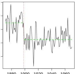
time ann ual discharge 1880 1900 1920 1940 1960 600 800 1000 1200 1400
Figure 1. The annual discharge from the Nile at Aswan in108 m3for 1871-1970. The dotted line indicates the location of the change-point; the dashed lines designate the sample means for the pre-break and post-break samples.
The plot in Figure 1 depicts the annual volume of discharge from the Nile river at Aswan in 108 m3 for the years 1871 to 1970. The data set has been analyzed for the detection of a change-point by numerous authors under differing assumptions concerning the data generating random process and by usage of diverse methods. Amongst others, Cobb [14], MacNeill, Tang and Jandhyala [32], Wu and Zhao [46] and Shao [38] provided statistical significant evidence for a decrease of the Nile’s annual discharge towards the end of the 19th century. The construction of the Aswan Low Dam between 1898 and 1902 serves as a popular explanation for an abrupt change in the data.
The value of the self-normalized Wilcoxon test statistic computed with re-spect to the data is given by Tn(τ1, τ2) = 13.48729. For a level of significance
of 5%, the self-normalized Wilcoxon change-point test rejects the hypothesis for every possible value ofH ∈ 1
2,1
. Furthermore, we approximate the dis-tribution of the self-normalized Wilcoxon test statistic by the sampling window method with block size l = b√nc. The subsampling-based test decision also indicates the existence of a change-point in the mean of the data.
In particular, previous analysis of the Nile data done by Wu and Zhao [46] and Balke [5] suggests that the change in the discharge volume occured in 1899. We applied the self-normalized Wilcoxon test and the sampling window method to the corresponding prebreak and postbreak samples. Neither of these two approaches leads to rejection of the hypothesis, so that it seems reasonable to consider both samples as stationary . At this point, it is interesting to note that, based on the whole sample, local Whittle estimation with bandwidth parameter
m =bn2/3c suggests the existence of long range dependence characterized by
an Hurst parameter ˆH = 0.962, whereas the estimates for the prebreak and postbreak samples given by ˆH1 = 0.517 and ˆH2 = 0.5, respectively, should
be considered as indication of short range dependent data. In this regard our findings support the conjecture of spurious long memory caused by a change-point and therefore coincide with the results of Shao [38].
The second data set consists of the seasonally adjusted monthly deviations of the temperature (degrees C) for the northern hemisphere during the years 1854 to 1989 from the monthly averages over the period 1950 to 1979. The data results from spatial averaging of temperatures measured over land and sea. At first sight the plot in Figure 2 may suggest an increasing trend as well as an abrupt change of the temperature deviations. Statistical evidence for a positive deterministic trend implies affirmation of the conjecture that there has been global warming during the last decades.
In scientific discourse the question of whether the Northern hemisphere tem-perature data acts as an indicator for global warming of the atmosphere is a controversial issue. Deo and Hurvich [17] provided some indication for global warming by fitting a linear trend to the data. Beran and Feng [6] considered a more general stochastic model by the assumption of so called semiparametric fractional autoregressive (SEMIFAR) processes. Their method did not deliver sufficient statistical evidence for a deterministic trend. Wang [44] applied an-other method for the detection of gradual change to the global temperature data and did not detect an increasing trend either. But he offers an alternative explanation for the occurence of trend-like behavior by pointing out that it may have been generated by stationary long range dependent processes. In contrast, it is shown in Shao [38] that the existence of a change-point in the mean yields yet another explanation for the performance of the data.
The value of the self-normalized Wilcoxon test statistic computed with re-spect to the data is given by Tn(τ1, τ2) = 18.98636. Consequently, the
self-normalized Wilcoxon change-point test would reject the hypothesis for every possible value of H ∈ 1
2,1
at a level of significance of 1%. In addition, an application of the sampling window method with respect to the self-normalized
time Nor ther n hemisphere temper ature 1860 1900 1940 1980 −1.5 −1.0 −0.5 0.0 0.5
Figure 2. Monthly temperature for the northern hemisphere for the years 1854-1989, from the data base held at the Climate Research Unit of the University of East Anglia, Norwich, England. The numbers consist of the temperature (degrees C) difference from the monthly average over the period 1950-1979. The dotted line indicates the location of the potential change-point; the dashed lines designate the sample means for the pre-break and post-break samples.
Wilcoxon test statistic yields a test decision in favor of the alternative hypothe-sis for any possible choice of the block length. All in all, both testing procedures provide strong evidence for the existence of a change in the mean.
According to Shao [38] the change-point is located around October 1924. Based on the whole sample local Whittle estimation with bandwidthm=bn2/3c
provides an estimator ˆH = 0.811. The estimated Hurst parameters for the prebreak and postbreak sample are ˆH1 = 0.597 and ˆH2 = 0.88, respectively.
Neither of both testing procedures, i.e. subsampling with respect to the self-normalized Wilcoxon test statistic and comparison of the value of Tn(τ1, τ2)
with the corresponding critical values of its limit distribution, provides evidence for another change-point in the prebreak or postbreak sample.
Therefore, it seems safe to conclude that the appearance of long memory in the postbreak sample is not caused by another change-point in the mean. The pronounced difference between the local Whittle estimators ˆH1and ˆH2suggests
a change in the dependence structure of the times series. Another explanation might be a gradual change of the temperature in the postbreak period.
In both data examples, we find that the results obtained by subsampling and obtained by parameter estimation are in good accordance with each other. The
methods take into account possible long range dependence or heavy tails, but they still can detect a change in location.
4. Simulations
We will now investigate the finite sample performance of the subsampling pro-cedure with respect to the self-normalized Wilcoxon test and with respect to the classical Wilcoxon change-point test. Moreover, we will compare these results to the performance of the tests when the test decision is based on critical values obtained from the asymptotic distribution of the test statistic.
For this purpose, we consider subordinated Gaussian time series (Xn)n∈N,
Xn=G(ξn), where (ξn)n∈Nis fractional Gaussian noise (introduced in Example 2) with Hurst parameterH ∈ {0.6,0.7,0.8,0.9} and covariance function
γ(k)∼k−D 1−D 2 (1−D) whereD= 2−2H, i.e. Lγ(k)∼ 1−D2(1−D).
Initially, we takeG(t) = t, so that (Xn)n∈N has normal marginal
distribu-tions. We also consider the transformation
G(t) = βk2 (β−1)2(β−2) −12 k(Φ(t))−1β − βk β−1
with Φ denoting the standard normal distribution function so as to generate Pareto-distributed data with parametersk, β >0 (referred to as Pareto(β,k)). In both cases the Hermite rankrof 1{G(ξi)≤x}−F(x), x∈R, equals r= 1 and
Z R J1(x)dF(x) = 1 2√π;
see Dehling, Rooch and Taqqu [16].
Under the above conditions the critical values of the asymptotic distribution of the self-normalized Wilcoxon test statistic are reported in Table 2 in Betken [9]. The limit of the Wilcoxon change-point test statistic can be found in [16], the corresponding critical values can be taken from Table 1 in [9].
The frequencies of rejections of both testing procedures are reported in Table 1 for the self-normalized Wilcoxon change-point test and in Table 2 for the classical Wilcoxon test (without self-normalization). The calculations are based on 5,000 realizations of time series with sample sizen= 300 and n= 500.
For the usual testing procedures the estimation of the Hermite rankr, the slowly varying functionLγ and the integral
R
J1(x)dF(x) is neglected. Yet, for
every simulated time series we estimate the Hurst parameter H by the local Whittle estimator ˆH proposed in K¨unsch [27]. This estimator is based on an approximation of the spectral density by the periodogram at the Fourier fre-quencies. It depends on the spectral bandwidth parameter m = m(n) which
denotes the number of Fourier frequencies used for the estimation. If the band-width m satisfies m1 + mn −→ 0 as n −→ ∞, the local Whittle estimator is a consistent estimator forH; see Robinson [37]. For convenience we always choose
m= bn2/3c in this article. The critical values corresponding to the estimated
values ofH are determined by linear interpolation.
Under the alternativeAwe analyze the power of the testing procedures (the frequency of rejection) by considering different choices for the height of the level shift (denoted byh) and the location [nτ] of the change-point. In the tables the columns that are superscribed by “h= 0” correspond to the frequency of a type 1 error, i.e. the rejection rate under the hypothesisH.
For the self-normalized Wilcoxon change-point test (based on the asymptotic distribution), the empirical size almost equals the level of significance of 5% for normally distributed data (see Table 1). The sampling window method yields a rejection rate that slightly exceeds this level. For Pareto(3, 1) time series both testing procedures lead to similar results and tend to reject the hypothesis too often when there is no change. With regard to the empirical power it is notable that for fractional Gaussian noise time series the sampling window method yields considerably better power than the test based on asymptotic critical values. If Pareto(3, 1) distributed time series are considered, the empirical power of the subsampling procedure is still better than the empirical power that results from using asymptotic critical values. However, in this case the deviation of the rejection rates is rather small. While the empirical size is not much affected by the Hurst parameterH, the empirical power is lower forH = 0.8,0.9.
Considering the classical Wilcoxon test (without self-normalization), it is no-table that for both procedures, the empirical size is in most cases not close to the nominal level of significance (5%), ranging from 1.1% to 17.5% using sub-sampling and from 2.6% to 36.0% using asymptotic critical values (see Table 2). In general, the sampling window method becomes more conservative for higher values of the Hurst parameterH, while the test based on the asymptotic distri-bution becomes more liberal. Under the alternative the usual application of the Wilcoxon test yields better power than the sampling window method, especially for high values ofH. But we emphasize that this comparison is problematic be-cause the rejection frequencies under the hypothesis differ.
We conclude that the self-normalized Wilcoxon change-point test is more reliable than the classical change-point test. The reason might be that in the scaling of the classical test, the estimator ˆH of the Hurst parameter enters as a power of the sample sizen and thus a small error in this estimation might lead to a large error in the value of the test statistic. By using the sampling window method for the self-normalized version, we avoid the estimation of un-known parameters so that the performance is similar to the performance of the classical testing procedure which compares the values of the test statistic with the corresponding critical values.
Betken, Wend ler/Subsampling under L ong R ange Dep endenc e 14
Rejection rates of the self-normalized Wilcoxon change-point test obtained by subsampling (left) and by comparison with asymptotic critical values (right) for fractional Gaussian noise and Pareto(3,1)-transformed fractional Gaussian noise of lengthnwith Hurst parameterH.
sampling window method asymptotic distribution
τ= 0.25 τ= 0.5 τ= 0.25 τ= 0.5 fGn n h= 0 h= 0.5 h= 1 h= 0.5 h= 1 h= 0 h= 0.5 h= 1 h= 0.5 h= 1 H= 0.6 300 0.064 0.313 0.742 0.570 0.964 0.044 0.209 0.521 0.424 0.861 500 0.060 0.421 0.861 0.720 0.995 0.049 0.303 0.687 0.577 0.958 H= 0.7 300 0.070 0.171 0.423 0.313 0.763 0.053 0.108 0.268 0.228 0.611 500 0.059 0.193 0.508 0.382 0.854 0.048 0.133 0.359 0.302 0.730 H= 0.8 300 0.067 0.117 0.234 0.208 0.494 0.048 0.081 0.144 0.141 0.362 500 0.068 0.114 0.278 0.210 0.567 0.053 0.085 0.198 0.163 0.462 H= 0.9 300 0.074 0.097 0.161 0.169 0.397 0.057 0.065 0.106 0.125 0.308 500 0.067 0.091 0.166 0.162 0.416 0.051 0.068 0.120 0.128 0.350 Pareto(3, 1) n h= 0 h= 0.5 h= 1 h= 0.5 h= 1 h= 0 h= 0.5 h= 1 h= 0.5 h= 1 H= 0.6 300 0.067 0.871 0.946 0.990 1.000 0.056 0.820 0.912 0.984 0.999 500 0.066 0.946 0.994 0.999 1.000 0.061 0.920 0.970 0.996 1.000 H= 0.7 300 0.064 0.527 0.738 0.876 0.990 0.070 0.529 0.702 0.856 0.982 500 0.068 0.684 0.893 0.942 0.998 0.076 0.663 0.820 0.940 0.995 H= 0.8 300 0.068 0.284 0.454 0.666 0.905 0.072 0.297 0.428 0.640 0.875 500 0.063 0.379 0.581 0.714 0.933 0.069 0.369 0.510 0.715 0.920 H= 0.9 300 0.071 0.168 0.254 0.532 0.772 0.073 0.165 0.236 0.499 0.738 500 0.064 0.219 0.340 0.547 0.802 0.068 0.199 0.296 0.529 0.782 ric ver . 2014/1 0/16 fi le: Bet kenWendler11.tex date: September 18, 2015
Betken, Wend ler/Subsampling under L ong R ange Dep endenc e 15 Table 2
Rejection rates of the classical Wilcoxon change-point test obtained by subsampling (left) and by comparison with asymptotic critical values (right) for fractional Gaussian noise and Pareto(3,1)-transformed fractional Gaussian noise of lengthnwith Hurst parameterH.
sampling window method asymptotic distribution
τ= 0.25 τ= 0.5 τ= 0.25 τ= 0.5 fGn n h= 0 h= 0.5 h= 1 h= 0.5 h= 1 h= 0 h= 0.5 h= 1 h= 0.5 h= 1 H= 0.6 300 0.054 0.223 0.411 0.439 0.784 0.026 0.096 0.160 0.223 0.727 500 0.058 0.345 0.663 0.627 0.952 0.036 0.148 0.256 0.378 0.897 H= 0.7 300 0.049 0.095 0.158 0.206 0.466 0.035 0.067 0.228 0.167 0.665 500 0.039 0.131 0.267 0.287 0.689 0.030 0.079 0.259 0.225 0.714 H= 0.8 300 0.029 0.038 0.048 0.075 0.179 0.077 0.153 0.421 0.245 0.673 500 0.028 0.044 0.070 0.097 0.273 0.050 0.112 0.439 0.226 0.714 H= 0.9 300 0.009 0.014 0.009 0.021 0.060 0.36 0.484 0.739 0.524 0.830 500 0.011 0.009 0.011 0.029 0.086 0.319 0.439 0.743 0.511 0.845 Pareto(3, 1) n h= 0 h= 0.5 h= 1 h= 0.5 h= 1 h= 0 h= 0.5 h= 1 h= 0.5 h= 1 H= 0.6 300 0.130 0.963 0.861 0.996 0.991 0.108 0.938 0.985 0.998 1.000 500 0.132 0.997 0.976 1.000 0.999 0.128 0.988 0.999 1.000 1.000 H= 0.7 300 0.175 0.802 0.680 0.955 0.949 0.179 0.833 0.969 0.974 0.999 500 0.167 0.931 0.862 0.992 0.996 0.191 0.940 0.994 0.996 1.000 H= 0.8 300 0.160 0.496 0.347 0.776 0.808 0.204 0.729 0.925 0.918 0.993 500 0.160 0.649 0.513 0.886 0.929 0.212 0.805 0.963 0.948 0.999 H= 0.9 300 0.097 0.128 0.071 0.403 0.550 0.309 0.712 0.901 0.848 0.966 500 0.100 0.161 0.101 0.518 0.680 0.27 0.726 0.911 0.851 0.975 ric ver . 2014/1 0/16 fi le: Bet kenWendler11.tex date: September 18, 2015
5. Proofs
5.1. Auxilary Results
Lemma 1. Under Assumption 2, there is a constantKd<∞, such that for all
x1, . . . , xl∈R withVar(P l i=1xiξi) = 1 l X i=1 x2i ≤Kd.
Proof. Recall that we can rewrite the covariances as
γ(k) = Z π
−π
eikλf(λ)dλ
and that the spectral densityf can be written asf(λ) =Lf(|λ|)|λ|D−1. As by
our assumptionsLf(x)≥Cminfor a constantCmin>0, we can conclude that
1 =Var l X i=1 xiξi = l X j,k=1 xjxkγ(j−k) = l X j,k=1 xjxk Z π −π ei(j−k)λf(λ)dλ= l X j,k=1 xjxk Z π −π ei(j−k)λLf(|λ|)|λ|D−1dλ = 2 Z π 0 l X j,k=1 xjxkei(j−k)λLf(λ)λD−1dλ= 2 Z π 0 l X j=1 xje−ijλ 2 Lf(λ)λD−1dλ ≥2CminπD−1 Z π 0 l X j=1 xje−ijλ 2 dλ.
Now we rewrite the integrand as l X j=1 xje−ijλ 2 = l X j,k=1 xjxke−ijλeikλ= l X j=1 x2j+ X j6=k xjxke−i(j−k)λ = l X j=1 x2j+X j<k xjxk e−i(j−k)λ+ e−i(k−j)λ = l X j=1 x2j+ 2X j<k xjxkcos((k−j)λ) = l X j,k=1 xjxkcos((k−j)λ).
We use this to calculate the integral: Z π 0 l X j=1 xje−ijλ 2 dλ= Z π 0 l X j,k=1 xjxkcos((k−j)λ)dλ
= l X j,k=1 xjxk Z π 0 cos((k−j)λ)dλ = l X j=1 x2j Z π 0 cos(0)dλ+X j6=k xjxk Z π 0 cos((k−j)λ)dλ | {z } =0 =π l X j=1 x2j.
All in all this yields
1 = Var( l X i=1 xiξi)≥2CminπD−1 Z π 0 l X j=1 xje−ijλ 2 dλ= 2CminπD l X j=1 x2j,
so the statement of the lemma holds withKd= 1/(2CminπD).
Lemma 2. Under Assumption 2, there are constants Kd0 < ∞, l0 ∈ N, such that for alll≥l0 andx1, . . . , xl∈RwithVar(P
l i=1xiξi) = 1 l X i=1 xi ≤Kd0lD/2.
Proof. The statement of the proof is equivalent to existence of a constantC >0, such that for allx1, . . . , xl∈RwithP
l i=1xi= 1, we have that Var l X i=1 xiξi ≥Cl−D. Letx? 1, . . . , x?l ∈Rwith Pl i=1x ?
i = 1 be the values that minimize Var(
Pl
i=1x
? iξi).
Then ˆµξ(ξ1, . . . , ξn) := Pli=1x?iξi is the best linear unbiased estimator for
µ:=E[ξ1]. For a process (ζn)n∈N with spectral density
fζ(x) = 1 2π 1−eix (D−1)/2
we have by Corollary 5.2 of Adenstedt [1] that Var (ˆµζ(ζ1, . . . , ζn))≥C1l−D
for a constantC1>0. Now we rewrite the spectral density fζ of (ζn)n∈N with
the help of the spectral densityf of (ξn)n∈N as
fζ(x) =f(x) 1−eix (D−1)/2 2π|x|D−1L f(x)
and observe that the function g with g(x) = |1−e
ix|(D−1)/2
2π|x|D−1L
f(x) is bounded, as we
assumed thatLf is bounded away from 0. So by Lemma 4.4 of [1], we have for
alll≥l0that
Var (ˆµξ(ξ1, . . . , ξn))≥
1
2g(0)Var (ˆµζ(ζ1, . . . , ζn))≥Cl
−D.
Our next Lemma deals with the ρ-mixing coefficient, which is defined the following way: LetA,Bbe twoσ-field, then
ρ(A,B) := sup corr(X, Y),
where the supremum is taken over all A-measurable random variables X and all B-measurable random variables Y. For details, we recomend the book of Bradley [13].
Lemma 3. Under Assumption 2, there are constants C1, C2<∞, such that
ρ(k, l) :=ρ σ(ξi,1≤i≤l), σ(ξj, k+l+ 1≤j≤k+ 2l)
≤C1(k/l) −D
Lγ(k) +C2l2k−D−1max{Lγ(k),1}
for allk∈N and all l∈ {lk, . . . , k}.
Proof. Kolmogorov and Rozanov [26] have proved that there exist real numbers
a1, a2, . . . , al,b1, b2, . . . , bl, such that ρ σ(ξi,1≤i≤l), σ(ξj, k+l+ 1≤j≤k+ 2l)= Cov Xl i=1 aiξi, l X j=1 bjξk+l+j . and Var Pl i=1aiξi = Var Pl j=1bjξk+l+j
= 1. The triangular inequality yields Cov l X i=1 aiξi, l X j=1 bjξk+l+j ≤ l X i=1 ai l X j=1 bj |γ(k)|+ l X i=1 l X j=1 |ai||bj| |γ(k)−γ(k+l+j−i)|.
We will treat these two summand seperatly. For the first part, we use Lemma 2 to obtain l X i=1 ai l X j=1 bj |γ(k)|= l X i=1 ai l X j=1 bj |γ(k)| ≤K 02 dl DL γ(k)k−D.
Before we deal with the second summand, we first observe that by H¨older’s inequality and Lemma 1
l X i=1 |ai| ≤ v u u tl l X i=1 a2 i ≤ p Kd √ l and l X j=1 |bj| ≤ v u u tl l X j=1 b2 j ≤ p Kd √ l.
Furthermore, we have by our assumption sup |k−˜k|≤2l−1 Lγ(k)−Lγ(˜k) ≤K l k
for a constantK and consequently for all ˜k∈ {k+ 1, . . . , k+ 2l−1}
γ(k)−γ(˜k) ≤Lγ(k) k −D−˜k−D +|Lγ(k)−Lγ(˜k)| ˜ k−D ≤Lγ(k) k−D−(k+ 2l−1)−D +|Lγ(k)−Lγ(˜k)|k−D ≤Cdk−D−1lLγ(k) +K l kk −Dmax{L γ(k),1} ≤C3k−D−1lmax{Lγ(k),1}
for some constants Cd, C3. Combining this with the bounds for P
l i=1|ai|, l P j=1 |bj|, we finally arrive at l X i=1 |ai| l X j=1 |bj| |γ(k)−γ(k+l+j−i)| ≤Kdl max ˜ k∈{k+1,...,k+2l−1} γ(k)−γ(˜k) =KdC3k−D−1l2max{Lγ(k),1}.
5.2. Proof of the Main Result
Let t be a point of continuity of FT. In order to simplify notation, we write
N=n−l+ 1 andTl,i=Tl(Xi, . . . , Xi+l−1). The triangular inequality yields
|Fˆl,n(t)−FTn(t)| ≤ |Fˆl,n(t)−FT(t)|+|FT(t)−FTn(t)|.
The second term on the right-hand side of the above inequality converges to zero because of Assumption 1. AsL2-convergence implies stochastic convergence, it
suffices to show that
E|Fˆl,n(t)−FT(t)|2
in order to prove that the first term converges to zero, as well. We have E|Fˆl,n(t)−FT(t)|2 = EFˆl,n2 (t) −E ˆFl,n(t) 2 + (FT(t)) 2 −2FT(t) E ˆFl,n(t) + E ˆFl,n(t) 2 = Var( ˆFl,n(t)) + E ˆFl,n(t)−FT(t) 2 .
Furthermore, the stationarity of the process (Xn)n∈N and Assumption 1 imply E ˆFl,n(t) = 1 N N X i=1 E 1{Tl,i≤t} =P(Tl,1≤t) =FTl(t) l→∞ −−−→FT(t).
It remains to show that VarFˆl,n(t)
−→0. Again, it follows by stationarity of (Xn)n∈N that VarFˆl,n(t) = 1 NVar 1{Tl,1≤t} + 2 N2 N X i=2 (N−i+ 1)Cov 1{Tl,1≤t},1{Tl,i≤t} ≤ 2 N N X i=1 Cov 1{Tl,1≤t},1{Tl,i≤t} .
Recall that by Assumption 3, we have l ≤ Cln(1+D)/2− for some constants
Cl, > 0. For n large enough such that l < 12bn
1−/2c, we split the sum of
covariances into two parts: 1 N N X i=1 Cov 1{Tl,1≤t},1{Tl,i≤t} = 1 N bn1−/2c X i=1 Cov 1{Tl,1≤t},1{Tl,i≤t} + 1 N N X i=bn1−/2c+1 Cov 1{Tl,1≤t},1{Tl,i≤t} ≤bn 1−/2c N + 1 N N X k=bn1−/2c+1 ρ(σ(Xi,1≤i≤l), σ(Xj, k≤j≤k+l−1)) ≤bn 1−/2c N + 1 N N−l−1 X k=bn1−/2c−l ρ(k, l), where ρ(k, l) :=ρ σ(Xi,1≤i≤l), σ(Xj, k+l+ 1≤j≤k+ 2l) .
Obviously, the first summand bn1−/2c/N converges to zero by Assumption 3.
(Theorem 1.5.6 in Bingham et al. [12]), there is a constantCLsuch thatLγ(k)≤
CLkD/2for allk∈N. This together with Lemma 3 yields
1 N N−l−1 X k=bn1−/2c−l ρ(k, l) ≤CLC1 lD N N−l−1 X k=bn1−/2c/2 k−DkD/2+CLC2 l2 N N−l−1 X k=bn1−/2c/2 k−D−1kD/2 ≤CLC1ClD2 D(1−/2)nD(((1+D)/2−)−(1−/2)+/2(1−/2)) +CLC2Cl221+D(1−/2)n((1+D−2)−(D+1)(1−/2)+(1−/2)D/2) ≤Cn−D((1−D)/2+2/4) +n−(32−D+D/4) n→∞ −−−−→0
for some constant C < ∞. Thus, we have proved that VarFˆl,n(t)
→ 0 as
n→ ∞and that the first conjecture of Theorem 1 holds. The second assertion of Theorem 1 follows from
FTn(t)−Fˆl,n(t)
P
−→0
by the usual Glivenko-Cantelli argument for the uniform convergence of empir-ical distribution functions, see for example section 20 in the book of Billingsley [11].
References
[1] Adenstedt, R. K. (1974). On large-sample estimation for the mean of a stationary random sequence.The Annals of Statistics1095–1107.
[2] Andrews, D. W. K.(1993). Tests for parameter instability and structural change with unknown change point.Econometrica61821-856.
[3] Antoch, J., Huˇskov´a, M., Janic, A. and Ledwina, T. (2008). Data driven rank test for the change point problem.Metrika681-15.
[4] Baek, C.,Pipiras, V.et al. (2014). On distinguishing multiple changes in mean and long-range dependence using local Whittle estimation.Electronic Journal of Statistics8931–964.
[5] Balke, N. S.(1993). Detecting level shifts in time series.Journal of Busi-ness & Economic Statistics1181-92.
[6] Beran, J. and Feng, Y. (2002). SEMIFAR models - a semiparametric framework for modelling trends, long-range dependence and nonstationar-ity. Computational Statistics & Data Analysis40393-419.
[7] Beran, J., Feng, Y., Ghosh, S. and Kulik, R.(2013). Long-memory processes. Springer-Verlag Berlin Heidelberg.
[8] Berkes, I., Horv´ath, L.,Kokoszka, P.andShao, Q.-M.(2006). On discriminating between long-range dependence and changes in mean. The Annals of Statistics 341140-1165.
[9] Betken, A. (2014). Testing for change-points in long-range dependent time series by means of a self-normalized Wilcoxon test. arXiv preprint arXiv:1403.0265.
[10] Beutner, E.andZ¨ahle, H.(2014). Continuous mapping approach to the asymptotics ofU- andV-statistics.Bernoulli20 846–877.
[11] Billingsley, P.(1995).Probability and measure. John Wiley & Sons, Inc. [12] Bingham, N. H., Goldie, C. M. and Teugels, J. L. (1987).Regular
variation. Cambridge University Press.
[13] Bradley, R. C. (2007). Introduction to strong mixing conditions. Kendrick press.
[14] Cobb, G. W. (1978). The problem of the Nile: conditional solution to a changepoint problem.Biometrika65243 - 251.
[15] Cs¨org˝o, M. and Horv´ath, L. (1997). Limit theorems in change-point analysis. Wiley Chichester; New York.
[16] Dehling, H., Rooch, A. and Taqqu, M. S. (2013). Non-parametric change-point tests for long-range dependent data.Scandinavian Journal of Statistics 40153 - 173.
[17] Deo, R. S. and Hurvich, C. M. (1998). Linear trend with fractionally integrated errors.Journal of Time Series Analysis 19379–397.
[18] Dobrushin, R. L. and Major, P. (1979). Non-central limit theorems for non-linear functionals of Gaussian fields. Zeitschrift f¨ur Wahrschein-lichkeitstheorie und verwandte Gebiete5027–52.
[19] Fan, Z.(2012).Statistical issues and developments in time series analysis and educational measurement. BiblioBazaar.
[20] Granger, C. W. and Joyeux, R. (1980). An introduction to long-memory time series models and fractional differencing. Journal of time series analysis115–29.
[21] Hall, P. and Jing, B. (1996). On sample reuse methods for dependent data. Journal of the Royal Statistical Society. Series B (Methodological)
727–737.
[22] Hall, P.,Jing, B.-Y.andLahiri, S. N.(1998). On the sampling window method for long-range dependent data.Statistica Sinica81189–1204. [23] Hurst, H. E.(1956). Methods of using long-term storage in reservoirs. In
ICE Proceedings 5519–543. Thomas Telford.
[24] Ibragimov, I. A. and Rozanov, Y. A. (1978). Gaussian random pro-cesses. Springer, New York.
[25] Jach, A., McElroy, T. and Politis, D. N. (2012). Subsampling in-ference for the mean of heavy-tailed long-memory time series. Journal of Time Series Analysis3396–111.
[26] Kolmogorov, A.andRozanov, Y. A.(1960). On strong mixing condi-tions for stationary Gaussian processes.Theory of Probability & Its Appli-cations 5204–208.
[27] K¨unsch, H. R.(1987). Statistical aspects of self-similar processes. In Pro-ceedings of the first World Congress of the Bernoulli Society167–74. VNU Science Press Utrecht, The Netherlands.
dependence. Statistics & Probability Letters18405–413.
[29] Leland, W. E., Taqqu, M. S., Willinger, W. and Wilson, D. V. (1994). On the self-similar nature of Ethernet traffic (extended version).
Networking, IEEE/ACM Transactions on 21–15.
[30] Lo, A. W. (1989). Long-term memory in stock market prices Technical Report, National Bureau of Economic Research.
[31] Lobato, I. N. (2001). Testing that a dependent process is uncorrelated.
Journal of the American Statistical Association961066-1076.
[32] Macneill, I. B.,Tang, S. M.andJandhyala, V. K.(1991). A search for the source of the nile’s change-points.Environmetrics2341 – 375. [33] McElroy, T.andPolitis, D.(2007). Self-normalization for heavy-tailed
time series with long memory. Statistica Sinica17199.
[34] Nordman, D. J.andLahiri, S. N.(2005). Validity of the sampling win-dow method for long-range dependent linear processes.Econometric Theory 21 1087–1111.
[35] Pipiras, V. and Taqqu, M. S. (2011).Long-range dependence and self-similarity. Cambridge University Press.
[36] Politis, D. N. and Romano, J. P.(1994). Large sample confidence re-gions based on subsamples under minimal assumptions. The Annals of Statistics 2031–2050.
[37] Robinson, P. M. (1995). Gaussian semiparametric estimation of long range dependence.The Annals of Statistics1630–1661.
[38] Shao, X.(2011). A simple test of changes in mean in the possible presence of long-range dependence. Journal of Time Series Analysis32598-606. [39] Shao, X.andZhang, X.(2010). Testing for change points in time series.
Journal of the American Statistical Association1051228-1240.
[40] Sherman, M. and Carlstein, E.(1996). Replicate histograms. Journal of the American Statistical Association91566–576.
[41] Sinai, Y. G.(1976). Self-similar probability distributions.Theory of Prob-ability & Its Applications 2164–80.
[42] Surgailis, D.(1982). Zones of attraction of self-similar multiple integrals.
Lithuanian Mathematical Journal22 327–340.
[43] Taqqu, M. S. (1979). Convergence of integrated processes of arbitrary Hermite rank.Zeitschrift f¨ur Wahrscheinlichkeitstheorie und verwandte Ge-biete 5053-83.
[44] Wang, L.(2007). Gradual changes in long memory processes with appli-cations.Statistics41 221-240.
[45] Wang, L. (2008). Change-point detection with rank statistics in long-memory time-series models.Australian & New Zealand Journal of Statistics 50 241-256.
[46] Wu, W. B.andZhao, Z.(2007). Inference of trends in time series.Journal of the Royal Statistical Society: Series B (Statistical Methodology) 69 391 - 410.
[47] Zhang, T., Ho, H.-C., Wendler, M. and Wu, W. B. (2013). Block sampling under strong dependence. Stochastic Processes and their Appli-cations 1232323–2339.