See discussions, stats, and author profiles for this publication at: https://www.researchgate.net/publication/234782130
Towards query optimization for the data web:
disk-based algorithms: trace equivalence and
bisimilarity
Article
· January 2010
DOI: 10.1145/1874590.1874607 CITATIONS4
READS23
4 authors:
Some of the authors of this publication are also working on these related projects:
HiCure (http://sites.birzeit.edu/hicure/)
View project
Ala Hawash
Birzeit University
2 PUBLICATIONS
4
CITATIONSSEE PROFILE
Anton Deik
Bethlehem Bible College, Bethlehem, Pales…
5 PUBLICATIONS
6
CITATIONSSEE PROFILE
Bilal Farraj
Università degli Studi di Trento
6 PUBLICATIONS
7
CITATIONSSEE PROFILE
Mustafa Jarrar
Birzeit University
71 PUBLICATIONS1,165
CITATIONSSEE PROFILE
All in-text references underlined in blue are linked to publications on ResearchGate, letting you access and read them immediately.
Available from: Mustafa Jarrar Retrieved on: 08 October 2016
Towards Query Optimization for the Data Web
Disk-Based Algorithms: Trace Equivalence and Bisimilarity
Ala’ Hawash
Anton Deik
Bilal Farraj
Mustafa Jarrar
Faculty of Information Technology Birzeit University
Palestine
[email protected] [email protected] [email protected]
[email protected]
ABSTRACT
Companies, Communities, Research Labs, and even Governments are all competing on publishing structured data in the web in many forms such as RDF and XML. Many Datasets are now being published and linked together, including Wikipedia, Yago, DBLP, IEEE, IBM, Flickr, and US and UK government data. Most of these datasets are published in RDF which is a graph-based data model. However, querying RDF graphs is a major problem which has brought the attention of the research community. Among the many approaches proposed to tune up the performance of queries over data graphs, a number of them proposed to summarize RDF graphs for query optimization; instead of querying a dataset, queries are executed over the summary of the dataset. In order to summarize a dataset, two well known algorithms are being used, namely, Trace Equivalence and Bisimilarity. Nevertheless, these are memory based and thus suffer from scalability problems because of the limitations imposed by the memory. In this paper, we propose disk-based versions of those memory-based algorithms and we adapt them to RDF data. Our proposed algorithms are experimented on relatively large datasets and using different sizes of memory to prove that they are indeed disk based.
Categories and Subject Descriptors
H.3.4 [Semantic Web], G.2.2 [Graph Theory]: Graph Algorithms.
General Terms
Algorithms, Performance.Keywords
Semantic/Data Web, WEB 3.0, RDF, Query Optimization, Scalability, Trace Equivalence, Bisimilarity.
Permission to make digital or hard copies of all or part of this work for personal or classroom use is granted without fee provided that copies are not made or distributed for profit or commercial advantage and that copies bear this notice and the full citation on the first page. To copy otherwise, or republish, to post on servers or to redistribute to lists, requires prior specific permission and/or a fee.
ISWSA’10, June 14–16, 2010, Amman, Jordan.
Copyright 2010 ACM 978-1-4503-0475-7/09/2010…$10.00.
1.
INTRODUCTION
The vision of semantic web as proposed by the World Wide Consortium (W3C) is to “create a universal medium for the exchange of data” [1]. For this vision to realize, large amounts of structured datasets are being published forming a web of interlinked structured data [1]. The W3C SWEO community project Linking Open Data [2] is playing a lead role in this by bringing and linking massive amounts of structured data in the web. Examples of structured datasets being published and interlinked by the project include Wikipedia, Wikibooks, Yago, DBLP bibliography, Wordnet, Geonames, MusicBainz, Freebase and many more. Governments are also following the trend of publishing structured data in the web. Both the US and the UK governments are not only publishing their data in the web but also encouraging people to reuse and benefit from it.
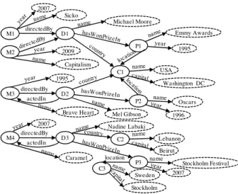
The most widely adopted data model specification for representing structured data in the web is RDF (Resource Description Framework). RDF syntax is based on XML and reflexes simple graph-based data model [1]. RDF represents data as triples < , , >. For instance, the fact that the movie Sicko (2007) is directed by Michael Moore from the USA can be represented by the following triples which form a directed labeled graph (see Figure 1):
< M1, name, Sicko > < M1, year, 2007 > < M1, directedBy, D1 > < D1, name, Michael Moore > < D1, country, C1 >
< C1, name, USA >
This way of representing data (RDF) is more elementary than databases and XML models, which indeed enables data integration and interoperability between systems. However, querying RDF data graphs is a major problem that brought the attention of the research community [5, 10, 16]. In fact, querying such data, which is typically stored in one relational table denoted by < , , > is of high complexity because traversing a graph stored in relational model involves many self-joins of that table. More specifically, a query with () edges on such a table requires
( − 1) self joins of that table [12].
Published As:
Anton Deik, Bilal Faraj, Ala Hawash, Mustafa Jarrar: Towards Query Optimization for the Data Web - Two Disk-Based algorithms: Trace Equivalence and Bisimilarity. In proceedings of the International Conference on Intelligent Semantic Web – Applications and Services. Pages 131-137. ACM. ISBN 9781450304757. June 2010.
Figure 1. An RDF Data graph
Several solutions were proposed to solve the problem of querying RDF. Among these are solutions which propose new methods for storing RDF such as Oracle’s Semantic Technology [7], C-Store [20, 3], and RDF3X [18]. Other solutions such as Graph-Signature Indexing [13] and PIG [22] use a different methodology; they propose to summarize RDF data such that queries are executed on the summaries instead of the original data. The latter solutions have shown better results in terms of performance and are more promising than those which propose alternative methods for storing RDF.
Summarizing data graphs as proposed by Graph-Signature Indexing [13] and PIG [22] is done using two well known algorithms, namely, Trace Equivalence and Bisimilarity. So far, versions of these algorithms were used to summarize relatively small XML data graphs [9, 14, 15, 17]. For instance, indexing techniques for XML such as DataGuides [9], 1-index [17], A(k)-index [15], and F&B [4, 14] all use Trace Equivalence and Bisimilarity algorithms for summarizing XML data. Also, versions of Trace Equivalence and Bisimilarity found in literature are memory based, that is, the data graph is loaded into the memory and the algorithms are executed there. In other words, memory-based versions of Trace Equivalence and Bisimilarity found in literature are not scalable due to the limitations imposed by the memory so they cannot be used to summarize large data graphs.
The original contribution of this paper is twofold; (i) to propose scalable disk-based versions of Trace Equivalence and Bisimilarity which can be used to summarize large data graphs and (ii) to adapt both algorithms to the RDF data model. The remainder of this article is arranged as follows: related work on indexing techniques is presented in section 2, our disk-based version of Trace Equivalence is discussed in section 3, and Bisimilarity in section 4. In section 5, we present an evaluation of our proposed algorithms on two relatively large datasets using different memory sizes.
Figure 2. The summary of the RDF data graph in Figure 1
2.
RELATED WORK
Several techniques have been proposed in the literature for indexing semi-structured data, especially for XML. Among these approaches are the DataGuides, 1-index, A(k)-index, and F&B. In this section we will briefly investigate each these indexing techniques.
The authors of [9] proposed the DataGuide as a covering index to answer queries from this index directly without referring to the original graph. The Dataguide is established by extracting all possible paths from a data graph. This technique is analogous to the problem of obtaining a deterministic automaton from a nondeterministic finite automaton. However, this approach relies on the graph being rooted (as the case in XML) as opposed to our approach that has no such structural constraint on the data. Moreover, a node can appear in the extent of more than one index node, allowing the index graph to be exponential in the size of the data graph at the worst case [17, 14]. On the contrary, the size of the index graph in our approach can never be larger than the size of the data graph. Further, DataGuides are not adequate for complex queries having several regular expressions and variables [17]. In practice, this approach becomes very problematic when applied to cyclic graphs, as the authors of [9] were unable to compute the strong DataGuide on a small subset of the IMDB dataset.
1-indicies proposed by [17] is another example of a covering index that covers incoming path queries. In this approach nodes having the same set of incoming paths are grouped together to obtain the index graph in a way similar to our approach. However, it also relies on the data graphs being rooted. Compared to DataGuides, the size of the 1-indicies has an upper bound dependent on the length of the longest acyclic path. Further, because grouping is based on the Bisimulation relationship, we can compute the index for a data graph with n nodes and m edges in (()) time, using an algorithm proposed by [19]. For highly irregular and heterogeneous data graphs, the size of the 1-index may become very large [17]. To tackle this issue the authors of [17] also proposed the T-index as a variant of the 1-indicies for reducing the size of the index. This is done by restricting the class of queries that the index supports. The A(k)-index proposed by [15] also reduces the size of the index by relaxing the equivalence condition, based on the concept of k-bisimilarity in which only paths whose length are no longer than k are considered.
Last of all, the F&B index proposed by [4, 14] group nodes having the same set of incoming (Forward) and outgoing (Backward) paths together. However, the size of this index can
M1,M2 M3,M4 2007, 2009 Capitalism, Sicko D1 actedIn D2, D3 1995, 2007 Brave Heart, Caramel P1,P2,P3 Michael Moore hasWonPrizeIn C1,C2,C3 Mel Gibson, Nadine Labaki USA, Lebanon, Sweden Washington DC, Stockholm, Beirut Emmy Awards, Oscars,
Stockholm Festival 1995,1996,2007 M1 M2 M3 2007 directedBy D1 Michael Moore P1 Emmy Awards 2009 C1 USA Washington DC directedBy D2 actedIn 1995 Brave Heart P2 Oscars 1996 M4 directedBy D3 actedIn 2007 Caramel Mel Gibson C2 Lebanon Beirut Nadine Labaki P3 Stockholm Festival 2007 name C3 Sweden Stockholm location 1995 Capitalism Sicko
approach the size of the data graph itself, giving a little performance gain when evaluating queries on the index instead of the original graph.
Our work in this paper differs from the related work briefed above in two issues. Firstly, our focus is on the RDF data model in that we adapt both Trace Equivalence and Bisimilarity algorithms to the RDF model. Secondly, all of these indexing techniques for XML data rely on memory-based versions of Trace Equivalence and Bisimilarity which are not scalable and thus cannot be used to summarize large datasets. On the contrary, our disk-based versions of Trace Equivalence and Bisimilarity are memory-independent and thus are scalable to very large data graphs.
3.
TRACE EQUIVALENCE
A data graph can be summarized by combining nodes that have exactly the same set of their outgoing paths. The graph shown in Figure 1 is summarized by the graph shown in Figure 2. For instance, one can notice that M1 and M2 have the same set of paths: {(name),
(year),
(directedBy, name),
(directedBy, country, name), (directedBy, country, capital), (directedBy, hasWonPrizeIn, name), (directedBy, hasWonPrizeIn, year),
(directedBy, hasWonPrizeIn, location, capital), (directedBy, hasWonPrizeIn, location, name)} Therefore, M1 and M2 are grouped together in the same category as shown in Figure 2. Also, M3 and M4 have the same set of their outgoing paths and therefore they are grouped together. However, they are not put into the same category as M1 and M2 because they don’t have the same set of paths; both M3 and M4 have an extra path: (directedBy, actedIn).
Generating such summaries is done using the well-known Trace Equivalence algorithm which we applied on the graph in Figure 1. Before delving into the definition of Trace Equivalence and the details of the algorithm, it is necessary to formally define the directed labeled graph and the vertex-rooted path which lies in the core of Trace Equivalence.
A directed labeled graph (also referred to here by data graph) is composed of vertices (nodes) and edges connecting those vertices. Labels are associated with all of the nodes and edges. The formal definition as proposed by [6] is as follows:
Definition 1. Given a finite set of vertex labels and a finite set
of edge labels , a directed labeled graph is defined by a triple
=< , , >, such that:
• is a finite set of vertices.
• ⊆ × is the relation that associates vertices with
labels, i.e., is the set of couples (, ) such that vertex
has label .
• ⊆ × × is the relation that associates edges with
labels, i.e., is the set of triples (, , ) such that edge
(, ) has label . From the definition of , we can define
the set of edges as: = (, ) | ∃, (, , )}.
Definition (2) below defines the vertex-rooted path and is based on Definition (1) of the directed labeled graph.
Definition 2.A v1-rooted path is defined as a finite tuple of edges
< (, ), (, ), … , (, ) >, such that, (, ) and
, are the same vertex ( = 1,2, … , ).
For simplicity, we can write the v1-rooted path as a finite tuple of edge labels< , , … , >, such that(, , )
( = 1,2, … , ).
Roughly speaking, Trace Equivalence is an equivalence relation defined on the set of vertices V, such that two vertices (, ) are Trace Equivalent if and only if the set of all -rooted paths is equal to the set of all -rooted paths. The more formal definition according to [11] is as follows:
Definition 3. The vertex trace-dominates the vertex if for every finite -rooted path , there is a -rooted path such that
= . The vertices and are trace equivalent, written ≈ if trace-dominates and trace-dominates .
Memory-based Trace Equivalence algorithm can be inferred from Definition (3) of Trace Equivalence relation. In literature, this definition is often presented as Trace Equivalence algorithm for graph summarization because the algorithm is indeed directly related to the definition. The algorithm simply suggests that we take each node in the graph and find all outgoing paths from it. After that, nodes having the same set of paths are grouped together. Each group is seen as an equivalent class of its members.
The memory-based version of the algorithm has been used to summarize directed labeled graphs, but proved to be inefficient if applied to large data graphs because of memory limitations. Hence, we introduce a scalable disk-based version of the algorithm to reduce large graphs. The idea in our version of the algorithm is basically based on the definition of Trace Equivalence relation (Definition 3); that is, to generate the summary of a graph we first find all possible outgoing paths of a node and then group the nodes that have the same set of paths together. However, in our disk based version of the algorithm a directed labeled graph is represented by a
< , , > table. So, finding the set of all paths from a node is done by continuously performing self-left joins to this table until all paths are determined. The number of self-left joins required depends on the levels the longest path spans, e.g., if the longest path is only two levels only one left join is needed, if it is four levels deep (as in our graph in Figure 1) then two left joins are needed, and so on. The stopping condition of this process is: “when no more left joins possible”, i.e., the longest path has been retrieved and further joins do not retrieve any additional path. However, because a self-left join becomes more expensive as the table becomes larger, the algorithm eliminates the columns that are not needed before performing each join. More specifically, the result of the first self-left join of the table < , , > is the table named
< , , , , , > (self-left join is done on = ).
Before performing the second self-left join we eliminate the columns < , > resulting in a reduced table, namely,
< , , , > on which the second self-left join is performed
resulting in the table < , , , , , , , >. Again,
before performing the third self-left join, columns < , >
are eliminated from this table resulting in the table <
, , , , , > on which the fourth self-left join is
performed. This elimination is done in the same manner for all remaining self-left joins. In addition, the algorithm checks for possible loops in the graph before performing the self-left join
because the existence of a loop would cause the algorithm to run indefinitely. The detection of the loop is done by checking the condition “ = ” for each row before performing the join and isolating the rows that satisfy this condition by copying them into a different table. After performing all required self-left joins and retrieving all paths, these rows are returned to the table.
However, it is worth mentioning that using Trace Equivalence is expensive; the process of testing the trace equivalence of two vertices in a directed labeled graph is known to be PSPACE complete [11]. It is not in the scope of this paper to improve the complexity of this process.
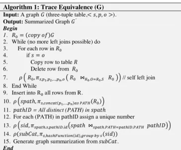
The algorithm is presented formally in Figure 3 using Relational Algebra notation.
Algorithm 1: Trace Equivalence (G)
Input: A graph (three-tuple table,< , , >).
Output: Summarized Graph ′
Begin
1. = ( )
2. While (no more left joins possible) do 3. For each row in
4. if =
5. Copy row to table
6. Delete row from
7. , ,,,…,, ⋈.. // self left join 8. End While
9. Insert into R all rows from R. 10. ℎ, ,(,…,) () 11. ℎ = All distinct (PATH) in ℎ
12. For each (PATH) in pathID assign a unique number
13. , .,.ℎ ⋈.. ℎ 14. (, ,(), ())
15. Generate graph summarization from .
End
Figure 3. The disk-based Trace Equivalence algorithm
4.
BISIMILARITY
The idea of using Bisimilarity for graph summarization was proposed as an improvement to tackle the complexity of the Trace Equivalence Algorithm. Bisimilarity algorithm produces summaries that are Trace Equivalent. However, these summaries are in fact approximations. In other words, the complexity of Bisimilarity algorithm is ( log ) for a graph with vertices and edges [11, 17] which is indeed a significant improvement on Trace Equivalence. However, Bisimilarity does not catch/summarize all cases, that is, some cases that are Trace Equivalent are skipped and not discovered by Bisimilarity. Again, as in section 2, we first present the well-known memory based algorithm for computing Bisimilarity (shown in Figure 4) and the definition of the Bisimilarity relation (given in Definition 4), then, we introduce our disk-based version of the algorithm.
Roughly speaking, Bisimulation in directed labeled graphs is an equivalence relation defined on a set of vertices , such that two vertices (, ) are Bisimilar if and only if the set of edge-labels of is equal to the set of edge-labels of . Also all nodes ’, ’ in the set of triples (, ’, ), (, ’, )} must be Bisimilar. This equivalence relation is written as ≈. Compared to Trace Equivalence, Bisimilarity relation is finer than Trace
Equivalence, that is ≈ implies ≈ [8, 11]. The formal
definition is given in Definition (4) below.
Definition 4. Given a directed labeled graph G=<V,rV,rE> as in Definition (1), two vertices (, ) ∈ are bisimilar if and only if: 1. For all set of tuples
< (,
, ), (, , ), … , (, , ) >∈ there
exists < (, , ), (, , ), … , (, , ) >∈
such that = ( = 1,2, … , ).
2. Conversely, for all set of tuples
< (,
, ), (, , ), … , (, , ) >∈ there
exists < (, , ), (, , ), … , (, , ) >∈ such
that = ( = 1,2, … , ).
3. The set of vertices (, ) ( = 1,2, … , ) are also
bisimilar.
procedure compute_bisim(G)
begin
1. Q and X are each a list of node-sets 2. Q = partition by label
3. X = (a copy of) Q 4. while (true) do
5. for each x in X do //stabilize Q w.r.t X 6. compute Succ(x)
7. for each q in Q do // split
8. replace q by q ∩ Succ(x) and q − Succ(x) 9. if there was no split then
10. break
11. X = (a copy of) Q
End
Figure 4. The memory-based Bisimilarity algorithm The Bisimilarity algorithm was used in the literature to summarize data graphs. In particular, several researchers used it to summarize XML graphs using several different techniques, such as 1-index [17], a(k)-index [15], and F&B [4,14].
However, RDF is more complex than XML in several ways. First of all, RDF data in its nature forms a graph, which means there is no single root for the data, whereas XML is tree structured, such that for every XML document there is only one single root for the data. Moreover, this tree structure implies the fact that every node in the graph has only one parent, and that for every node there is only one unique path that this node can be reached from. Conversely, in RDF the same node may be accessed via several paths, and through different nodes. Second, RDF may contain loops or cycles that should be taken in consideration when computing the structural summaries, compared to XML in which the summarization process is straightforward. These differences between XML and RDF impose the need to adapt the bisimilarity algorithm to become consistent with graph-based data. We will now demonstrate the basic ideas in the memory-based bisimilarity algorithm, and then we will discuss our disk-based version of the algorithm and its adaptation for large RDF graphs.
Compared to the Trace Equivalence algorithm, the Bisimilarity algorithm shown in Figure 4 creates graph summaries in an iterative process, such that in each iteration we group nodes up to a certain number of levels. Basically, the Bisimilarity algorithm produces a summarized graph in two steps. First, it groups the nodes based on the edge labels (or predicates in case of RDF). Second, these groups go through a number of iterations to split the nodes that conflict with the Bisimulation Equivalence relation, until no more splitting can be done. In
other word, after grouping the nodes with the same set of edge labels into categories, each group is taken alone and the successors of the nodes in the group are tested for Bisimilarity (this is done by checking the category of the successor node). Nodes whose successors fail the test are split from the group. For example, when applying Bisimilarity algorithm on the graph in Figure 1, one can notice that {M1, M2, M3, M4} have the same edge labels, {year, name, directedBy}. Hence, initially, these nodes are grouped in the same category. However, when their successors are tested for Bisimilarity, the algorithm reveals that the successor of M1, and M2 {D1} does not fall in the same category as the successor of M3 {D2} and M4 {D3}, thus we split the group {M1, M2, M3, M4} into {M1, M2} and {M3, M4}. This process typically goes over and over again until no more splitting is possible, that is, until the graph is stable. Figure 2 sketches the summarized graph in which one can notice how M1 and M2 are mapped to the same group, while M3 and M4 are mapped to another group. It is worth mentioning, that in our simple example, both Bisimilarity and Trace Equivalence algorithms resulted in the same summary. However, this is not always the case as clarified earlier.
In our disk-based version of the Bisimilarity algorithm, shown in Figure 5, our main focus was to propose an algorithm that is (i) disk based, and (ii) adapted to work on graph-based data such as RDF.
Algorithm 2: Bisimilarity (G)
Input: A Graph (three-tuple table, <S,P,O>)
Output: summarized Graph ´.
Begin
1. T0 = (Copy of) 2. T1 = all distinct (P) in T0
3. For each (P) in T1 assign a unique number
4. Update (P) in T0 with the corresponding unique number in T1 5. 1, ,(), ()
6. WHILE (R1 not stable)
7. , .,.,..⋈. . ⋈. . 8. 2, ,(), () ∩ , ()() 9. R1 = (copy of) R2 10. END WHILE
11. Generate graph summarization from R1
END
Figure 5. The disk-based Bisimilarity algorithm. In the memory-based version of Bisimilarity algorithm traversing all nodes to create groups of equivalent classes is expensive. Besides, testing successor nodes for Bisimilarity in a group of nodes has the complexity of (), whereas our disk-based version of the algorithm suggests a new way to create equivalent classes of Bisimilar nodes that has a complexity of ().
The initial grouping of nodes with similar outgoing predicates was done by assigning to each distinct predicate (P) a unique hash value. Then, we group all the nodes by the subject (S) and the sum of all its predicates hash value. Therefore, subjects that end up having the same summation belong to the same group. For example in Figure 1, let’s suppose that the outcome of the hash function for predicates {Country, name, hasWonPrizeIn, actedIn} was {1, 2, 3, 4} respectively. Computing the sum of predicates for {D1, D2, D3} yields {6, 10, 10} respectively. This means that D1 have a different set of predicates as opposed
to each of D2, and D3 which have the same set of predicates and therefore they are grouped together. Likewise, determining whether the successors of two nodes fall in the same category is done using the same idea. For all the subjects in the graph, we find their successors, and then we compute the sum of the subject category and a hash value of the sum of all its successors’ category together. Then, we group them by the subject. In this way, subjects in each group are split according to their successors’ categories. In general, this step is repeated times, until the table stabilizes, with corresponding to the longest acyclic path in the graph.
As mentioned earlier, because of the fact that the summaries created by the Bisimilarity algorithm are approximations, the size of the summary created is usually larger than the summary produced by the Trace Equivalence algorithm. This issue was not discussed in XML summarization techniques because for tree data graphs, the two equivalence relations (Bisimulation and Trace Equivalence) coincide [17]. However, this problem may easily appear in RDF because it forms a graph.
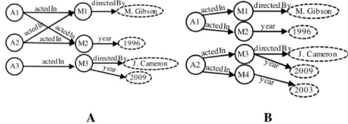
Our version of the Bisimilarity algorithm solves many of the problems that emerge in graph-based data (RDF), which does not appear in tree-structured data (XML). A typical problem is depicted in Figure 6.a, which emerges from the property that the edge labels coming out of a node are not unique. Using Trace Equivalence, nodes A1, A2, and A3 have the same set of paths, so they are grouped together. However, it’s not the case in the Bisimilarity algorithm, because the successors of these nodes do not fall in the same category. In our proposed version of the Bisimilarity algorithm, the hash function was carefully used to encrypt information about the predicates of the node which adapts the algorithm to solve this problem.
Another problem that appears in graph-based data which is discussed by [17], is depicted in Figure 6.b. One can notice that A1 and A2 are grouped together using the Trace Equivalence algorithm because they have the same set of paths. Meanwhile, these two nodes are not Bisimilar; because their successors (M1 and M3) do not belong to the same group. This case is what makes Bisimilarity algorithm produce larger summaries than Trace Equivalence algorithm.
However, as can be seen from our experiments in section 5, the difference in size between the summaries of the two algorithms can be tolerated; experimentally, the summary produced using the Bisimilarity algorithm is about 8% larger than that produced using Trace Equivalence. It is important to point out here that people using these summaries in query evaluation have to be aware not to use Bisimilarity algorithm to generate graph indexes when their query evaluation is based on Trace Equivalence scheme.
A B
Figure 6: Special cases that appear only in graph-based data A2 M1 M2 A1 M. Gibson 1996 actedIn actedIn directedBy year A3 M3directedBy J. Cameron 2009 actedIn year A1 M1 M2 directedBy M. Gibson 1996 A2 M3 M4 directedBy J. Cameron 2003 2009
5.
EXPERIMENTS EVALUATION
This section presents experimental results evaluating our disk- based versions of Trace Equivalence and Bisimilarity algorithms. Both algorithms were implemented using PL/SQL in Oracle 11g. The experiments were conducted on a PC with a 2.50 GHz Intel Core 2 Quad CPU, 2GiB of memory, and a 250GiB SATA Hard disk. The Operating System is Windows XP SP2.
In the experiments, we used two RDF datasets: the DBLP and Yago dataset. Yago contains 15 million triples (1.10GiB) while DBLP contains 8 million RDF triples (1.07GiB). We partitioned Yago into 5 tables: Y3 with 3 million triples, Y6 with 6 million, Y9 9 million, Y12 12 million, and Y15 with 15 million triples. DBLP was partitioned into 4 tables: D2, D4, D6, and D8 with 2, 4, 6, and 8 million triples respectively. Note that no sorting was applied on the data before partitioning (e.g., D4 was created by: create table D4 as select * from D8 where rownum<=4000000).
The two datasets we used in our experiments differ in the nature of the data they contain. The DBLP data tends to be more homogenous and node paths tend to be shorter than those in the Yago dataset (the longest path in the DBLP dataset is 4 levels long). On the contrary, Yago data is more heterogeneous and node paths tend to be longer than those in DBLP. These observations have an impact on the results of the experiments (shown in Tables 1 and 2) especially in the summarization time. For instance, in the case of Bisimilarity, Y6 is summarized in 241 seconds while D6 is summarized in 68 seconds though both contain 6 million triples. Also, to prove that our algorithms are indeed disk based and therefore memory independent, we conducted the same experiment twice on the same machine; the first was done using 2GiB of memory and the second was done using only 1GiB. Experimental results are summarized in Tables 1 and 2.
5.1
Analysis of Experimental Results
This subsection provides analysis of the experimental results shown in Tables 1 and 2 in terms of memory independency and scalability of both algorithms.
5.1.1
Memory independency of both algorithms
The results of our experiments prove that the two proposed algorithms are indeed disk based and thus memory independent. From Tables 1 and 2, one can see that reducing the memory used from 2GB to 1GB has no impact on the time cost of summarization for both algorithms.
5.1.2
Scalability evaluation
It is evident from the experimental results in either table that the time cost to summarize the graphs is linear with respect to the data size in both algorithms. For example, Bisimilarity-based summarization of D2 using 2GB of memory is 23 seconds, of D4 41 seconds, and of D6 68 seconds.
What is more scalable is the behavior of the graph summary with respect to the number of triples in the original graph. For instance, in the case of Trace Equivalence, the whole Yago dataset (Y15) is summarized by 462K triples. One can notice that this number tends to increase when the data is smaller (e.g. 658K for Y12). This means that it is likely that the more triples there are in the dataset, the more similarities are found, thus, the smaller the summary.
Table 1. Summary of Experimental results using our disk-based versions of Trace Equivalence and Bisimilarity algorithms on YAGO dataset
Number of Y3 Y6 Y9 Y12 Y15
Or ig in al G ra ph Unique Triples 3M 6M 9M 12M 15M Unique Subjects 1.78M 2.67M 3.30M 3.84M 4.34M Unique Predicates 81 83 83 84 84 Unique Objects 1.50M 3.04M 4.54M 6.09M 7.64M Data Size 226MiB 459MiB 678MiB 904MiB 1.10GiB
Gr ap h S u m m ar y (T ra ce E qu iv al en ce ) Unique Categories 32K 82K 121K 148K 100K
Triples in Summarized Graph 102K 312K 501K 658K 462K 2GiB Summarization Time
(seconds) 95 311 1,025 3,507 9,869 1GiB Summarization Time
(seconds) 94 314 1,022 3,511 9,873 Gr ap h S u m m ar y (B is im il ar it y ) Unique Categories 33K 86K 128K 159K 109K Triples in Summarized Graph 106K 325K 530K 703K 499K 2GiB Summarization Time (seconds) 96 241 504 1481 1,818 1GiB Summarization Time
(seconds) 101 243 498 1483 1,816
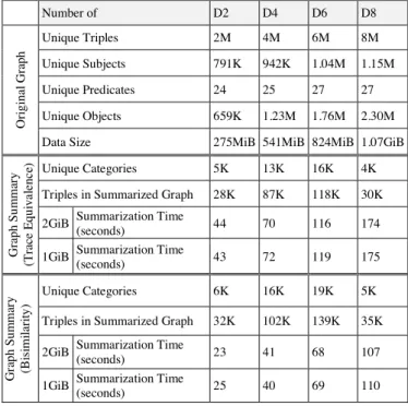
Table 2. Summary of Experimental results using our disk-based versions of Trace Equivalence and Bisimilarity algorithms on DBLP dataset
Number of D2 D4 D6 D8 Or ig in al Gr ap h Unique Triples 2M 4M 6M 8M Unique Subjects 791K 942K 1.04M 1.15M Unique Predicates 24 25 27 27 Unique Objects 659K 1.23M 1.76M 2.30M Data Size 275MiB 541MiB 824MiB 1.07GiB
Gr ap h S u m m ar y (T ra ce E q u iv al en ce ) Unique Categories 5K 13K 16K 4K
Triples in Summarized Graph 28K 87K 118K 30K 2GiB Summarization Time
(seconds) 44 70 116 174
1GiB Summarization Time
(seconds) 43 72 119 175 Gr ap h S u m m ar y (B is imi la ri ty ) Unique Categories 6K 16K 19K 5K Triples in Summarized Graph 32K 102K 139K 35K 2GiB Summarization Time
(seconds) 23 41 68 107
1GiB Summarization Time
6.
CONCLUSION AND FUTURE WORK
In this paper, we proposed two disk-based versions of the well-known Trace Equivalence and Bisimilarity algorithms for summarizing data graphs. Also, we adapted the algorithms to the RDF data model. The analysis of conducted experiments on both algorithms using relatively large RDF datasets proved that the two algorithms are scalable and totally memory independent. The research presented in this paper is part of the MashQL [13] project which aims to develop effective methods and techniques for querying the Data Web. This project was started at the University of Cyprus and is continued at Birzeit University. Future direction of this project is to develop a generalized query optimization solution for RDF data graphs, namely Graph-Signature Indexing which we plan to use for query optimization in MashQL.7.
ACKNOWLEDGEMENTS
First of all, we would like to express our gratitude and thanks for Mr. Majed Ayyad for his useful comments on earlier drafts of this paper.
We would also like to thank Professor Marios Dikaiakos and Mr. Andeas Manoli from the University of Cyprus for their generous help and contribution in the MashQL project. Without their help this research project wouldn’t have been possible.
8.
REFERENCES
[1] World Wide Web Consortium (W3C). http://www.w3c.org. (2010). [2] Linking Open Data Project.
http://esw.w3.org/topic/SweoIG/TaskForces/CommunityProj ects/LinkingOpenData (2009).
[3] Abadi, D.J., Marcus, A., Madden, S., and Hollenbach, K.J.”Scalable Semantic Web Data Management Using Vertical Partitioning”, In Proceedings of VLDB. 2007. [4] Abiteboul, S., Buneman, P., and Suciu, D. Data on the web:
from relations to semistructured data and XML. Morgan Kaufmann Publishers, Los Altos, CA 94022, USA, 1999. [5] Angles, R., and Gutierrez, C. Querying RDF data from a
graph database perspective, Proceedings of the 2nd European Semantic Web Conference (ESWC), Greece (2005), 346-360.
[6] Champin, P., and Solnon, C. Measuring the similarity of labeled graphs. In Proceedings of the Fifth International Conference on Case-Based Reasoning. Berlin. Springer, pp. 80–95. 2003.
[7] Chong, E., Das, S., Eadon, G., Srinivasan, J. An efficient SQL-based RDF querying scheme. VLDB ’05, Springer. 2005.
[8] Fernandez, J.C. An Implementation of an Efficient Algorithm for Bisimulation Equivalence. Science of Computer Programming, vol. 13, 2-3, may 1990.
[9] Goldman, R., and Widom, J. Dataguides: Enabling query formulation and optimization in semistructured databases, in VLDB, pages 436–445, 1997.
[10]Gutierrez, C., Hurtado, C., and Mendelzon, A. Formal aspects of querying RDF databases,First VLDB Workshop on Semantic Web and Databases,Berlin, Germany, September 7-8, 2003.
[11]Henzinger, R., Henzinger, A., and Kopke, W. Computing Simulations on Finite and Infinite Graphs. FOCS'95. [12]Jarrar, M., and Dikaiakos, M. A query formulation language
for the data web. IEEE Internet Computing Magazine. [13]Jarrar, M., and Dikaiakos, M. Querying the Data Web – The
MashQL approach. IEEE Internet Computing Magazine. 2010.
[14]Kaushik R, Bohannon P, Naughton J, Korth H: Covering Indexes for Branching Path Queries. SIGMOD’02 [15]Kaushik, R., Shenoy, P., Bohannon, P., and Gudes, E.
Exploting local similarity for efficient indexing of paths in graph structured data. ICDE, pages 129–140, 2002. [16]McGlothlin, J., and Khan, L. RDFJoin: A Scalable Data
Model for Persistence and Efficient Querying of RDF Datasets, Technical Report UTDCS-08-09.
[17]Milo, T., and Suciu, D. Index structures for path expressions. ICDT’99. 1999.
[18]Neumann, T., and Weikum, G. RDF3X: RISC style engine for RDF. VLDB’08.
[19]Paige, R., and Tarjan, R. E. Three partition refinement algorithms. SIAM Journal on Computing. 16(6):973{989, December 1987.
[20]Stonebraker, M., Abadi, D. J., Batkin, A., Chen, X., Cherniack, M., Ferreira, M., Lau, E., Lin, A., Madden, S., O’Neil, E. J., O’Neil, P. E., Rasin, A., Tran, N., and Zdonik, S. B. C-Store: A column-oriented DBMS. In VLDB, pages 553–564, 2005.
[21]Tian, Y., Hankins, R. A., and Patel, J. M. Efficient aggregation for graph summarization. Proceedings of the 2008 ACM SIGMOD international conference on Management of data, June 09-12, 2008.
[22]Tran, T. Efficient RDF Query Processing through Structure-aware RDF Graph Matching and Structure-based
Partitioning. A Technical Report
https://sites.google.com/site/kimducthanh/research/strucIdx-TR.pdf?attredirects=0&d=1