Socioeconomic Institute
Sozialökonomisches Institut
Working Paper No. 0404
Empirical Likelihood in Count Data Models:
The Case of Endogenous Regressors
Stefan Boes
Socioeconomic Institute University of Zurich
Working Paper No. 0404
Empirical Likelihood in Count Data Models:
The Case of Endogenous Regressors
March 2004
Author’s addresses Stefan Boes
E-mail: [email protected].
Publisher Sozialökonomisches Institut
Bibliothek (Working Paper) Rämistrasse 71 CH-8006 Zürich Phone: +41-1-634 21 37 Fax: +41-1-634 49 82 URL: www.soi.unizh.ch E-mail: [email protected]
Empirical Likelihood in Count Data Models:
The Case of Endogenous Regressors
Stefan Boes
∗University of Zurich
February 2004
Abstract
Recent advances in the econometric modelling of count data have often been based on the generalized method of moments (GMM). However, the two-step GMM procedure may perform poorly in small samples, and several empirical likelihood-based estimators have been suggested alternatively. In this paper I discuss empirical likelihood (EL) estimation for count data models with endogenous regressors. I carefully distinguish between parametric and semi-parametric methods and analyze the properties of the EL estimator by means of a Monte Carlo experiment. I apply the proposed method to estimate the effect of women’s schooling on fertility.
Keywords: Nonparametric likelihood, Poisson model, endogeneity, fertility and education.
JEL-Classification: C14, C25, J13
∗
Address for correspondence:University of Zurich, Socioeconomic Institute, Zuerichbergstr. 14, 8032 Zurich, Phone: +41 1 634 2301, E-Mail: [email protected]. I would like to thank Rainer Winkelmann, William Sander, and seminar participants at the University of Zurich for helpful comments.
1
Introduction
Count data models arise in many economic fields including health economics, demographic studies, labor economics, or industrial organization. Models for count data incorporate the special feature of the dependent variable being a nonnegative integer, or count. Examples are the number of doctor visits (Pohlmeierand Ulrich, 1995), the number of children born to women (Winkelmann and Zimmermann, 1995), the number of days a worker is absent from his job (DelgadoandKniesner,
1997), or the number of patents (Hausman, Hall andGriliches, 1984).
A serious problem occurring frequently in microeconomic applications is that of endogenous ex-planatory variables. This can be due to omitted variables, errors-in-variables, or more generally due to simultaneity, leading to inconsistency of parameter estimates obtained by standard methods. Within count data models endogeneity can be captured by additive or multiplicative errors in the mean function. Grogger (1990), Mullahy (1997), and Windmeijer and Santos Silva (1997)
discussed nonlinear instrumental variables, or generalized method of moments (GMM) to estimate regression parameters consistently.
Recent work concerning the properties of GMM in small samples or with increasing degree of over-identification emphasizes the poor performance of the two step GMM procedure. Several alter-native estimators were proposed, for example the continuous updating estimator (CUE) ofHansen,
Heaton and Yaron (1996), the empirical likelihood (EL) estimator of Owen (1988), Qin and
Lawless(1994) and Imbens(1997), and the exponential tilting (ET) estimator of Kitamura and
Stutzer(1997) andImbens, SpadyandJohnson(1998). All of these estimators can be subsumed
in the class of generalized empirical likelihood (GEL) estimators (Smith, 1997) and asymptotic equality of GEL and GMM was shown. Further studies of Newey and Smith (2000, 2004) and
Imbensand Spady(2001) examined the higher order properties of GEL and GMM estimators and
evidenced the relative advantage of EL compared to GMM and other GEL estimators in terms of smaller bias and higher order efficiency.
In this paper I discuss empirical likelihood estimation for count data models with endogenous regressors. I choose the empirical likelihood estimator due to its preferable properties and derive its first order conditions. I carefully distinguish between parametric and semi-parametric methods and analyze the properties of the estimator by means of a Monte Carlo experiment. As an empirical illustration of the proposed estimator I re-evaluate a study of Sander (1992) who analyzes the
effect of women’s schooling on fertility in the United States. Fertility is measured by the number of children ever born to a woman, thus the dependent variable is a count. Women’s schooling might be
endogenously determined because of non-zero correlation with unobservable traits. Sander (1992)
applies instrumental variables in a linear model, whereas Wooldridge (1997) tests in a Poisson
model. In addition to that I estimate the model with GMM and EL, and compare the different methods.
The outline of the paper is as follows. Preliminaries are laid out in Section 2. Section 3 considers empirical likelihood estimation. Section 4 compares EL with GMM and maximum likelihood. Section 5 gives results of a Monte Carlo study and Section 6 applies EL to estimate the effect of women’s schooling on fertility. Section 7 concludes.
2
Preliminaries
Econometric Modeling of Count Data
Letyi,i= 1, . . . , ndenote an independently distributed, nonnegative integer-valued variable with conditional mean specified as
E[yi|xi] =µi(β) = exp(xi0β), (1)
where xi is a k-dimensional vector of explanatory variables and β is a k-vector of unknown pa-rameters.1 A fully parametric assumption like the conditional distribution y
i|xi ∼ Poisson(µi(β)) allows for straightforward application of maximum likelihood methods. In the particular example of a Poisson process the maximum likelihood (ML) estimator of β, namely ˆβM L, solves the first order condition P
ixi(yi−µi(β)) = 0. From standard maximum likelihood theory it follows that ˆβM L is consistent and √n( ˆβM L−β) converges in distribution to a normal with mean zero and estimated variancen{P
iµi( ˆβM L)xixi0}−1, whereµi( ˆβM L) = exp(xi0βˆM L).
The standard Poisson model can be misspecified for several reasons. For example the assumption of equidispersion – the equality of mean and variance – is frequently violated in applied work and more general distributions are developed to cover features like over- or underdispersion.2 However,
Gourieroux, Monfort and Trognon(1984) showed that Poisson estimates are still consistent
as long as the conditional mean is properly specified. Correct standard errors can be obtained by the estimated variance of the pseudo maximum likelihood (PML) estimator ˆβP M L (= ˆβM L), which
1
For a discussion of count data models in respect of theory and practical applications seeWinkelmann(2003).
2
Examples are the negative binomial (negbin) and the logarithmic distribution, or mixture distributions, again see
can be calculated by ˆV( ˆβP M L) = n X i=1 µi( ˆβP M L)xixi0 !−1 n X i=1 yi−µi( ˆβP M L) 2 xixi0 ! n X i=1 µi( ˆβP M L)xixi0 !−1 , (2)
whereµi( ˆβP M L) = exp(xi0βˆP M L) = exp(xi0βˆM L).
Generalized Method of Moments
Since the seminal article ofHansen (1982) generalized method of moments (GMM) has become
a well-established estimation technique in applied and theoretical econometrics. GMM provides a general framework for dealing with moment conditions avoiding strong distributional assumptions. The specification of a conditional mean in (1) defines implicitly a conditional moment restriction E[ui|xi] = 0, where ui is a regression error with ui = yi−µi(β). The law of iterated expectations proves thatk unconditional moment restrictions can be constructed as
E[xi(yi−µi(β))] = 0. (3)
The GMM estimator ˆβGM M minimizes the weighted squared distance of sample and population moments, algebraically ˆ βGM M = arg min β 1 n n X i=1 xi(yi−µi(β)) !0 W 1 n n X i=1 xi(yi−µi(β)) ! , (4)
where W is weighting matrix. Since (3) is an exactly determined equation system, the GMM first order conditions are unaffected by the choice of W and identical to the ML first order conditions, hence ˆβGM M = ˆβM L. Under mild regularity conditions one can show the consistency and asymptotic normality of the GMM estimator.3 The efficient GMM estimator can be obtained for the appropriate
choice of weights which is W = V[P
ixi(yi −µi(β))]. If the weighting matrix W is estimated by n{P
i(yi−µi( ˆβGM M))2xixi0}−1, the variance of ˆβGM M is equal to that of ˆβP M L.
Endogenous Regressors
As mentioned above the consistency of ML and PML estimation crucially depends on the as-sumption of valid moment conditions, i.e. E[yi|xi] = µi(β) holds. In other words, a misspecified mean function leads to inconsistency of ˆβM L and ˆβP M L. The problem of endogeneity can be seen as one example in which the moment condition fails. Recent contributions on endogenous regressors
3
within count data models (Windmeijer and Santos Silva, 1997; Mullahy, 1997) consider two
alternative approaches: (1) endogeneity with additive errors and (2) endogeneity with multiplicative errors.
The case of additive errors leads to a conditional mean function of the form
E[yi|xi, ξi] = exp(xi0β) +ξi, (5)
where endogeneity is present if E[ξi|xi]6= 0 and I assume the existence of aq-dimensional vector of instrumentszi(q≥k) such thatE[ξi|zi] = 0. Again by the law of iterated expectations unconditional moment restrictions are
E[zi(yi−µi(β))] = 0, (6)
which can be estimated by GMM replacing the moment functionsxi(yi−µi(β)) in (4) by the functions zi(yi−µi(β)).4 A more intuitive approach to deal with endogenous regressors is to treat unobservable factorsεi and regressors xi symmetrically and to specify a mean function with multiplicative errors as
E[yi|xi, εi] = exp(xi0β+εi) =µi(β)νi, (7)
where νi = exp(εi). The conditional expectation with respect to xi is E[yi|xi] =µi(β)E[νi|xi] and endogeneity is present if E[νi|xi]6= 1. In this case I assume that instruments zi are available such that E[νi|zi] = 1 and conditional moment restrictions are given by E[νi −1|zi] = 0. The law of iterated expectations shows that
E zi yi−µi(β) µi(β)
= E[zi(exp(−xi0β)yi−1)] = E[zi(νi−1)] = 0. (8)
WindmeijerandSantos Silva(1997) emphasized that a set of instrumentszicannot be orthogonal toξi (the additive case) and νi−1 (the multiplicative case) at the same time sinceyi−µi(β) and µi(β) are correlated. In this paper I concentrate on endogeneity with multiplicative errors, although all results are easily extended to the additive case.
The moment conditions in (8) can be estimated by GMM as presented in the preceding paragraph. An interesting case arises when the number of instrumentsqexceeds the number of regressorsk(the over-determined case), and one can apply a two step GMM procedure to estimate the parametersβ in (8). The efficient estimator ˆβGM M2 is the argument β that minimizes the objective function
1 n n X i=1 zi yi−µi(β) µi(β) !0 ˜ V−1 1 n n X i=1 zi yi−µi(β) µi(β) ! , (9)
where ˜V−1 =n−1P
i{(yi−µi( ˜β))/µi( ˜β)}2zizi0 are the optimal weights withµi( ˜β) = exp(xi0β˜), and ˜
β is a first step GMM estimator using any weighting matrix W, e.g. the q-dimensional identity matrix. Under mild regularity conditions ˆβGM M2 is consistent and the stabilizing transformation √
n( ˆβGM M2−β) is asymptotically normal with mean zero and estimated variance
1 n n X i=1 ziyixi0 µi( ˆβGM M2) !0 1 n n X i=1 yi−µi( ˆβGM M2) µi( ˆβGM M2) !2 zizi0 −1 1 n n X i=1 ziyixi0 µi( ˆβGM M2) ! −1 , (10) whereµi( ˆβGM M2) = exp(xi0βˆGM M2).
3
Empirical Likelihood Estimation
Based upon the work ofOwen(1988, 1991, 2001) andQinandLawless(1994, 1995) I now develop
the empirical likelihood (EL) estimator of β for the conditional mean specification (1) taking into account thatximay be endogenous in a multiplicative sense, thus considering unconditional moment restrictions (8).
Letpi denote the unknown probability assigned to the sample outcome (yi, xi, zi) of one observa-tion iwith 0≤pi ≤1 ∀i and impose a normalization Pipi = 1. Furthermore, let p= (p1, . . . , pn)0 denote the n-dimensional vector of probabilities. Then a nonparametric likelihood estimator ofp is obtained from maximizing a nonparametric log-likelihood function,
max p n −1 n X i=1 lnpi s.t. n X i=1 pi= 1. (11)
Without further restrictions optimal probability weights in (11) are given bypi =n−1, the empirical density function. To incorporate special features of the data generating process impose empirical moments as additional restrictions. From (8), aq-dimensional vector of empirical moment conditions can be specified as n X i=1 pizi yi−µi(β) µi(β) = 0. (12)
Note the difference between sample moments, where each observation is weighted by n−1, and the
empirical moments in (12), where each observation is weighted bypi. The optimization problem in (11) using the additional restrictions in (12) can be rewritten as
max p n −1 n X i=1 lnpi s.t. n X i=1 pizi yi−µi(β) µi(β) = 0, n X i=1 pi= 1, (13)
which implies the optimality conditions pi(β) = 1 n h 1−λ(β)0zi yi−µi(β) µi(β) i and (14) λ(β) = argλ n X i=1 zi yi−µi(β) µi(β) n h 1−λ(β)0zi yi−µi(β) µi(β) i = 0 , (15)
whereλ(β) is aq-dimensional vector of Lagrangean multipliers with respect to the empirical moment restrictions. Plugging (14) and (15) into the objective function in (13) yields an empirical log-likelihood function, lnLEL(β) =−ln(n)−n−1 n X i=1 ln 1−λ(β)0zi yi−µi(β) µi(β) . (16)
The maximum of (16) is the value ofβ, namely the empirical likelihood estimator ˆβEL, that simul-taneously solves n X i=1 −xiyizi 0λ( ˆβ EL) µi( ˆβEL) n h 1−λ( ˆβEL) 0 zi yi−µi( ˆβEL) µi( ˆβEL) i = 0 (17) n X i=1 zi yi−µi( ˆβEL) µi( ˆβEL) nh1−λ( ˆβEL)0zi yi−µi( ˆβEL) µi( ˆβEL) i = 0, (18)
where (18) follows directly from the optimality condition (15). Since (17) and (18) build up a highly non-linear equation system, numerical methods have to be applied to obtain the value of ˆβEL.
Under similar regularity conditions as in the GMM frameworkQinand Lawless(1994) showed
the consistency of the empirical likelihood estimator and proved the asymptotic normality of the stabilizing transformation √n( ˆβEL−β) with mean zero and estimated variance
( n X i=1 pi( ˆβEL) ziyixi0 µi( ˆβEL) !0 × n X i=1 pi( ˆβEL) yi−µi( ˆβEL) µi( ˆβEL) !2 zizi0 −1 n X i=1 pi( ˆβEL) ziyixi0 µi( ˆβEL) ! )−1 , (19)
where pi( ˆβEL) is given by (14) evaluated at ˆβEL. Note that the terms in (19) are estimated by probability weights obtained from an empirical likelihood optimization whereas the terms in (10) are estimated by probability weightsn−1. One important feature of EL and efficient GMM is, relating to the work ofChamberlain(1987), that both estimators reach the semiparametric efficiency bound.
4
Interpretation of Empirical Likelihood Estimates
Comparing the First Order Conditions of GMM and EL
In the spirit of Newey and Smith (2004) and to get a deeper understanding of generalized
method of moments and empirical likelihood estimation in the count data framework, I compare the first order conditions of both estimators. The optimization in (9) gives the first order conditions of the two step GMM estimator, algebraically
n X i=1 1 n ziyixi0 µi( ˆβGM M2) !0 n X i=1 1 n yi−µi( ˜β) µi( ˜β) !2 zizi0 −1 1 n n X i=1 zi yi−µi( ˆβGM M2) µi( ˆβGM M2) !! = 0, (20)
where ˜β is the first round estimator. In the context of empirical likelihood estimation one can show that conditions (17) and (18) imply first order conditions5
n X i=1 pi( ˆβEL) ziyixi0 µi( ˆβEL) !0 × n X i=1 pi( ˆβEL) yi−µi( ˆβEL) µi( ˆβEL) !2 zizi0 −1 1 n n X i=1 zi yi−µi( ˆβEL) µi( ˆβEL) !! = 0. (21) Equations (20) and (21) show the main difference between GMM and EL. Each estimator sets a linear combination of sample moments equal to zero, where the sample moments are given by the right brackets in both equations. GMM and EL differ in the way of calculating these linear combinations. GMM uses sample moments for the Jacobian matrix (left brackets) and the matrix of second moments (middle brackets). Furthermore, the weighting matrix depends on a first step (inefficient) estimator. In contrast to that EL uses empirical moments for the Jacobian term and the matrix of second moments, whereby the probability weights pi are chosen efficiently.
Relationship to Maximum Likelihood Estimation
In a standard Poisson model the conditional probability functionf(yi|xi;β) is given by
f(yi|xi;β) =
exp(−exp(x0iβ)) exp(yix0iβ) yi!
, (22)
which follows directly from the conditional mean specification (1) and the distributional assumption yi|xi ∼Poisson(µi(β)). The (parametric) sample likelihood function can be written as L(β;y, x) = Qn
i=1f(yi|xi;β) and the maximum likelihood estimator chooses the value ofβsuch that the observed
sample is most likely. Once estimates of β are obtained, the parametric specification allows for a
5For a general derivation and interpretation see
discussion of marginal probability effects, i.e. the effect of a small ceteris paribus increase in one regressor on the probability of observing a certain outcome of y. Furthermore, one can calculate probabilities of outcomes that are not observed in the sample.
Within empirical likelihood estimation parameterspi of a joint probability mass function Qn
i=1pi are defined, and this function is maximized with respect to constraints defined in terms of empirical moment conditions. The probability mass function can be interpreted as a multinomial distribution with nparameters pi, one parameter for each data outcome (yi, xi, zi). Moreover, one can think of constrained maximum likelihood estimation ofpwith constraints represented by empirical moments and a natural normalization for probability functions, P
ipi = 1. As noted in the previous section probability weightsn−1 are optimal if empirical moments are absent or moment restrictions (8) dis-play an exactly determined equation system. The latter follows since optimal Lagrangean multipliers are zero in this case. If the number of instruments is larger than the number of parameters (the over-determined case),λ( ˆβEL) differs from zero andpi( ˆβEL) differs fromn−1. Information theoretic approaches show that pi( ˆβEL) is chosen as close as possible to n−1 taking into account that the empirical moments have to be fulfilled (see Kitamura and Stutzer (1997) and Imbens, Spady
and Johnson(1998)).
Two important conclusions can be drawn from the preceding discussion. First, we cannot compare probabilities pi with a parametrically specified conditional probability function like the Poisson, or any other count data distribution. A conditional probability functionf(yi|xi;β) gives the probability of observing one of the values yi = 0,1,2, . . . given a vector of explanatory variables xi, whereas pi gives the sample probability of one observation. Second, empirical likelihood estimates of pi do not allow for calculation of marginal probability effects or prediction of probabilities of outcomes that are not observed in the sample.
5
Monte Carlo Evidence
In this section I illustrate the theoretical advantage of empirical likelihood estimation by means of a Monte Carlo experiment. I choose different sample sizes (n = 100, 500, and 1000), and for each sample size 1000 vectors of y are drawn from a Poisson distribution with parameter µi = exp(0.5−x1i−0.5 ˜x2i+εi), hence the true parameter vector isβ0 = (0.5 −1 −0.5)0. The regressorsx1i and ˜x2i are independently and uniformly distributed on the interval [0,1], the unobservable factorsεi are independent drawings from a normal distribution with mean zero and variance 0.7. I assume that
˜
x2i cannot be observed butx2i = ˜x2i+vi, where vi is a classical measurement error independently and normally distributed with mean zero and variance equal to one. To complete the story I generate different instrumentszi with properties corr(zi, x2i) =ρ and corr(zi, εi) = 0 which allows us to vary the number and quality of instruments by choosing different values ofρ.
There is a large number of possible combinations of instruments and sample sizes and there-fore I picked out just a few. Precisely, for each sample size I define weakly identified setups (3 instruments withρ= 0.1,0.1,0.5), partial identified setups (3 instruments withρ= 0.5,0.5,0.5 or ρ = 0.1,0.5,0.9), and strong identified setups (3 instruments with ρ = 0.9,0.9,0.9). For n= 500 observations and partial identification I increase the number of instruments to five and ten (all in-struments with ρ = 0.5 or evenly distributed between 0.1 and 0.9). All setups are estimated by GMM and EL, and for the sake of completeness the PML estimator is calculated for all sample sizes. As mentioned above numerical methods have to be applied to obtain the EL estimator. I use the BFGS (Broyden, Fletcher, Goldfarb, Shanno) algorithm as it is implemented in theconstrained
optmum procedure of Gauss6 and maximize the empirical likelihood function in (16) with respect
toβ and λ, and subject to the constraint in (15). PML and GMM estimators are calculated by the same algorithm, maximizing the parametric likelihood function of a Poisson model and minimizing the GMM objective function in (4) respectively. The results are reported in Tables 1 to 4.
— Table 1 about here —
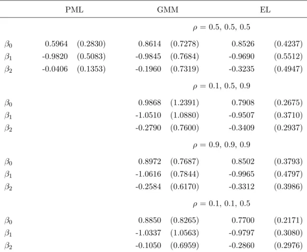
Table 1 gives the results for a sample size ofn= 100 observations. For each estimator I calculate the mean and standard deviation of the beta’s (standard deviation in parentheses). As we would expect, the PML estimate of β1 is unaffected by the measurement error, but the estimate of β2 is
biased and inconsistent. As in the linear model with classical errors-in-variables we have a regression to the mean, i.e. the parameter estimate is biased towards zero. GMM and EL estimates ofβ1 do
not differ considerably from PML estimates, but estimates ofβ2 are closer to the true value of−0.5.
Moreover, GMM and EL estimates are substantially different. The bias of EL is less than the bias of GMM, particularly in the case of weakly correlated instruments, and standard deviations are smaller.
— Tables 2 and 3 about here —
6
Tables 2 and 3 give the results for the same set of instruments but two different sample sizes, n= 500 andn= 1000. EL as well as GMM estimates ofβ2 get closer to the true value and standard
deviations of all estimates decrease. Only in the case of 500 observations and weak identification EL is notably closer to −0.5 than GMM. With 1000 observations differences between both estimators disappear independently of varying the quality of instruments. I emphasize that both estimators perform much better in the case of strong identification, or in other words the presence of weak instruments causes both estimators to be more biased. Another important result is that throughout different setups EL has smaller standard deviations than GMM.
— Table 4 about here —
Table 4 shows the results for partial identification with five or ten instruments and a sample size of 500 observations (only 500 replications are calculated). Five instruments with ρ= 0.5 cause the GMM estimator to be more biased compared to the case of three instruments, whereas the EL estimator performs approximately the same. With correlations between 0.1 and 0.9 discrepancies between EL and GMM disappear. Ten instruments withρ = 0.5 again cause the GMM estimate of β2 to be more biased than EL. Parameter estimates are similar to the case of five instruments, but
standard deviations are larger. Evenly distributed correlations between 0.1 and 0.9 show approxi-mately the same estimates as with five instruments, but standard deviations of the GMM estimator increase substantially. These results support theoretical findings of Newey and Smith (2004) and Imbens and Spady (2001) that with increasing number of instruments and decreasing number of
observations GMM may be more biased than EL.
So far, I have only considered the standard deviation of the beta’s and not the mean of the estimated standard errors based on the asymptotic distribution. Hence, I distinguish between robust point estimates and inference. In fact I calculated both values, and with a sample size of 1000 observations they are approximately the same. But with sample sizes of 100 or 500 observations the two values differ substantially, in particular in the case of weak identification. Therefore, the classical normal asymptotic approximations to the finite-sample distributions are very poor. This result is not surprising since recent work concerning the properties of GMM and EL estimators under weak identification shows nonstandard distributions (see e.g. Stock, Wright and Yogo, 2002,
andGuggenbergerandSmith, 2003). Inference can be improved by using bootstrapped standard
errors or by applying methods proposed in the above-quoted literature, such as tests based on the objective function (16).
6
An Empirical Example
As an illustration of empirical likelihood estimation in count data models with endogeneity, I consider a data set similar to that used bySander(1992) andWooldridge(1997) taken from the National
Opinion Research Center’s General Social Survey. I used the same independent and pooled cross-sections across even years from 1972 to 1984 as inWooldridge(1997) with the number of siblings
(sibs) as additional variable.7 The variables of interest are the number of children ever born to women
(childs) as dependent count variable, and years of schooling (schooling) as explanatory variable to determine the effect of women’s schooling on fertility. Additional controls are quadratic age (age, agesq), a dummy for race (black), region at age sixteen (relative to south), type of residence at age sixteen (relative to big cities), and time dummies for the even years from 1974 to 1984. As discussed inSander(1992) schooling might be endogenous in the fertility regression, e.g. due to unobservable
traits correlated with schooling.
In the sample of 992 women between the ages of 35 and 54 the average number of children is 2.7 (standard deviation 1.6) and on average a woman attends 12.9 (2.6) years of schooling. First of all assuming schooling is exogenous I estimate a linear model and a Poisson model with robust standard errors. The results are reported in Table 5, columns OLS and PML. The coefficient on schooling in the linear model is -0.11 with a t-statistic of -5.70, thus the estimate is highly significant. Economically, given one more year of schooling the expected reduction in the number of children is 0.11. In other words, attending a university for 5 years reduces the expected number of children about a half compared to a woman who does not attend a university. Note that interpretation in the linear model is somewhat misleading because negative predicted outcomes for the dependent count variable are possible. In the Poisson model the estimated coefficient on schooling is -0.0428 with a standard error of 0.0086 which implies that the coefficient is statistically significant and each additional year of schooling reduces the number of children about 4.3 percent. Multiplying the coefficient on schooling in the Poisson model by the average number of children shows that the implied marginal effect at the sample means is about the same as in the linear model.
— Table 5 about here —
7
Sander(1992) uses data from 1985 to 1991. The data set is available from the data archive ofWooldridge’s
(2003) textbook for even years 1972 to 1984 (withoutsibs). The whole data set collected for almost all years between 1972 and 1994 is freely available online at http://www.soc.qc.edu/QC Software/GSS.html. Comprehensive information on theGeneral Social Surveyincluding the data set for almost all years between 1972 and 2002 can be found online at http://www.norc.uchicago.edu/projects/gensoc.asp and http://www.icpsr.umich.edu:8090/GSS/homepage.htm.
For possibly endogenous schooling I use father’s and mother’s schooling, and the number of siblings as instruments. A simple OLS regression of schooling on the instruments controlling for the other variables shows highly significant instruments. Wooldridge(1997) tests for endogeneity by adding
the residuals from this regression to his original Poisson model and computing the corresponding t-statistic. Within a linear modelSander(1992) tests for endogeneity with a simple Hausman test. I replicate these tests and conclude thatschoolingis not highly endogenous in the fertility equation, a result similar to those ofSander (1992) and Wooldridge(1997).
Nevertheless, I apply instrumental variable estimation of the fertility equation using two stage least squares (2SLS), GMM, and EL. The results are reported also in Table 5. Estimating the linear model with 2SLS yields a highly significant coefficient on schooling of -0.1661 (0.0400). Thus the effect of schooling is more negative compared to OLS meaning that schooling and unobservable traits are positively correlated. The GMM estimate of the effect of schooling is -0.0669 (0.0168), the EL estimate is -0.0740 (0.0166). Both are significant on the one percent level, EL implying a 7.40 percent decrease in the number of children given one more year of schooling (GMM: 6.69 percent). Of particular interest in the context of instrumental variable estimation and over-determined restrictions is the validity of moments. In the GMM framework this can be tested based on the value of the objective function (9) evaluated at the GMM estimator (the J-Test). Within empirical likelihood estimation a test can be based on a likelihood ratio statistic, namely the scaled by 2ndifference of the log-likelihood function (16) evaluated at pi =n−1 andpi( ˆβEL) respectively. Both test statistics are asymptotically chi-squared distributed under the null hypothesis of valid moment equations, with a critical value of χ2(2),0.95= 5.99 at 5 percent level of significance. The values of the over-identifying test statistics are reported in Table 5 (GMM: 0.39, EL: 0.67), thus both tests cannot reject the null of valid moment restrictions.
7
Conclusions
In this paper I developed the empirical likelihood estimator for a count data model with standard mean specification taking into account that regressors might be endogenously determined. I consid-ered the case of multiplicative errors in the mean and derived the first order conditions for the EL estimator. Based on Monte Carlo simulations I showed that empirical likelihood can improve upon GMM, particularly in situations when samples are small and instruments are weak. In such cases the use of EL is therefore strongly recommended.
Empirical likelihood as applied here estimates a count data model without assuming a conditional distribution function, and only specifying the mean function. These weak assumptions allow for robust estimation of the parameters of interest and results of the Monte Carlo experiment support this argument. On the other hand, we forego the possibility of predicting (out of sample) probabilities and calculating marginal probability effects.
In an empirical application, the EL method was used to estimate the effect of women’s schooling on fertility based on 992 pooled cross sectional observations of the General Social Survey for even years from 1972 to 1984. To account for potential endogeneity of schooling, parent’s schooling and the number of siblings were used as instruments. The EL point estimate of the schooling effect was substantially below the standard Poisson estimate. However, the null hypothesis of no endogeneity could not be rejected.
References
Chamberlain, G.(1987): “Asymptotic Efficiency in Estimation with Conditional Moment
Restric-tions,” Journal of Econometrics, 34, 305–334.
Delgado, M., and T. Kniesner(1997): “Count Data Models with Variance of Unknown Form:
An Application to a Hedonic Model of Worker Absenteeism,”Review of Economics and Statistics, 79, 41–49.
Gourieroux, C., andA. Monfort(1995): Statistics and Econometric Models, vol. 1. Cambridge
University Press, Cambridge.
Gourieroux, C., A. Monfort, and A. Trognon (1984): “Pseudo Maximum Likelihood
Meth-ods: Applications to Poisson Models,” Econometrica, 52, 701–720.
Grogger, J. (1990): “A Simple Test for Exogeneity in Probit, Logit, and Poisson Regression
Models,”Economics Letters, 33, 329–332.
Guggenberger, P., and R. Smith (2003): “Generalized Empirical Likelihood Estimators and
Tests under Partial, Weak and Strong Identification,” cemmap working paper 08/03.
Hansen, L., J. Heaton, and A. Yaron (1996): “Finite-Sample Properties of Some Alternative
GMM Estimators,”Journal of Business & Economic Statistics, 14, 262–280.
Hansen, L. P.(1982): “Large Sample Properties of Generalized Method of Moments Estimators,”
Econometrica, 50, 1029–1054.
Hausman, J., B. Hall, and Z. Griliches(1984): “Econometric Models for Count Data with an
Application to the Patents - R&D Relationship,” Econometrica, 52, 909–938.
Imbens, G.(1997): “One-Step Estimators for Over-Identified Generalized Method of Moment
Mod-els,” Review of Economic Studies, 64, 359–383.
Imbens, G., andR. Spady (2001): “The Performance of Empirical Likelihood and its
Generaliza-tions,” paper presented at 2001 NSF-Berkeley Econometrics Symposium on ”Identification and Inference for Econometric Models.
Imbens, G., R. Spady, andP. Johnson(1998): “Information Theoretic Approaches to Inference
Kitamura, Y., and M. Stutzer (1997): “An Information-Theoretic Alternative to Generalized
Method of Moments Estimation,” Econometrica, 65, 861–874.
Mullahy, J. (1997): “Instrumental-Variable Estimation of Count Data Models: Applications to
Models of Cigarette Smoking Behavior,” Review of Economics and Statistics, 79, 586–593.
Newey, W., and R. Smith (2000): “Asymptotic Bias and Equivalence of GMM and GEL
Esti-mators,” unpublished working paper no. 01/517, University of Bristol.
(2004): “Higher Order Properties of GMM and Generalized Empirical Likelihood Estima-tors,” Econometrica, 72, 219–255.
Owen, A. (1988): “Empirical Likelihood Ratio Confidence Regions for a Single Functional,”
Biometrika, 75, 237–249.
(1991): “Empirical Likelihood for Linear Models,” Annals of Statistics, 19, 1725–1747. (2001): Empirical Likelihood. Chapman & Hall/CRC, Boca Raton.
Pohlmeier, W., andV. Ulrich(1995): “An Econometric Model of the Two-Part Decisionmaking
Process in the Demand for Health Care,” Journal of Human Resources, 30, 339–361.
Qin, J.,andJ. Lawless(1994): “Empirical Likelihood and General Estimating Equations,”Annals
of Statistics, 22, 300–325.
(1995): “Estimating Equations, Empirical Likelihood, and Constraints on Parameters,”
Canadian Journal of Statistics, 23, 145–159.
Sander, W.(1992): “The effect of women’s schooling on fertility,”Economics Letters, 40, 229–233. Smith, R.(1997): “Alternative Semi-Parametric Likelihood Approaches to Generalised Method of
Moments Estimation,” Economic Journal, 107, 503–519.
Stock, J., J. Wright, and M. Yogo (2002): “A Survey of Weak Instruments and Weak
Iden-tification in Generalized Method of Moments,” Journal of Business & Economic Statistics, 20, 518–529.
Windmeijer, F. A. G.,andJ. M. C. Santos Silva(1997): “Endogeneity in Count Data Models:
Winkelmann, R. (2003): Econometric Analysis of Count Data. Springer Verlag, Berlin.
Winkelmann, R., and K. Zimmermann (1994): “Count Data Models for Demographic Data,”
Mathematical Population Studies, 4, 205–221.
Wooldridge, J. (1997): “Quasi-Likelihood Methods for Count Data,” in Handbook of Applied
Table 1: Monte Carlo results part 1 (n= 100, 3 instruments forx2) PML GMM EL ρ = 0.5, 0.5, 0.5 β0 0.5964 (0.2830) 0.8614 (0.7278) 0.8526 (0.4237) β1 -0.9820 (0.5083) -0.9845 (0.7684) -0.9690 (0.5512) β2 -0.0406 (0.1353) -0.1960 (0.7319) -0.3235 (0.4947) ρ = 0.1, 0.5, 0.9 β0 0.9868 (1.2391) 0.7908 (0.2675) β1 -1.0510 (1.0880) -0.9507 (0.3710) β2 -0.2790 (0.7600) -0.3409 (0.2937) ρ = 0.9, 0.9, 0.9 β0 0.8972 (0.7687) 0.8502 (0.3793) β1 -1.0616 (0.7844) -0.9965 (0.4797) β2 -0.2584 (0.6170) -0.3312 (0.3986) ρ = 0.1, 0.1, 0.5 β0 0.8850 (0.8265) 0.7700 (0.2171) β1 -1.0337 (1.0563) -0.9797 (0.3080) β2 -0.1050 (0.6959) -0.2860 (0.2976)
first value: mean ofβ’s, second value (in parentheses): standard deviation ofβ’s; 1000 replications true model:E[yi|xi] = exp(0.5−x1i−0.5 ˜x2i+εi),εi∼N(0,0.7)
Table 2: Monte Carlo results part 2 (n= 500, 3 instruments forx2) PML GMM EL ρ = 0.5, 0.5, 0.5 β0 0.6235 (0.1260) 0.9405 (0.3473) 0.9198 (0.2095) β1 -1.0021 (0.2216) -1.0086 (0.2713) -0.9878 (0.2317) β2 -0.0403 (0.0628) -0.4389 (0.2826) -0.4438 (0.2106) ρ = 0.1, 0.5, 0.9 β0 0.9186 (0.4016) 0.8893 (0.2046) β1 -1.0285 (0.2713) -1.0064 (0.2260) β2 -0.3817 (0.3454) -0.3928 (0.2344) ρ = 0.9, 0.9, 0.9 β0 0.9500 (0.3413) 0.9077 (0.1863) β1 -0.9967 (0.3215) -0.9787 (0.2347) β2 -0.4561 (0.2884) -0.4409 (0.1837) ρ = 0.1, 0.1, 0.5 β0 0.8938 (0.4709) 0.8361 (0.2231) β1 -1.0004 (0.2915) -0.9616 (0.2650) β2 -0.3106 (0.4290) -0.3834 (0.2498)
first value: mean ofβ’s, second value (in parentheses): standard deviation ofβ’s; 1000 replications true model:E[yi|xi] = exp(0.5−x1i−0.5 ˜x2i+εi),εi∼N(0,0.7)
Table 3: Monte Carlo results part 3 (n= 1000, 3 instruments forx2) PML GMM EL ρ = 0.5, 0.5, 0.5 β0 0.6239 (0.0899) 0.9473 (0.3278) 0.9021 (0.1546) β1 -0.9963 (0.1620) -0.9959 (0.2045) -0.9791 (0.1749) β2 -0.0376 (0.0432) -0.4450 (0.2703) -0.4359 (0.1736) ρ = 0.1, 0.5, 0.9 β0 0.9524 (0.2543) 0.8753 (0.1398) β1 -1.0004 (0.1833) -0.9739 (0.1727) β2 -0.4616 (0.2062) -0.4285 (0.1475) ρ = 0.9, 0.9, 0.9 β0 0.9656 (0.2448) 0.9239 (0.1399) β1 -1.0038 (0.1867) -0.9808 (0.1587) β2 -0.4799 (0.2002) -0.4563 (0.1354) ρ = 0.1, 0.1, 0.5 β0 0.9174 (0.3330) 0.8517 (0.1557) β1 -0.9985 (0.2050) -0.9649 (0.1885) β2 -0.3807 (0.3377) -0.3975 (0.1806)
first value: mean ofβ’s, second value (in parentheses): standard deviation ofβ’s; 1000 replications true model:E[yi|xi] = exp(0.5−x1i−0.5 ˜x2i+εi),εi∼N(0,0.7)
Table 4: Monte Carlo results part 4 (n= 500, 5 and 10 instruments for x2) PML GMM EL n= 500 ρ = 0.5, 0.5, 0.5, 0.5, 0.5 β0 0.6235 (0.1260) 1.0647 (0.2933) 0.8685 (0.1781) β1 -1.0021 (0.2216) -0.8783 (0.2055) -0.9897 (0.2106) β2 -0.0403 (0.0628) -0.2947 (0.2259) -0.4627 (0.1864) ρ = 0.1, 0.3, 0.5, 0.7, 0.9 β0 0.7703 (0.1397) 0.8506 (0.1086) β1 -1.0261 (0.5246) -0.9551 (0.1481) β2 -0.4067 (0.1648) -0.4065 (0.1224) ρ = 0.5, 0.5, 0.5, 0.5, 0.5, 0.5, 0.5, 0.5, 0.5, 0.5 β0 0.7599 (0.1524) 0.8395 (0.1785) β1 -1.0219 (0.3242) -0.9944 (0.2084) β2 -0.2794 (0.4579) -0.4262 (0.2947) ρ = 0.1, 0.2, 0.3, 0.4, 0.5, 0.5, 0.6, 0.7, 0.8, 0.9 β0 0.9349 (0.3076) 0.8305 (0.1209) β1 -0.9975 (0.4601) -0.9662 (0.1527) β2 -0.4219 (0.3042) -0.3902 (0.1420)
first value: mean ofβ’s, second value (in parentheses): standard deviation ofβ’s; 500 replications true model: E[yi|xi] = exp(0.5−x1i−0.5 ˜x2i+εi),εi∼N(0,0.7)
Table 5: Estimates of children ever born to women age 35 to 54
3 instruments within 2SLS, GMM, and EL (standard errors in parentheses)
OLS 2SLS PML GMM EL schooling -0.1133∗∗∗ -0.1661∗∗∗ -0.0428∗∗∗ -0.0669∗∗∗ -0.0740∗∗∗ (0.0199) (0.0400) (0.0086) (0.0168) (0.0166) age 0.5592 ∗∗∗ 0.5391 ∗∗∗ 0.2180 ∗∗∗ 0.2465 ∗∗∗ 0.2300 ∗∗∗ (0.1469) (0.1480) (0.0567) (0.0592) (0.0579) age2 -0.0061∗∗∗ -0.0059∗∗∗ -0.0024∗∗∗ -0.0027∗∗∗ -0.0024∗∗∗ (0.0017) (0.0017) (0.0006) (0.0007) (0.0007) black 0.9450 ∗∗∗ 0.9334 ∗∗∗ 0.3147 ∗∗∗ 0.3029 ∗∗∗ 0.3012 ∗∗∗ (0.1985) (0.1994) (0.0678) (0.0726) (0.0712) west -0.1095 -0.1047 -0.0373 -0.0325 -0.0320 (0.2033) (0.2041) (0.0719) (0.0770) (0.0755) north central 0.1132 0.1171 0.0461 0.0599 0.0581 (0.1584) (0.1590) (0.0548) (0.0580) (0.0568) east -0.2846∗∗ -0.2863∗∗ -0.1048∗∗ -0.0841∗ -0.0766∗ (0.1543) (0.1549) (0.0539) (0.0576) (0.0568) f arm -0.2156∗ -0.2667∗∗ -0.078 ∗ -0.1167∗∗ -0.1135∗∗ (0.1550) (0.1592) (0.0581) (0.0636) (0.0622) other rural -0.0157 -0.0897 -0.0021 0.0010 -0.0004 (0.1885) (0.1953) (0.0694) (0.0738) (0.0738) town 0.0792 0.0650 0.0288 0.0270 0.0239 (0.1277) (0.1285) (0.0496) (0.0516) (0.0507) smallcity 0.2411 ∗ 0.2386 ∗ 0.0898 ∗ 0.0909 ∗ 0.0781 (0.1653) (0.1659) (0.0583) (0.0633) (0.0626) intercept -8.2404∗∗∗ -7.0952∗∗ -3.3272∗∗∗ -3.7096∗∗∗ -3.3308∗∗∗ (3.2394) (3.3369) (1.2573) (1.3234) (1.2960)
time dummies: yes
number of observations: 992
instruments for schooling: father’s schooling, mother’s schooling, siblings
over-identifying test statistic: 0.3860 0.6717
Working Papers of the Socioeconomic Institute at the University of Zurich
The Working Papers of the Socioeconomic Institute can be downloaded from http://www.soi.unizh.ch/research/wp/index2.html