SFB
823
Testing monotonicity of
Testing monotonicity of
Testing monotonicity of
Testing monotonicity of
regression functions
regression functions
regression functions
regression functions –
–
–
– an
an
an
an
empirical process approach
empirical process approach
empirical process approach
empirical process approach
D
is
c
u
s
s
io
n
P
a
p
e
r
Melanie Birke, Natalie Neumeyer
Testing monotonicity of regression functions –
an empirical process approach
Melanie Birke
Ruhr-Universit¨at Bochum
Fakult¨at f¨
ur Mathematik
Universit¨atsstraße 150
44780 Bochum, Germany
e-mail: [email protected]Natalie Neumeyer
Universit¨at Hamburg
Department Mathematik
Bundesstraße 55
20146 Hamburg, Germany
e-mail: [email protected]April 6, 2010
AbstractWe propose several new tests for monotonicity of regression functions based on different empirical processes of residuals. The residuals are obtained from recently developed simple kernel based estimators for increasing regression functions based on increasing rearrangements of unconstrained nonparametric estimators. The test statis-tics are estimated distance measures between the regression function and its increasing rearrangement. We discuss the asymptotic distributions, consistency, and small sample performances of the tests.
AMS Classification: 62G10, 62G08, 62G30
Keywords and Phrases: Kolmogorov-Smirnov test, model test, monotone rearrangements, nonparametric regression, residual processes
1
Introduction
In a nonparametric regression context with regression functionm we consider the important problem of testing for monotonicity of the regression function, i. e. testing for validity of the null hypothesis
First literature on testing for monotonicity of regression function is given by Schlee (1982) who proposes a test which is based on estimates of the derivative of the regression func-tion. Bowman, Jones and Gijbels (1998) used Silverman’s (1981) “critical bandwidth” ap-proach to construct a bootstrap test for monotonicity, while Gijbels, Hall, Jones and Koch (2000) considered the length or runs of consecutive negative values of observation differ-ences. Hall and Heckman (2000) suggested to fit straight lines through subsequent groups of consecutive points and reject monotonicity for too large negative values of the slopes. Other recent work on testing monotonicity can be found in Goshal, Sen and Van der Vaart (2000), D¨umbgen (2002), Durot (2003), Baraud, Huet and Laurent (2003) and Dom´ınguez-Menchero, Gonz´alez-Rodr´ıguez and L´opez-Palomo (2005). Birke and Dette (2007) consider a test for strict monotonicity based on the L2-distance of the distribution function of the
unconstrained estimator evaluated at the unconstrained estimator to the identity (see sec-tion 3 for more comments on that test). Most tests for monotonicity suffer from the problem of underestimating the level because they are calibrated with the most difficult null model which is a constant regression function. Gijbels (2005) gives a thorough review on tests for monotonicity of regression functions and suggests as alternative “to base a test statistic on a measure of the distance between an unconstrained and a constrained estimate of the regression function”. However, to the authors’ best knowlegde in the paper at hand for the first time those tests for monotonicity are investigated. For similar testing problems (for in-stance, testing whethermbelongs to a parametric class of functions) such tests based on an estimated norm difference between an estimator under H0 and an unconstrained estimator
are very popular. In our context, such tests would be based, for example, on an estimated
L2-distance between a completely nonparametric regression estimator ˆm and an increasing
estimator ˆmI constructed under the null hypothesis; see H¨ardle and Mammen (1993) for
such a test in the goodness-of-fit context. Other test statistics could be constructed sim-ilar to the goodness-of-fit tests by Stute (1997) or Van Keilegom, Gonz´alez-Manteiga and S´anchez Sellero (2008) based on estimated empirical processes of residuals (see section 3 for exact definitions of those processes). To do so one needs an estimator for the regression function under the null hypothesisH0 of monotonicity. Such increasing regression estimators
were proposed by Mammen (1991), Hall and Huang (2001), and Dette, Neumeyer and Pilz (2006), among others. The mentioned methods have in common that they are based on a preliminary unconstrained estimator ˆm and are (under appropriate assumptions) first order asymptotically equivalent to each other and to the unconstrained estimator ˆm. This is a nice and desirable property for estimation purposes, but it limits the application of such estimators for testing monotonicity by distance based tests as suggested before. It turns out that those typical distance based test that are so popular in testing for different model assumptions have, when testing for monotonicity, degenerate limit distributions under the
null hypothesis and, hence, are not suitable for testing.
The intuitive idea we follow in the present paper instead is as follows. We investigate the behaviour of pseudo-residuals built under the hypothesisH0 of monotonicity, which estimate
pseudo-errors that coincide with the true errors in general only under the null hypothesis. Whereas the true errors are assumed to be independent and identically distributed, the pseudo-errors behave differently. We construct several test statistics to detect these different behaviours. The test statistics are based on several empirical processes of (pseudo-)residuals. To build the pseudo-residuals, we estimate the regression function underH0 by applying the
simple kernel based increasing estimator by Dette, Neumeyer and Pilz (2006) [see also Birke and Dette (2008) for further discussion of this estimator]. Under the null hypothesis we show weak convergence of the empirical processes to Gaussian processes. The asymptotic distributions are independent of the regression function m and, hence, the tests need not be calibrated using a most difficult null model. For normal regression models we can even obtain asymptotically distribution free tests. The test statistics turn out to be estimators for certain distance measures between the true regression function m and an “increasing version” mI of m, and hence, are consistent. Moreover, the tests can detect local
alterna-tives of convergence rate n−1/2. To the authors’ best knowledge those are the first tests in
literature for testing monotonicity of regression functions with this property. We compare the small sample behavior of the empirical process approaches to that of theL2-test in Birke
and Dette (2007) and observe, that they are less conservative and can in fact better detect local alternatives of convergence rate n−1/2.
The paper is organized as follows. In section 2 we define the monotone regression estima-tor and list the model assumptions. Section 3 motivates and defines the test statistics, for which the asymptotic distributions are stated in section 4. In section 5 we explain bootstrap versions of the tests and investigate the small sample behaviour, whereas some concluding remarks are given in section 6. All proofs are given in an appendix.
2
Model and assumptions
Consider the nonparametric regression model
Yi = m(Xi) +εi, i= 1, . . . , n,
where (Xi, Yi), i= 1, . . . , n, is a bivariate sample of i.i.d. observations. If there is evidence
that the regression function m is increasing we define ˆ m−I1(t) = 1 bn Z 1 0 Z t −∞ kmˆ(v)−u bn dudv
as an estimate ofm−1(t),where ˆm denotes a local linear estimator form with kernel K and bandwidth hn. [By increasing throughout the paper we mean nondecreasing in distinction
from strictly increasing.]
The estimator ˆmI is defined as the generalized inverse of ˆm−I1, that is
ˆ
mI(x) = inf{t ∈IR|mˆ−I1(t)≥x}.
Under H0 and under the following assumptions ˆmI is asymptotically first order equivalent
to the unconstrained estimator ˆm, see Dette, Neumeyer and Pilz (2006). This is a smoothed version of the monotone rearrangement (see e.g. Hardy, Littlewood and Poly´a, 1952 or Lieb and Loss, 2001)
(A1) The covariates X1, . . . , Xn are independent and identically distributed with
distribu-tion funcdistribu-tion FX on compact support, say [0,1]. FX has a twice continuously
differ-entiable density fX such that infx∈[0,1]fX(x) > 0. The regression function m is twice
continuously differentiable.
(A2) K and k are symmetric, twice continuously differentiable kernels of order 2 with bounded supports, say (−1,1), such that K(−1) =K(1) =k(−1) =k(1) = 0.
(A3) The bandwidths fulfill hn, bn →0,nhn, nbn→ ∞ and
nh4 n→0, nb4n →0, b2 nlog(h−n1) hn → 0, log(h− 1 n ) nh3 nb4nδ →0, log(h− 1 n ) nhnb2n →0 for some δ ∈(0,1 2) and for n→ ∞.
(A4) The errorsε1, . . . , εnare independent and identically distributed, independent from the
covariates, with strictly increasing distribution function Fε and bounded density fε,
which has one bounded continuous derivative. The errors are centered, i. e. E[εi] = 0
with variance σ2 >0 and existing fourth moment.
(A5) The errors have median zero, i. e. Fε(0) = 12.
(A6) The errors ε1, . . . , εn are independent and normally distributed with expectation zero
and variance σ2 >0, independent from the covariates.
(A7) The error density fε is unimodal.
Conditions (A1)–(A4) are assumed to be valid throughout the paper, whereas it is stated explicitly when (A5), (A6) or (A7) are assumed.
We restrict to the homoscedastic case with random covariates for the moment, but other cases will be discussed in Remarks 4.4 and 4.5.
3
Test statistics
In general the estimator ˆmI estimates the increasing rearrangement mI of m. Only under
the hypothesisH0 of an increasing regression function we have m=mI. We build (pseudo-)
residuals
ˆ
εi,I =Yi−mˆI(Xi),
which estimate pseudo-errors εi,I = Yi −mI(Xi) that coincide with the true errors εi =
Yi−m(Xi) (i= 1, . . . , n) in general only under H0. Let further
ˆ
εi =Yi−mˆ(Xi)
denote the unconstrained residuals. Under H0 both ˆm and ˆmI join the same first order
asymptotic expansion. This for estimation purposes very desirable property limits the possi-bilities to apply the estimator ˆmI for hypotheses testing. Test statistics based on estimated
empirical processes such as 1 √ n n X i=1 ˆ εi,II{Xi ≤ ·} or 1 √ n n X i=1 I{εˆi,I ≤ ·} −I{εˆi ≤ ·} (3.1)
[compare to Stute (1997) and Van Keilegom, Gonz´alez-Manteiga and S´anchez Sellero (2008)] are of convergence orderoP(1) and not suitable for the testing problem considered here. For
the estimated L2-distance
nh1n/2
Z
( ˆmI −mˆ)2
(3.2)
[cf. H¨ardle and Mammen (1993)] the same problem arises. One could try to rescale the test statistics and apply second order asymptotic expansions to derive an nondegenerate limit distribution. Whereas this seems not possible for the second empirical process in (3.1) with methods of proofs typically applied for such processes, it might work for the first process in (3.1) as well as for the L2-distance test (3.2). However, the resulting tests typically react rather sensitive to the choice of smoothing parameters. Birke and Dette (2007) follow this approach by considering a suitably scaled version of the test statisticR
( ˆm−I1( ˆm(x))−x)2dx
and by applying second order asymptotic expansions.
The idea we follow in the present paper instead is the following. Whereas the true er-rors ε1, . . . , εn are assumed to be independent and identically distributed, the pseudo-errors
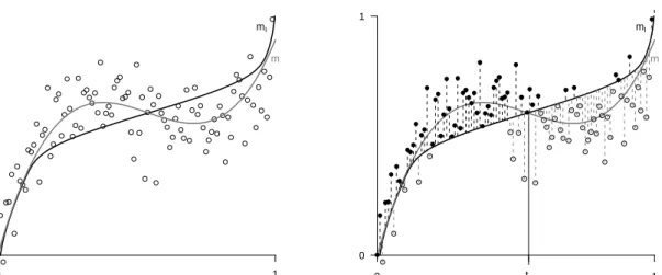
ε1,I, . . . , εn,I behave differently. If the true function m is not monotone (e.g. like in Figure
1) and we calculate the pseudo-residuals frommI too many of them are positive (see solid
dots with black lines) on some subinterval of [0,1] and too many are negative (see open dots with grey lines) on another subinterval. Therefore, they are no longer identically distributed if H0 is not fulfilled.
0 1 0 1 m mI 0 t0 1 0 1 m mI
Figure 1: Left part: True function m (grey line), monotonized function mI (black line)
together with observations. Right part: Pseudo-residuals (positive ones solid with black dashed lines, negative ones open with grey dashed lines)
We construct test statistics from several estimated empirical processes to detect this different behaviour. The first process we will consider is defined as
Sn(t) = 1 √ n n X i=1 I{εˆi,I >0}I{Xi ≤t} − 1 2FˆX,n(t)
where t ∈ [0,1] and ˆFX,n denotes the empirical distribution function of the covariates
X1, . . . , Xn. For every t ∈ [0,1] it counts how many pseudo-residuals are positive up to
covariates ≤t. This term is then centered with respect to the estimated expectation under
H0 and scaled with n−1/2. Under assumptions (A1)–(A5), Sn(t) consistently estimates the
expectation √ nE[I{εi,I >0}I{Xi ≤t}]− 1 2FX(t) = √nE[I{εi >(mI −m)(Xi)}I{Xi ≤t}]−(1−Fε(0))FX(t) (3.3) = √n Z t 0 Fε(0)−Fε((mI −m)(x)) fX(x)dx.
This term is zero for all t ∈ [0,1] if and only if mI = m is valid FX-a. s. To obtain
this equivalence one especially uses that Fε is strictly increasing, whereas equality (3.3)
applies assumption (A5). As we have seen, for instance a Kolmogorov-Smirnov type statistic
sn = supt∈[0,1]|Sn(t)| estimates a distance measure between mI and m and, to obtain a
To avoid assumption (A5) one can alternatively consider the process ˜ Sn(t) = √n 1 n n X i=1 I{εˆi,I >0}I{Xi ≤t} −(1−Fˆε,n(0)) ˆFX,n(t) ,
where ˆFε,n denotes the empirical distribution function of ˆε1, . . . ,εˆn.
The application of tests based on Sn and ˜Sn may not lead to good power in cases where m
and mI are quite similar and the variance is large. Hence it seems sensible to not only take
into account the sign of the estimated pseudo-errors, but also their value, i. e. to consider tests based on 1 n n X i=1 ˆ εi,II{εˆi,I >0}I{Xi ≤t}.
The estimated expectation of this term under H0, i. e. E[εiI{εi > 0}I{Xi ≤ t}] is known
to be √σ
2πFX(t) under assumption (A6), and then can be estimated by
ˆ σ √ 2πFˆX,n(t), where ˆ σ= (n−1Pn
i=1εˆ2i)1/2. This leads to the process
Vn(t) = √ n1 n n X i=1 ˆ εi,II{εˆi,I >0}I{Xi ≤t} − ˆ σ √ 2π ˆ FX,n(t) .
To avoid assumption (A6) one can alternatively consider the process ˜ Vn(t) = √n 1 n n X i=1 ˆ εi,II{εˆi,I >0}I{Xi ≤t} − 1 n n X i=1 ˆ εiI{εˆi >0}FˆX,n(t) .
Lemma 3.1 Tests that for some constant c > 0 reject H0 whenever supt∈[0,1]|Vn(t)| > c
or supt∈[0,1]|V˜n(t)| > c are consistent under assumptions (A1)–(A3),(A6) and (A1)–(A4),
respectively.
Because the proof of this statement requires a longer argumentation we defer it to the appendix.
Now let ˆRi,I denote the fractional rank of ˆεi,I with respect to ˆε1,I, . . . ,εˆn,I, i. e.
ˆ Ri,I = 1 n n X j=1 I{εˆj,I ≤εˆi,I}
and consider the term
1 n n X i=1 ˆ Ri,II{εˆi,I >0}I{Xi ≤t},
which (underH0) estimates the expectation
Eh1 n n X j=1 I{εj ≤εi}I{εi >0}I{Xi ≤t} i = E[Fε(εi)I{εi >0}]FX(t) +o(1) = Z 1 Fε(0) x dx FX(t) +o(1) = 1 2 − (Fε(0))2 2 FX(t) +o(1) = 3 8FX(t) +o(1),
where the last equality holds under assumption (A5). This expectation can be estimated by
3
8FˆX,n(t) under (A5) and by 1
2(1−( ˆFε,n(0)) 2) ˆF
X,n(t) otherwise, which leads to the empirical
processes Rn(t) = 1 √ n n X i=1 ˆ Ri,II{εˆi,I >0}I{Xi ≤t} − 3 8FˆX,n(t) ˜ Rn(t) = 1 √ n n X i=1 ˆ Ri,II{εˆi,I >0}I{Xi ≤t} − 1 2(1−( ˆFε,n(0)) 2) ˆF X,n(t) .
Lemma 3.2 Tests that for some constant c > 0 reject H0 whenever supt∈[0,1]|Rn(t)|> c or
supt∈[0,1]|R˜n(t)|> care consistent under assumptions (A1)–(A5),(A7) and (A1)–(A4),(A7),
respectively.
Again, the proof of this result needs a longer argumentation and is defered to the appendix.
4
Main asymptotic results
In the following theorem we state weak convergence results for the processes defined before. Note that we have to assume a strictly increasing regression function to derive the asymptotic distributions. Nevertheless, the monotone regression estimator ˆmI can also be applied for
monotone regression functions with flat parts, see Dette and Pilz (2006).
Theorem 4.1 Assume that m′ is positive in [0,1].
(i)Under assumptions (A1)–(A5) the processSnconverges weakly inℓ∞([0,1])to a Gaussian
process S with covariance
Cov(S(s), S(t)) = FX(s∧t) 1 4+σ 2f2 ε(0) + 2fε(0)E[ε1I{ε1 ≤0}] = FX(s∧t)( 1 4− 1 2π),
where the last equality holds under the additional assumption (A6).
(ii) Under assumptions (A1)–(A4) the process S˜n converges weakly in ℓ∞([0,1]) to a
Gaus-sian process S˜ with covariance Cov( ˜S(s),S˜(t)) = (FX(s∧t)−FX(s)FX(t)) Fε(0)(1−Fε(0)) +σ2fε2(0) + 2fε(0)E[ε1I{ε1 ≤0}] = (FX(s∧t)−FX(s)FX(t))( 1 4 − 1 2π),
where the last equality holds under the additional assumption (A6).
to a Gaussian process V with covariance Cov(V(s), V(t)) = FX(s∧t)( 1 4 − 1 2π)σ 2 −FX(s)FX(t) σ2 4π.
(iv)Under assumptions (A1)–(A4) the process V˜n converges weakly in ℓ∞([0,1]) to a
Gaus-sian process V˜ with covariance Cov( ˜V(s),V˜(t)) = (FX(s∧t)−FX(s)FX(t)) (2Fε(0)−1)E[ε12I{ε1 ≤0}]−(E[ε1I{ε1 ≤0}])2+σ2(1−Fε(0))2 = (FX(s∧t)−FX(s)FX(t))( 1 4 − 1 2π)σ 2,
where the last equality holds under the additional assumption (A6).
(v) Under assumptions (A1)–(A5) the process Rn converges weakly in ℓ∞([0,1]) to a
Gaus-sian process R with covariance Cov(R(s), R(t)) = (FX(s∧t)−FX(s)FX(t)) 29 192 +σ 2(f ε(0)Fε(0)−E[fε(ε1)I{ε1 >0}])2 + 2E[Fε(ε1)ε1I{ε1 ≤0}](fε(0)Fε(0)−E[fε(ε1)I{ε1 >0}]) + 1 16FX(s)FX(t).
(vi)Under assumptions (A1)–(A4) the process R˜n converges weakly inℓ∞([0,1]) to a
Gaus-sian process R˜ with covariance Cov( ˜R(s),R˜(t)) = (FX(s∧t)−FX(s)FX(t)) E[Fε2(ε1)I{ε1 >0}]−(E[Fε(ε1)I{ε1 >0}])2 +σ2(fε(0)Fε(0) +E[fε(ε1)I{ε1 >0}])2 −2E[Fε(ε1)ε1I{ε1 ≤0}](fε(0)Fε(0) +E[fε(ε1)I{ε1 >0}]) .
The proof is given in the appendix.
Remark 4.2 For a normal regression model, i. e. under assumption (A6) we can obtain
asymptotically distribution free tests, because then sup t∈[0,1]| Sn(t)|= sup s∈(0,1)| Sn(FX−1(s))| converges in distribution to (14 − 1
2π) sups∈[0,1]|W(s)| for a Brownian motion W. Similarly,
supt∈[0,1]|S˜n(t)| converges in distribution to (14−21π) sups∈[0,1]|B(s)|, where B is a Brownian
Remark 4.3 The proposed tests can detect local alternatives of the form
H1,n :m(x) =mI(x) +
∆(x)
√
n ,
where ∆ 6= 0 on an interval in [0,1] of positive length. Consider Sn for simplicity. From
(3.3) we see that the asymptotic expectation ofSn(t) under H1,n is
√ n Z t 0 Fε(0)−Fε((mI −m)(x)) fX(x)dx=fε(0) Z t 0 ∆(x)fX(x)dx+o(1).
With similar arguments as in the proof of Theorem 4.1 one can show that under H1,n,
Sn converges in distribution to the process fε(0)R0t∆(x)fX(x)dx +S(t), t ∈ [0,1]. The
Kolmogorov-Smirnov test statistic supt∈[0,1]|Sn(t)| constructed from Theorem 4.1 detects
H1,n because fε(0) supt∈[0,1]|
Rt
0 ∆(x)fX(x)dx|>0.
Remark 4.4 Assume a heteroscedastic regression model
Yi = m(Xi) +σ(Xi)εi, i= 1, . . . , n,
where Xi and εi are independent, E[ε2i] = 1, E[ε4i] < ∞, the regression function m, error
distributionFε and covariate distributionFX fulfill assumptions as before, whereas the
vari-ance function σ2 is twice continuously differentiable and bounded away from zero. Then
similar tests for monotonicity of the regression function m can be constructed by replacing residuals ˆεi and pseudo-residuals ˆεi,I from before by
ˆ εi = Yi−mˆ(Xi) ˆ σ(Xi) , εˆi,I = Yi−mˆI(Xi) ˆ σ(Xi) ,
where ˆσ2 denotes a Nadaraya-Watson estimator for σ2 with kernel K and bandwidth h
n
based on “observations” (Yi−mˆ(Xi))2. With these changes the same processes as before can
be considered for testingH0. Weak convergence to Gaussian processes can be obtained with
methods as in Akritas and Van Keilegom (2001), where the asymptotic covariances change in comparison to Theorem 4.1 due to the estimation of the variance function.
Remark 4.5 Assume a (homoscedastic) fixed design regression model
Yi = m(xni) +εi, i= 1, . . . , n,
with assumptions as before but with nonrandom covariatesxn1 ≤. . .≤xnn such that there
exists a distribution functionFX with support [0,1] so that FX(xni) = ni, i = 1, . . . , n, and
FX fulfills assumptions as before. Then similar tests for monotonicity of m can be derived
by considering sequential empirical processes. For instance, instead of ˜Snwe would consider
¯ Sn(t) = √n 1 n ⌊nt⌋ X i=1 I{εˆi,I >0} −(1−Fˆε,n(0))t ,
where ⌊nt⌋ is the largest integer ≤ nt. Weak convergence of the processes similar to the results in Theorem 4.1 can be obtained with methods as in Neumeyer and Van Keilegom (2009).
5
Bootstrap method and simulation results
Since the asymptotic distributions of the test statistics still depend on the unknown functions
m and f we use the bootstrap procedures to construct tests based on the above statistics. We build bootstrap observations that fulfill the null hypothesis by defining
Yi∗ = ˆmI(Xi) +ε∗i, i= 1, . . . , n.
Here, under assumption (A6) we can generate the bootstrap errorsε∗
1, . . . , ε∗n by the normal
distributionN(0,σˆ2), where ˆσ2 is the estimated variance from residuals ˆε
1, . . . ,εˆn.
Without assumption (A6) instead we apply a nonparametric smoothed residual bootstrap. To this end, we randomly draw ˜ε∗
i with replacement from centered residuals ˜ε1, . . . ,ε˜n, where
˜
εj = ˆεj−n−1Pnk=1εˆk. Let further adenote a small smoothing parameter and let Z1, . . . , Zn
be independent and standard normally distributed. Then, ε∗
i = ˜ε∗i +aZi, i = 1, . . . , n, are
independent, given the original sampleYn={(Xi, Yi)|i= 1, . . . , n}and have a distribution
function ˜Fn,ε with density
˜ fn,ε(y) = 1 na n X i=1 ϕε˜i−y a .
From the bootstrap observations calculate the constrained and unconstrained regression estimators ˆm∗
I and ˆm∗ and build residuals ˆεi,I = Yi∗ −mˆ∗I(Xi) and ˆε∗i = Yi∗ − mˆ(Xi),
respectively. Let ˆF∗
ε,n denote the empirical distribution function of ˆε∗1, . . . ,εˆ∗n and ˆR∗i,I the
fractional rank of ˆε∗
i,I with respect to ˆε∗1,I, . . . ,εˆ∗n,I. The bootstrap versions of the considered
processes are defined as follows,
Sn∗(t) = √n1 n n X i=1 I{εˆ∗i,I >0}I{Xi ≤t} −(1−F˜ε,n(0)) ˆFX,n(t) ˜ Sn∗(t) = √n1 n n X i=1 I{εˆ∗i,I >0}I{Xi ≤t} −(1−Fˆε,n∗ (0)) ˆFX,n(t) Vn∗(t) = √n1 n n X i=1 ˆ ε∗i,II{εˆ∗i,I >0}I{Xi ≤t} − ˆ σ∗ √ 2πFˆX,n(t) ˜ Vn∗(t) = √n1 n n X i=1 ˆ ε∗i,II{εˆ∗i,I >0}I{Xi ≤t} − 1 n n X i=1 ˆ ε∗iI{εˆ∗i >0}FˆX,n(t) R∗n(t) = √1 n n X i=1 ˆ R∗i,II{εˆ∗i,I >0}I{Xi ≤t} − 1 2(1−( ˜Fε,n(0)) 2) ˆF X,n(t)
40 60 80 100 0.02 0.04 0.06 0.08 0.10 0.12 0.14 n S iz e , σ = 0 . 0 2 5 40 60 80 100 0.01 0.02 0.03 0.04 0.05 0.06 0.07 0.08 n S iz e , σ = 0 . 0 5 40 60 80 100 0.00 0.01 0.02 0.03 0.04 0.05 0.06 n S iz e , σ = 0 . 1 40 60 80 100 0.2 0.4 0.6 0.8 1.0 n P o w e r , σ = 0 . 0 2 5 40 60 80 100 0.2 0.4 0.6 0.8 1.0 n P o w e r , σ = 0 . 0 5 40 60 80 100 0.2 0.4 0.6 0.8 1.0 n P o w e r , σ = 0 . 1
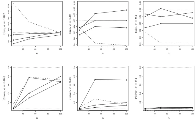
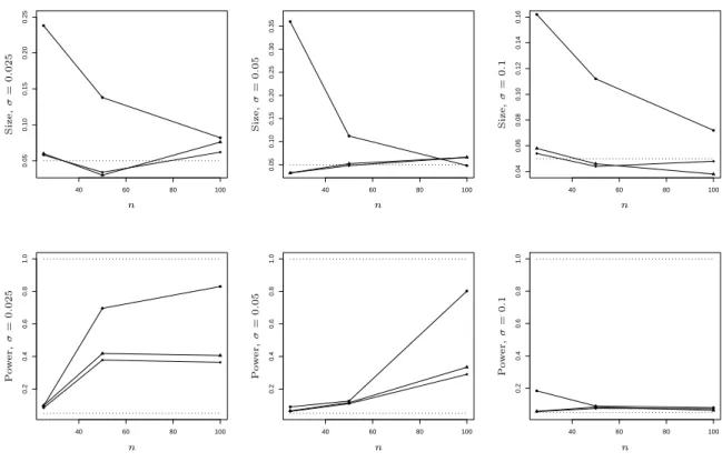
Figure 2: Simulated size and power in dependence of n for the tests ϕsn (diamonds), ϕvn (dots) and ϕrn (triangles) compared to the test ϕL2 (dashed line) for different standard deviations σ (left σ = 0.025, middle σ = 0.05, right σ = 0.1). First row m1, second row
m2,n. ˜ R∗n(t) = √1 n n X i=1 ˆ R∗i,II{εˆ∗i,I >0}I{Xi ≤t} − 1 2(1−( ˆF ∗ ε,n(0))2) ˆFX,n(t) ,
where only in the case ofV∗
n under assumption (A6) we use the parametric bootstrap applying
the normal distribution as explained above, where then ˆσ∗ is the empirical standard deviation
of ˆε∗1, . . . ,εˆ∗n. Note that the bootstrap processes are centered in a slightly different way than
the original statistics with the aim to obtain processes that are asymptotically centered with respect to the conditional expectation E[· | Yn]. In the appendix we sketch a proof for
validity of the bootstrap procedures.
Since it turned out in a simulation study in Birke and Dette (2007), that their test and the test developed by Bowman, Jones and Gijbels (1998) behave very similar we will compare the tests described here only to the one by Birke and Dette (2007). More precisely we use the Kolmogorov-type statistics sn = sup|Sn(t)|, vn = sup|Vn(t)|, rn = sup|Rn(t)|,
˜
sn= sup|S˜n(t)|, ˜vn = sup|V˜n(t)|and ˜rn = sup|R˜n(t)|and denote the corresponding tests by
40 60 80 100 0.02 0.04 0.06 0.08 0.10 0.12 0.14 n S iz e , σ = 0 . 0 2 5 40 60 80 100 0.01 0.02 0.03 0.04 0.05 0.06 0.07 0.08 n S iz e , σ = 0 . 0 5 40 60 80 100 0.00 0.02 0.04 0.06 0.08 n S iz e , σ = 0 . 1 40 60 80 100 0.2 0.4 0.6 0.8 1.0 n P o w e r , σ = 0 . 0 2 5 40 60 80 100 0.2 0.4 0.6 0.8 1.0 n P o w e r , σ = 0 . 0 5 40 60 80 100 0.2 0.4 0.6 0.8 1.0 n P o w e r , σ = 0 . 1
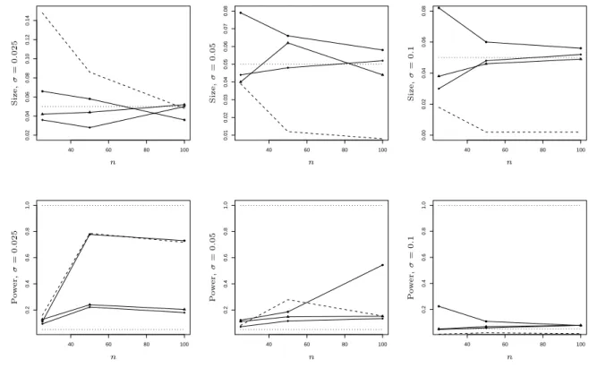
Figure 3: Simulated size and power in dependence of n for the tests ˜ϕsn (diamonds), ˜ϕvn (dots) and ˜ϕrn (triangles) compared to the test ϕL2 (dashed line) for different standard deviations σ (left σ = 0.025, middle σ = 0.05, right σ = 0.1). First row m1, second row
m2,n.
as well as under local alternatives and compare it to the behavior of theL2-testϕ
L2. To this
end we simulate from the regression model
Yi =m(Xi) +σεi
with different regression functions
m1(x) = x, x∈[0,1]
m2,n(x) = x+
1
2√nsin(10πx), x∈[0,1]
and standard normal errors for the sample sizesn = 25, 50 and 100 and standard deviations
σ = 0.025, 0.05 and 0.1. Those errors fulfill all conditions (A4)-(A7) from section 2 and should give acceptable results for all test statistics. We perform 500 simulation runs with each 200 bootstrap repetitions to estimate the size and power of the tests. Note that m1
corresponds to the null hypothesis whilem2,n corresponds to a local alternative as described
40 60 80 100 0.05 0.10 0.15 0.20 0.25 n S iz e , σ = 0 . 0 2 5 40 60 80 100 0.02 0.04 0.06 0.08 0.10 0.12 0.14 n S iz e , σ = 0 . 0 5 40 60 80 100 0.02 0.04 0.06 0.08 0.10 0.12 n S iz e , σ = 0 . 1 40 60 80 100 0.2 0.4 0.6 0.8 1.0 n P o w e r , σ = 0 . 0 2 5 40 60 80 100 0.2 0.4 0.6 0.8 1.0 n P o w e r , σ = 0 . 0 5 40 60 80 100 0.2 0.4 0.6 0.8 1.0 n P o w e r , σ = 0 . 1
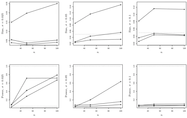
Figure 4: Simulated size and power in dependence of n for the tests ϕsn (diamonds), ϕvn (dots) and ϕrn (triangles) compared to the test ϕL2 (dashed line) for different standard deviationsσ (leftσ = 0.025, middle σ = 0.05, right σ = 0.1) and t-distributed errors. First rowm1, second row m2,n.
1/√n and should therefore be harder to detect by an L2-test than by the empirical process
approach discussed here. The bandwith for the unconstrained estimator is chosen by cross validation while the bandwith for monotonizing is chosen as bn = h1n.2. For generating the
bootstrap data we use a slightly larger bandwidth hn,b =h0n.5 to guarantee the consistency
(see also H¨ardle, 1990 for that). For the smoothed residual bootstrap we use for the test statistics Sn, Rn, ˜Sn, ˜Vn and ˜Rn we need an additional smoothing parameter a which we
choose as a= 0.2ˆσn−0.15.
Figure 2 shows the simulated size (first row) for m1 and the simulated power (second
row) for m2,n of the tests ϕsn, ϕvn and ϕrn. We compare this to the results for the L
2-test
proposed by Birke and Dette (2007) (dashed line). The behavior of the tests heavily depends on the standard deviationσ. For all standard deviations, the tests ϕsn,ϕvn andϕrn are less conservative than the L2-test. Let us now consider the behavior under the alternative. For a small standard deviation (σ = 0.025) all tests behave very similar with some advantages for the L2-test for a sample size of n = 25 and advantages for both the L2-test and the
40 60 80 100 0.05 0.10 0.15 0.20 0.25 n S iz e , σ = 0 . 0 2 5 40 60 80 100 0.05 0.10 0.15 0.20 0.25 0.30 0.35 n S iz e , σ = 0 . 0 5 40 60 80 100 0.04 0.06 0.08 0.10 0.12 0.14 0.16 n S iz e , σ = 0 . 1 40 60 80 100 0.2 0.4 0.6 0.8 1.0 n P o w e r , σ = 0 . 0 2 5 40 60 80 100 0.2 0.4 0.6 0.8 1.0 n P o w e r , σ = 0 . 0 5 40 60 80 100 0.2 0.4 0.6 0.8 1.0 n P o w e r , σ = 0 . 1
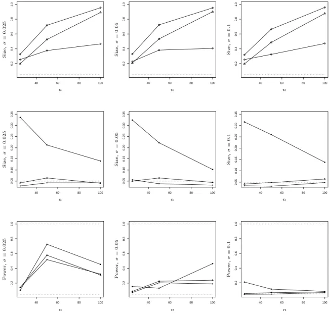
Figure 5: Simulated size and power in dependence of n for the tests ˜ϕsn (diamonds), ˜ϕvn (dots) and ˜ϕrn (triangles) compared to the test ϕL2 (dashed line) for different standard deviationsσ (leftσ = 0.025, middle σ = 0.05, right σ = 0.1) and t-distributed errors. First rowm1, second row m2,n.
test based on Vn for the sample size n = 50. But for n = 100 the power of all tests is
comparable and satisfactorily high for the local alternative. Now, for moderate standard deviation (σ = 0.05) we see clear advantages in the power of the test ϕvn while the results for the tests based onϕsn and ϕrn are still lower than that of theL
2-test. For a comparable
high standard deviation the tests again behave very similar with small advantages for the tests proposed here which have for n = 100 still a power larger than the size of α = 0.05. This is not the case for the L2-test. To conclude the above discussion we note that our assumption in section 3, that ϕvn exhibits the best power, is confirmed for this simulation example.
We already mentioned in section 3, that ϕsn, ϕvn and ϕrn need the restrictive assumption (A5). Furthermore an asymptotic consideration of Vn additionally needs the assumption
(A6) of normal errors and we therefore used the parametric bootstrap in this case. It would now be interesting to see how the more general test statistics behave for the same simulation setting. The results are shown in Figure 3. As before we see that the tests ˜ϕsn, ˜ϕvn and ˜ϕrn
approximate the size better than theL2-test and are therefore less conservative. The behavoir under local alternatives is similar to that of the testsϕsn,ϕvn andϕrn. Again the test ˜ϕvn has the best power under the tests ˜ϕsn, ˜ϕvn and ˜ϕrn. But the different standardisation without using assumption (A5) seems to result in a slightly lower power.
To show the limits concerning the different types of error distributions of the different test statistics, we simulate from the same regression models but now with the following two error distributions
(i) The errors are generated asεi = p
6/8σti,i= 1, . . . , nwhereti,i= 1, . . . , nare drawn
independently from a t-distribution with 8 degrees of freedom.
(ii) The errors are generated asεi =σ(ei−1),i= 1, . . . , nwhereei,i= 1, . . . , nare drawn
independently from an exponential distribution with parameter 1.
(i) Note that in this case, the errors fulfill assumptions (A4), (A5) and (A7) but not (A6) and the expectation is that this choice results in a failure of the test based on Vn since we
need the assumption of normality for deriving the asymptotic distribution while all other test statistics should perform right. Figure 4 shows the results for the tests ϕsn, ϕvn and
ϕrn. As expected we observe, that for m1 and the tests based on ϕsn and ϕrn the size is approximated very well while for the test based on ϕvn, the size is much to large and gets even larger for increasing sample size. Concerning the power of the tests there are no large differences to the case of normal errors. We constructed the further test statistic ˜Vn to avoid
assumption (A6) and therefore the test based on ˜Vn (and, of course, also the tests based
on ˜Sn and ˜Rn) should perform better for those errors. The results are shown in Figure 5.
We observe, that the test ˜ϕvn still has problems to approximate the size for small sample sizes but tends to the right size for larger sample sizes and has the best power of the three different tests. The tests based on ˜ϕsn and ˜ϕrn perform very well with the typical effect that the power gets lower the larger the standard deviation is.
(ii) The centered exponential errors fulfill assumptions (A4) and (A7) but not (A5) and (A6). Therefore we would expect from the theoretical results that the testsϕsn,ϕvn andϕrn can no longer be used while the tests based on ˜ϕsn, ˜ϕvn and ˜ϕrn still behave well. We see the results in Figure 6 where we show the estimated size for Sn, Vn and Rn in the first row
which is much too large and increasing for all tests. In the second and third row we show the estimated size respectively power of the tests ˜ϕsn, ˜ϕvn and ˜ϕrn. Again, the approximated size of the test ˜ϕvn is too large for small sample sizes but seems to approximate it better for larger sample sizes while the other two tests approximate the size very well. All tests perform satisfactorily concerning the power. Here again ˜ϕvn provides the best power.
40 60 80 100 0.2 0.4 0.6 0.8 1.0 replacements n S iz e , σ = 0 . 0 2 5 40 60 80 100 0.2 0.4 0.6 0.8 1.0 n S iz e , σ = 0 . 0 5 40 60 80 100 0.2 0.4 0.6 0.8 1.0 n S iz e , σ = 0 . 1 40 60 80 100 0.05 0.10 0.15 0.20 0.25 0.30 0.35 n S iz e , σ = 0 . 0 2 5 40 60 80 100 0.05 0.10 0.15 0.20 0.25 0.30 0.35 n S iz e , σ = 0 . 0 5 40 60 80 100 0.05 0.10 0.15 0.20 0.25 0.30 0.35 n S iz e , σ = 0 . 1 40 60 80 100 0.2 0.4 0.6 0.8 1.0 n P o w e r , σ = 0 . 0 2 5 40 60 80 100 0.2 0.4 0.6 0.8 1.0 n P o w e r , σ = 0 . 0 5 40 60 80 100 0.2 0.4 0.6 0.8 1.0 n P o w e r , σ = 0 . 1
Figure 6: Behavior of the tests for different standard deviations σ (left σ = 0.025, middle
σ= 0.05, right σ= 0.1) and exponenial errors. First row: Behavior of the testsϕsn,ϕvn and
ϕrn for m1; second and third row: Behavior of the tests ˜ϕsn, ˜ϕvn and ˜ϕrn for m1 respectively
6
Conclusion
In this paper we have considered the problem of testing for monotonicity of regression functions. We have demonstrated that typical distance based tests, which are popular in goodness-of-fit testing in regression models, are not applicable here. As alternative we sug-gested several non-standard, but intuitive distance based tests constructed from Kolmogorov-Smirnov type statistics of empirical processes of residuals estimated both under the null hypothesis of monotonicity and under the general nonparametric model. We presented the asymptotic distributions as well as the small sample performance of bootstrap versions of the tests. We discussed differences in the behaviours of the various tests and compared with the results of theL2-test proposed in Birke and Dette (2007). We have seen, that all empirical process approaches lead to less conservative testing procedures than does the L2-test while having a comparable power. It turned out, that the power is even better for local alternatives of order 1/√n and relatively large standard deviations. But we also observed, that some of the tests fail for non-normal or non-symmetric error distributions.
It is a topic of current research to investigate whether similar tests can be applied to test for monotonicity of quantile regression curves.
A
Proofs
A.1
Consistency proofs
Proof of Lemma 3.1. To check whether Kolmogorov-Smirnov statistics supt∈[0,1]|Vn(t)|
or supt∈[0,1]|V˜n(t)| can lead to a consistent testing procedure we consider the estimated
expectation of the processes and show, that it is 0 if and only if H0 holds. With mI(x)−
m(x) =δ(x) we have √ nE[εi,II{εi,I >0}I{Xi ≤t}]−E[εi{εi >0}I{Xi ≤t}] = √nE[(εi−δ(Xi))I{εi > δ(Xi)}I{Xi ≤t}]−E[εi{εi >0}I{Xi ≤t}] = √n Z t 0 Z ∞ δ(x) (y−δ(x))fε(y)dy− Z ∞ 0 yfε(y)dy fX(x)dx
the latter expression is 0 for all t∈[0,1] if and only if fX-a.s.
0 = Z ∞ δ(x) (y−δ(x))fε(y)dy− Z ∞ 0 yfε(y)dy = − Z δ(x) 0 yfε(y)dy−δ(x) Z ∞ δ(x) fε(y)dy
= − Z δ(x) 0 yfε(y)dy+δ(x) Z δ(x) 0 fε(y)dy−δ(x)(1−Fε(0)) If we define G(z) = 1 (1−Fε(0)) Z z 0 (z−y)fε(y)dy−z
the above equation is equivalent to G(δ(x)) = 0 fX-a.s. Consistency now follows if we can
show that δ(x) = 0 is the only solution of the above equation. To this end note, that with assumption (A4) ∂ ∂zG(z) = 1 1−Fε(0) Z z 0 fε(y)dy−1 = Fε(z)−Fε(0) 1−Fε(0) − 1<0
and thereforeGis strictly decreasing. Sinceδ(x) = 0 is obviously a solution, this is also the only one. This meansmI =m fX−a.s. which is only the case ifm is increasing. Otherwise
mI and m differ on a set with positive measure. 2
Proof of Lemma 3.2. To prove the consistency of supt∈[0,1]|Rn(t)| or supt∈[0,1]|R˜n(t)| we
again consider the estimated expectation of both processes which should be 0 if and only if
H0 is true. Let again δ(x) =mI(x)−m(x). Both Rn(t) and ˜Rn(t) estimate the expectation
Pε1−δ(X1)≤ε2−δ(X2), ε2 > δ(X2), X2 ≤t −1 2(1−F 2 ε(0)) = Z t 0 Z 1 0 Z IR Fε(y+δ(x)−δ(z))I{y>δ(z)}fε(y)dy− Z IR Fε(y)I{y>0}fε(y)dy fX(x)dxfX(z)dz
and this equals 0 for allt∈[0,1] if and only iffX-a.s.:
1−F2 ε(0) 2 = Z 1 0 Z IR Fε(y+δ(x)−δ(z))I{y>δ(z)}fε(y)dyfX(x)dx (A.1) = Z ∞ 0 Z 1 0 Fε(u+δ(x))fX(x)dxfε(u+δ(z))du=:H(δ(z))
Now assume, that δ(x) takes on different values for some different x∈[0,1]. Then we have positive as well as negative values for δ(z) because it is the difference between mI and m
which have to cross if and only if m is not monotone. For a positive value v of δ(z) the derivative of the function
H(v) = Z ∞ 0 K(u)fε(u+v)du with K(u) =R∞ 0 R1 0 Fε(u+δ(x))fX(x)dxfε(u+v)du is ∂ ∂vH(v) = Z ∞ 0 K(u)fε′(u+v)du <0
for a unimodal density fε centered in 0 (assumptions (A4) and (A7)). That is H is strictly
decreasing for v ∈ [0,∞). This is a contradiction to equation (A.1) which means that H is constant. We conclude, that for some d+ > 0, δ(x+) = d+ for all x+ ∈ I+ = {x ∈ [0,1] |
δ(x) > 0}. Since two different negative values of δ cause two different positive value of δ,
δ(x−) = d− for somed− <0 and for allx− ∈I− ={x∈[0,1]|δ(x)<0}. Becaused+ 6=d−,
δwould have at least one point of discontinuity which is not possible because mI and m are
both continuous functions. Therefore, I+ =I− =∅, which meansδ = 0 fX −a.s. 2
A.2
Auxiliary results
Lemma A.1 Under assumptions (A1)–(A5) under the null hypothesis of an increasing
re-gression function m, it holds that
sup x∈[0,1]| ˆ mI(x)−m(x)| = oP(1), sup x∈[0,1]| ˆ m′I(x)−m′(x)| = oP(1) sup x,t∈[0,1] |mˆ′ I(x)−m′(x)−mˆ′I(t) +m′(t)| |x−t|δ = oP(1).
Proof of Lemma A.1. The first assertion directly follows from Theorem 3.3 in Birke and
Dette (2008). For the second assertion we decompose
|mˆ′I(x)−m′(x)| = 1 ( ˆm−1 I )′( ˆmI(x))− 1 (m−1)′(m(x)) ≤ ( ˆm−I1)′( ˆm I(x))−(m−1)′( ˆmI(x)) ( ˆm−I1)′( ˆmI(x))(m−1)′( ˆmI(x)) + 1 (m−1)′( ˆmI(x)) − 1 (m−1)′(m(x))
and use Theorem 3.3 in Birke and Dette (2008) again and the uniform continuity of (m−1)′.
It remains to establish the Lipschitz condition. To this end we distinguish two different cases where |s−t| > b2
n and |s−t| ≤ bn2 for the sequence of bandwidths hn →0 for n → ∞. In
the first case we derive sup |s−t|>b2 n |mˆ′ I(s)−m′(s)−( ˆm′I(t)−m′(t))| |s−t|δ ≤ 2 sups∈[0,1]|mˆ′ I(s)−m′(s)| b2δ n = OP logh−1 n nh3 nb4nδ 1/2 =oP(1),
see Blondin (2007). In the second case we decompose
Dn(s, t) = |mˆ′I(s)−m′(s)−( ˆm′I(t)−m′(t))| ≤ |mˆ′I(s)−mˆ′I(t)|+|m′(s)−m′(t)| = Dn(1)(s, t) +Dn(2)(s, t), D(1) n (s, t) = | ( ˆm−I1)′( ˆm I(s))−( ˆmI−1)′( ˆmI(t))| ( ˆm−I1)′( ˆmI(s))( ˆm−1 I )′( ˆmI(t))
and define D(1)n = sup |s−t|≤b2 n D(1)n (s, t) |s−t|δ ≤C1 sup |u−v|≤Cb2 n |( ˆm−I1)′(u)−( ˆm−1 I )′(v)| |mˆ−I1(u)−mˆ−I1(v)|δ .
The last inequality follows because ˆmI is continuously differentiable and, hence, Lipschitz
continuous. Under the assumptions (A3) we obtain by using Taylor expansions
|mˆ−I1(u)−mˆ−I1(v)| = 1 bn Z 1 0 km(x)−v bn dx|u−v|(C2+oP(1)) |( ˆm−I1)′(u)−( ˆm−I1)′(v)| = 1 bn k m(1)−v bn −km(0)−v bn |u−v|(C3+oP(1))
That means forD(1)n
Dn(1) ≤ C1 sup |u−v|≤Cb2 n 1 bn k m(1)−v bn −km(0)b −v n |u−v|(C3+oP(1)) 1 bn R1 0 k m(x)−v bn dxδ|u−v|δ(C 2+oP(1)) = OP sup |u−v|≤Cb2 n |u−v|1−δ bn =OP(b1n−2δ) =oP(1).
The regression function m is two times continuously differentiable and therefore m′ is
Lips-chitz continuous on [0,1]. That means sup |s−t|≤b2 n D(2)n (s, t) |s−t|δ =O(b 2−2δ n ) = o(1). 2
Lemma A.2 Under assumptions (A1)–(A5) under the null hypothesis of an increasing
re-gression function m, it holds that
Z t 0 ( ˆmI(x)−mˆ(x))fX(x)dx = oP( 1 √ n)
uniformly with respect to t∈[0,1].
Proof of Lemma A.2. We use the representation
ˆ
mI(x)−m(x) = −
ˆ
m−I1−m−1
(m−1)′ (m(x)) + ˜Bn(x)
(see Birke and Dette, 2008) with ˜ Bn(x) = ( ˆm−I1(m(x))−m−1(m(x))) 1 (m−1)′(m(x)) − 1 ˆ m−I1(ηn(x))
and |ηn(x)−m(x)| ≤ |mˆI(x)−m(x)| for all x to rewrite Z t 0 ( ˆmI(x)−m(x))fX(x)dx = − Z m(t) m(0) ( ˆm−I1(u)−m−1(u))fX(m−1(u))du+ Z t 0 ˜ Bn(x)dx = An(t) +Bn(t), where An(t) = An,1(t) +An,2(t) +An,3(t) (A.2) and An,1(t) = − Z t 0 (mI(x)−m(x))fX(x)dx= 0 An,2(t) = − 1 bn Z 1 0 Z m(t) m(0) km(v)−u bn fX(m−1(u))du( ˆm(v)−m(v))dv An,3(t) = − 1 bn Z 1 0 Z m(t) m(0) k′ξ(v)−u bn fX(m−1(u))du( ˆm(v)−m(v))2dv.
One obtains the expansion
An,2(t) = Z t 0 ( ˆm(v)−m(v))fX(v)dv− Z m−1(m(0)+b n) 0 ( ˆm(v)−m(v))fX(v)dv − Z m−1(m(t)−bn) m−1(m(0)+bn) ( ˆm(v)−m(v))fX(v)dv (1 +oP(b2n)) = Z t 0 ( ˆm(v)−m(v))fX(v)dv−Rn,1(t)−Rn,2(t) (1 +oP(b2n)).
The two remainders Rn,1(t) and Rn,2(t) can be handled in the same way. We show the
estimation ofRn,1(t) here. Rn,1(t) ≤ sup|mˆ(v)−m(v)|supfX(v)m−1(m(0) +bn) =OP b2 nlogh−n1 nhn 1/2 =oP 1 √ n sinceb2
nlogh−n1/hn→0. The third termAn,3(t) in the decomposition (A.2) can be estimated
by similar means as ∆(2)n in Dette, Neumeyer and Pilz (2006) as
An,3(t) = OP 1 nhn =oP 1 √ n ,
the first one as An,1(t) = O(b2n) = o(1/
√ n) and Z t 0 ˜ Bn(x)dx=oP 1 √ n
by using similar arguments as for estimating the deterministic part andBn,j(x) in Birke and
Dette (2007). This means
Z t 0 ( ˆmI(x)−m(x))fX(x)dx= Z t 0 ( ˆm(x)−m(x))fX(x)dx+oP 1 √ n .
wich proves the assertion. 2
Lemma A.3 Under assumptions (A1)–(A5) under the null hypothesis of an increasing
re-gression function m, it holds that
Z t 0 ( ˆm(x)−m(x))fX(x)dx = 1 n n X i=1 εiI{Xi ≤t}+oP( 1 √ n)
uniformly with respect to t∈[0,1].
Proof of Lemma A.3. From the proof of Proposition 2.10 by Neumeyer and Van Keilegom
(2009) it follows that Z t 0 ( ˆm(x)−m(x))fX(x)dx = 1 n n X i=1 εi Z t 0 1 hn KXi−x hn dx+oP( 1 √ n)
uniformly with respect tot∈[0,1]. Applying Theorem 2.11.23 in Van der Vaart and Wellner (1996, p. 221) (similar to, but simpler than the proof of Th. 2.7 in the aforementioned paper) one shows that the process
1 √ n n X i=1 εi I{Xi ≤t} − Z t 0 1 hn KXi−x hn dx, t ∈[0,1],
converges weakly to a degenerated Gaussian process with vanishing covariances. This proves the assertion. 2
A.3
Proof of main results
Proof of Theorem 4.1.
(i). The process Sn has the following simple form,
Sn(t) = √ n1 n n X i=1 I{Xi ≤t} − 1 n n X i=1 I{εˆi,I ≤0}I{Xi ≤t} − 1 2FˆX,n(t) = √n1 2FˆX,n(t)−FˆX,εI,n(t,0) (A.3)
where ˆFX,εI,n denotes the empirical distribution function of (Xi,εˆi,I), i= 1, . . . , n. Further let FX,ε,n denote the empirical distribution function of (Xi, εi), i = 1, . . . , n. Analogous to
the proof of Lemma A.2 in Neumeyer and Van Keilegom (2009) applying Lemma A.1 it holds that ˆ FX,εI,n(t, y) = FX,ε,n(t, y) +fε(y) Z t 0 ( ˆmI(x)−m(x))fX(x)dx+oP( 1 √ n)
uniformly with respect to t ∈ [0,1] and y ∈ IR. Applying Lemma A.2 and (A.3) it follows that ˆ FX,εI,n(t, y) = 1 n n X i=1 I{Xi ≤t}I{εi ≤y}+fε(y) 1 n n X i=1 εiI{Xi ≤t}+oP( 1 √ n) (A.4) and Sn(t) = 1 √ n n X i=1 I{Xi ≤t} 1 2 −I{εi ≤0} −εifε(0) +oP(1)
uniformly with respect tot ∈[0,1]. Weak convergence to the asserted Gaussian process now follows by standard arguments. 2
(ii). The proof for ˜Sn is very similar to (i). We have
˜ Sn(t) = √n 1 n n X i=1 I{Xi ≤t} − 1 n n X i=1 I{εˆi,I ≤0}I{Xi ≤t} −(1−Fˆε,n(0)) ˆFX,n(t) = √n−FˆX,εI,n(t,0) + ˆFε,n(0) ˆFX,n(t)
Similarly to (A.4) one has ˆ Fε,n(y) = 1 n n X i=1 I{εi ≤y}+fε(y) 1 n n X i=1 εi+oP( 1 √ n) (A.5)
(this follows from Akritas and Van Keilegom (2001), see also Neumeyer and Van Keilegom (2009), for instance). Applying (A.4) and (A.5) we obtain the expansion
˜ Sn(t) = 1 √ n n X i=1 ˆ FX,n(t)−I{Xi ≤t} I{εi ≤0}+εifε(0) +oP(1) = √1 n n X i=1 FX(t)−I{Xi ≤t} I{εi ≤0}+εifε(0) +√n( ˆFX,n(t)−FX(t))(Fε(0) +oP(1)) +oP(1) = √1 n n X i=1 I{Xi ≤t} −FX(t) Fε(0)−I{εi ≤0} −εifε(0) +oP(1)
uniformly with respect to t ∈ [0,1]. Weak convergence to a Gaussian process with the asserted covariance structure follows by standard arguments. 2
(iii). From Lemma A.1 it follows that P(m−mˆI ∈ C) → 1 for n → ∞, where the class
C =C11+δ[0,1] of smooth functions is defined in Van der Vaart and Wellner (1996, p. 154),
and its bracketing number fulfills
logN[ ](ǫ,C,|| · ||∞) ≤ Kǫ−1/(1+δ)
for some K > 0 and all ǫ >0, where || · ||∞ denotes the supremum norm (see Th. 2.7.1 in
the same reference). Note that for the process ¯ Vn(t, h) = 1 n n X i=1 (εi+h(Xi))I{εi+h(Xi)>0}I{Xi ≤t}, t ∈[0,1], h∈ C, we have ¯ Vn(t, m−mˆI) = 1 n n X i=1 ˆ εi,II{εˆi,I >0}I{Xi ≤t}
(compare to the definition ofVn). Now consider the empirical process
√ n( ¯Vn(t, h)−E[ ¯Vn(t, h)]) = 1 √ n n X i=1 gh,t(Xi, εi)−E[gh,t(Xi, εi)] ,
where the functions gh,t vary over the pairwise products of the function classes G and H
defined as G = nε 7→(ε+h(x))I{ε+h(x)>0} g ∈ C o H = nx7→I{x≤t} t∈[0,1] o .
H is Donsker by standard empirical process theory with bracketing numbers N[ ](ǫ,H,|| ·
||∞) = O(ǫ−1). In the following we calculate bracketing numbers for G. Let ǫ > 0 and
let [hL
j, hUj ] (j = 1, . . . , m) build ǫ2-brackets for C, where m = N[ ](ǫ2,C,|| · ||∞). Then for hL
j ≤h≤hUj one has
(ε+hLj(x))I{ε+hjL(x)>0} ≤(ε+h(x))I{ε+h(x)>0} ≤(ε+hUj (x))I{ε+hUj (x)>0} and such a bracket hasL2-length
Eh(ε1 +hUj (X1))I{ε1+hUj (X1)>0} −(ε1+hLj(X1))I{ε1+hLj(X1)>0} 2i1/2 ≤ 2Eh(|ε1|+ 1)2(I{ε1+hUj (X1)>0} −I{ε1 +hLj(X1)>0})2+ (hUj (X1)−hLj(X1))2 i1/2 ≤ 2 Z Z −hLj(x) −hU j(x) (|y|+ 1)2fε(y)dy fX(x)dx+ 4||hUj −hLj||∞ 1/2 ≤ 2||hUj −hLj||∞E[(|ε1|+ 1)2] + 4||hUj −hLj||∞ 1/2 ≤ cǫ
for some constantc, where we have used that |hLj| ≤1, |hUj| ≤1.
The function classHGof pairwise products has a square-integrable envelope and the covering numbers with respect to theL2-norm || · ||2 fulfill
logN[ ](ǫ,HG,|| · ||2) ≤ log N[ ](ǫ,G,|| · ||2)N[ ](ǫ,H,|| · ||2) ≤ c1log N[ ](c2ǫ2,C,|| · ||∞)N[ ](ǫ,H,|| · ||2) ≤ c3log(exp(ǫ−2/(1+δ))ǫ−1)
for some constants c1, c2, c3, for ǫ ≤ 2(E[(|ε1|+ 1)2])1/2, whereas for larger ǫ one bracket is
sufficient, because
|(ε+h(x))I{ε+h(x)>0}I{x≤t}| ≤ |ε|+ 1 for all h∈ C, t∈[0,1]. Hence,
Z ∞ 0 logN[ ](ǫ,HG,|| · ||2) 1/2 dǫ < ∞
and GH is Donsker [see Van der Vaart and Wellner (1996, p. 129)]. This yields weak convergence of the empirical process
ˇ Vn(h, t) = 1 √ n n X i=1 n (εi+h(Xi))I{εi+h(Xi)>0} −εiI{εi >0} I{Xi ≤t} −Eh(ε1+h(X1))I{ε1+h(X1)>0} −ε1I{ε1 >0} I{X1 ≤t} i o , t∈[0,1], h∈ C, to a Gaussian process. For the expectation we obtain the expansion
Eh(ε1+h(X1))I{ε1+h(X1)>0} −ε1I{ε1 >0} I{X1 ≤t} i = Z Z (y+h(x))I{y+h(x)>0}I{x≤t}fX(x)fε(y)dxdy −FX(t) Z yI{y >0}fε(y)dy = Z Z zI{z >0}I{x≤t}fX(x)(fε(z−h(x))−fε(z))dxdz (A.6)
which tend to zero if supx∈[0,1]|h(x)| → 0. Similarly it follows that the covariances
Cov( ˇVn(h, s),Vˇn(h, t)) tend to zero if supx∈[0,1]|h(x)| →0. Hence, with Van der Vaart (1998,
Le. 19.24 and proof of Le. 19.26, p. 280) we obtain that supt∈[0,1]|Vˇn(m−mˆI, t)|=oP(1).
Inserting h = m−mˆI into (A.6) for the expectation and applying Taylor’s expansion we
obtain
Z Z
= Z Z zI{z >0}I{x≤t}fX(x)fε′(z)( ˆmI(x)−m(x))dxdz+oP( 1 √ n) = Z ∞ 0 zfε′(z)dz Z t 0 ( ˆmI(x)−m(x))fX(x)dx+oP( 1 √ n) = (Fε(0)−1) 1 n n X i=1 εiI{Xi ≤t}+oP( 1 √ n),
where the last equality follows from integration by parts and Lemmata A.2 and A.3. Combining all results we obtain the asymptotic expansion
1 √ n n X i=1 ˆ εi,II{εˆi,I >0}I{Xi ≤t} (A.7) = √1 n n X i=1 εi I{εi >0} −(1−Fε(0)) I{Xi ≤t}+oP(1).
For the asymptotic expansion ofVnnow consider ˆσ−σ= (ˆσ2−σ2)/(ˆσ+σ) = (ˆσ2−σ2)/2σ+
oP(1/√n), from which with results by M¨uller, Schick and Wefelmeyer (2004) it follows that
ˆ σ−σ = 1 2σn n X i=1 (ε2i −σ2) +oP( 1 √ n) and ˆ σ √ 2π ˆ FX,n(t) = 1 2√2πσn n X i=1 (ε2i −σ2)FX(t) + σ √ 2π 1 n n X i=1 (I{Xi ≤t} −FX(t)) +√σ 2πFX(t) +oP( 1 √ n). Now we have Vn(t) = 1 √ n n X i=1 εiI{εi >0}I{Xi ≤t} − σ √ 2πFX(t)−εi(1−Fε(0))I{Xi ≤t} −(ε2i −σ2) FX(t) 2√2πσ − σ √ 2π(I{Xi ≤t} −FX(t)) +oP(1) = √1 n n X i=1 εiI{εi >0} − σ √ 2π − 1 2εi I{Xi ≤t} −(ε2i −σ2) FX(t) √ 8πσ +oP(1)
The proof of weak convergence is omitted for the sake of brevity. The calculation of the covariances uses that under (A6),
E[ε1I{ε1 >0}] = σ √ 2π, E[ε 2 1I{ε1 >0}] = σ2 2 , E[ε 3 1I{ε1 >0}] = 2σ3 √ 2π. 2
(iv). We only give a sketch of the asymptotic expansion for the process ˜Vn. Similarly to
(A.7) one obtains 1 √ n n X i=1 ˆ εiI{εˆi >0}FˆX,n(t) = √1 n n X i=1 εi I{εi >0} −(1−Fε(0)) ˆ FX,n(t) +oP(1) = √1 n n X i=1 εi I{εi >0} −(1−Fε(0)) FX(t) − √1 n n X i=1 (I{Xi ≤t} −FX(t)) E[ε1I{ε1 >0}] +oP(1) +oP(1)
and in combination with (A.7) this yields the expansion ˜ Vn(t) = 1 √ n n X i=1 εiI{εi >0} −E[ε1I{ε1 >0}]−εi(1−Fε(0)) I{Xi ≤t} −FX(t) +oP(1). 2
(v). We first consider the process ¯ Rn(t) = 1 √ n n X i=1 ˆ Ri,II{εˆi,I >0}I{Xi ≤t},
where ˆRi,I = ˆFX,εI,n(0,εˆi,I). On has the expansion ¯Rn= ¯R1,n+ ¯R2,n, where ¯ R1,n(t) = 1 √ n n X i=1 Fε(ˆεi,I)I{εˆi,I >0}I{Xi ≤t} ¯ R2,n(t) = 1 √ n n X i=1 ˆ FX,εI,n(1,εˆi,I)−Fε(ˆεi,I) I{εˆi,I >0}I{Xi ≤t}.
Analogously to the proof of (iii) [see (A.7)] we obtain ¯ R1,n(t) = 1 √ n n X i=1 Fε(εi)I{εi >0}I{Xi ≤t} +√n Z fε′(z)Fε(z)I{z >0}dz Z t 0 ( ˆmI(x)−m(x))fX(x)dx+oP(1) = √1 n n X i=1 Fε(εi)I{εi >0} −εi fε(0)Fε(0) +E[fε(ε1)I{ε1 >0}] I{Xi ≤t}+oP(1).
Now, for the second term we have ¯ R2,n(t) = √n Z Z ˆ FX,εI,n(1, y)−Fε(y) I{y >0}I{x≤t}dFX(x)dFε(y) +√n Z ( ˆFX,εI,n−FX ⊗Fε)(1, y)I{y >0}I{x≤t}d( ˆFX,εI,n−FX ⊗Fε)(x, y). The last integral converges to zero uniformly in probability, because the process√n( ˆFX,εI,n−
FX⊗Fε) converges to a Gaussian process, see the proof of (i). Inserting the expansion (A.4)
we further have ¯ R2,n(t) = 1 √ n n X i=1 Z I{εi ≤y} −Fε(y) +fε(y)εi I{y >0}dFε(y)FX(t) +oP(1) = √1 n n X i=1 1−Fε(0) +I{εi >0}(Fε(0)−Fε(εi))−E[Fε(ε1)I{ε1 >0}] +εiE[fε(ε1)I{ε1 >0}] FX(t) +oP(1).
We obtain the expansion
Rn(t) = ¯R1,n(t) + ¯R2,n(t)−E[Fε(ε1)I{ε1 >0}] 1 √ n n X i=1 I{Xi ≤t} = √1 n n X i=1 I{Xi ≤t} −FX(t) Fε(εi)I{εi >0} −E[Fε(ε1)I{ε1 >0}] +εi fε(0)Fε(0)−E[fε(ε1)I{ε1 >0}] +1−Fε(0) +I{εi >0}Fε(0)−2E[Fε(ε1)I{ε1 >0}] FX(t) +oP(1). 2
(vi). With (A.5) one obtains
ˆ Fε,n2 (0) = 2Fε(0) n n X i=1 (I{εi ≤0}+fε(0)εi)−Fε2(0) +oP( 1 √ n). Further we have 1 2(1−Fˆ 2 ε,n(0)) ˆFX(t) = 1 2 ˆ FX(t)−Fˆε,n2 (0)FX(t)−Fε2(0)( ˆFX(t)−FX(t)) +oP( 1 √ n) = 1 n n X i=1 1 2(1−F 2 ε(0))I{Xi ≤t} −FX(t)Fε(0)(I{εi ≤0}+fε(0)εi) +Fε2(0)FX(t) +oP( 1 √ n),
and hence, with notations from the proof of (v), ˜ Rn(t) = ¯R1,n(t) + ¯R2,n(t)− √ n 2 (1−Fˆ 2 ε,n(0)) ˆFX(t) = √1 n n X i=1 (I{Xi ≤t} −FX(t)) Fε(εi)I{εi >0} −E[Fε(ε1)I{ε1 >0}] −εi(fε(0)Fε(0) +E[fε(ε1)I{ε1 >0}]) +oP(1). 2
A.4
Validity of bootstrap
In the following we sketch the proof of bootstrap consistency for the process ˜
Sn∗(t) = √n−FˆX,ε∗ I,n(t,0) + ˆFε,n∗ (0) ˆFX,n(t)
(the other processes are treated similarly). From Neumeyer (2009, Lemma 2) (confer this reference also for restrictions on the bandwidth a) we have
ˆ Fε,n∗ (y) = 1 n n X i=1 I{ε∗i ≤y}+ ˜fε,n(y) 1 n n X i=1 ε∗i +oP( 1 √ n).
Combining the methods shown in the paper at hand with the methods by Neumeyer (2009) one can show similarly to (A.4) that
ˆ FX,ε∗ I,n(t, y) = 1 n n X i=1 I{Xi ≤t}I{ε∗i ≤y}+ ˜fε,n(y) 1 n n X i=1 ε∗iI{Xi ≤t}+oP( 1 √ n).
Hence we obtain the expansion ˜S∗
n(t) = ˜Sn∗,1(t) +oP(1), where ˜ Sn∗,1(t) = √1 n n X i=1 ˆ FX,n(t)−I{Xi ≤t} I{ε∗i ≤0} −F˜ε,n(0) +ε∗if˜ε,n(0)
uniformly with respect tot ∈[0,1]. Note that bootstrap results are formulated conditionally on the original sample Yn = {(Xi, Yi) | i = 1, . . . , n} and hence, that in this expansion
ˆ
FX,n and ˜Fε,n,f˜ε,n are “not random”. Further, for the conditional expectation we have
E[ ˜S∗,1
n (t)| Yn] = 0. To derive weak convergence we first consider the conditional covariances
Cov( ˜Sn∗,1(t),S˜n∗,1(s)| Yn) = ˆ FX,n(s∧t)−FˆX,n(s) ˆFX,n(t) ˜ Fε,n(0)(1−F˜ε,n(0)) + ˜fε,n2 (0) Z y2f˜ε,n(y)dy+ 2 ˜fε,n(0) Z yI{y≤0}f˜ε,n(y)dy ,
which (under regularity conditions) converge almost surely to Cov( ˜S(t),S˜(s)) as defined in Theorem 4.1.
Using Cram´er-Wold’s device and Lindeberg’s condition one can show convergence of the finite dimensional distributions analogously to the proof of Theorem 3 by Neumeyer (2009). To show tightness we follow the proof of Lemma A.3 by Stute, Gonz´alez Manteiga and Presedo Quindimil (1998). To this end, note that the dominating term of the process has the form ˜ Sn∗,1(t) = √1 n n X i=1 ˆ FX,n(t)−I{Xi ≤t} Zn,i∗ where E[Z∗
n,i | Yn] = 0 and E[(Zn,i∗ )4 | Yn] is independent of i and converges for n → ∞to
positive constants with probability one. For 0 ≤ s ≤ t ≤ r ≤ 1 one can easily obtain the bound EhS˜n∗,1(t)−S˜n∗,1(s) ˜ Sn∗,1(r)−S˜n∗,1(t) Yn i ≤ CFˆX,n(r)−FˆX,n(s) 2 E[(Zn,i∗ )4 | Yn]
for some constantC. Tightness follows as in the aforementioned proof from monotonicity of ˆ
FX,n, which converges almost surely to FX.
Altogether we obtain that the process ˜S∗
n, conditional onYn converges weakly to the process
˜
S as defined in Theorem 4.1, in probability. 2
Acknowledgements. The authors would like to thank Birte Muhsal for generating Figure
1. This work has been supported in part by the Collaborative Research Center ”Statistical modeling of nonlinear dynamic processes” (SFB 823) of the German Research Foundation (DFG).
B
References
M. Akritas, I. Van Keilegom (2001). Nonparametric estimation of the residual
distri-bution. Scand. J. Statist. 28, 549–567.
Y. Baraud, S. Huet and B. Laurent (2003). Adaptive tests of qualitative hypotheses
ESAIM, Probab. Statist. 7, 147–159.
M. Birke and H. Dette (2007). Testing strict monotonicity in nonparametric regression.
Math. Meth. Statist. 16, p. 110–123.
M. Birke and H. Dette (2008). A note on estimating a smooth monotone regression by
combining kernel and density estimates. J. Nonparam. Statist. 20, 679–691.
D. Blondin (2007). Rates of strong uniform consistency for local least squares kernel
A. W. Bowman, M. C. Jones and I. Gijbels (1998). Testing monotonicity of regres-sion. J. Computational and Graphical Statist. 7, 489–500.
H. Dette, N. Neumeyer and K. F. Pilz (2006). A simple nonparametric estimator of a
strictly monotone regression function. Bernoulli 12 , 469–490.
H. Dette and K. F. Pilz (2006). A comparative study of monotone nonparametric kernel
estimates. J. Stat. Comput. Simul. 76, 41–56.
J. Dom´ınguez-Menchero, G. Gonz´alez-Rodr´ıguez and M. J. L´opez-Palomo (2005).
An L2 point of view in testing monotone regression J. Nonparam. Statist. 17, 135–153.
L. D¨umbgen (2002). Application of local rank tests to nonparametric regression. J.
Non-parametr. Stat. 14, 511–537.
C. Durot (2003). A Kolmogorov-type test for monotonicity of regression. Statist. Probab.
Lett. 63, 425–433.
I. Gijbels (2005). Monotone regression. In N. Balakrishnan, S. Kotz, C.B. Read and B.
Vadakovic (eds), The Encyclopedia of Statistical Sciences, 2nd edition. Hoboken, NJ: Wiley.
I. Gijbels, P. Hall, M. C. Jones and I. Koch (2000). Tests for monotonicity of a
re-gression mean with guaranteed level. Biometrika 87, 663–673.
S. Ghosal, A. Sen, A. W. van der Vaart (2000). Testing monotonicity of regression.
Ann. Statist. 28, 1054–1082.
P. Hall and N. E. Heckman (2000). Testing for monotonicity of a regression mean by
calibrating for linear functions. Ann. Statist. 28, 20–39.
P. Hall and L.-S. Huang (2001). Nonparametric kernel regression subject to
monotonic-ity constraints. Ann. Statist. 29, 624–647.
W. H¨ardle (1990). Applied nonparametric regression. Cambridge Univ. Press.,
Cam-bridge
W. H¨ardle and E. Mammen (1993). Comparing nonparametric versus parametric
regression fits. Ann. Statist. 21, 1926–1947.
Hardy, G.H., Littlewood, J.E. and P´olya, G. (1952). Inequalities. 2nd ed.,
Lieb, E.H. and Loss, M. (2001). Analysis. 2nd ed., Graduate Studies in Mathematics. 14. Providence, RI: American Mathematical Society
E. Mammen (1991). Estimating a smooth monotone regression function. Ann. Statist.
19, 724–740.
U. U. M¨uller, A. Schick, W. Wefelmeyer (2004). Estimating linear functionals of the
error distribution in nonparametric regression. J. Statist. Plann. Inference 119, 75–93.
N. Neumeyer (2009). Smooth residual bootstrap for empirical processes of nonparametric
regression residuals. Scand. J. Statist. 36, 204–228.
N. Neumeyer and I. Van Keilegom (2009). Changepoint tests for the error distribution
in nonparametric regression. Scand. J. Statist. 36, 518 - 541.
W. Schlee (1982). Nonparametric tests of the monotony and convexity of regression.
Non-parametric statistical inference, Vol. I, II, 823–836, Colloq. Math. Soc. J´anos Bolyai, 32, North-Holland, Amsterdam.
B. W. Silverman (1981). Using kernel density estimates to investigate multimodality. J.
Roy. Statist. Soc. Ser. B 43, 97–99.
W. Stute (1997). Nonparametric model checks for regression. Ann. Statist. 25, 613–641.
W. Stute, W. Gonz´alez Manteiga and M. Presedo Quindimil (1998). Bootstrap
Approximation in Model Checks for Regression. J. Amer. Statist. Assoc. 93, 141–149.
A. W. Van der Vaart (1998). Asymptotic statistics. Cambridge University Press,
Cam-bridge.
A. W. Van der Vaart and J. A. Wellner (1996). Weak convergence and empirical
pro-cesses. Springer, New York.
I. Van Keilegom, W. Gonz´alez–Manteiga and C. S´anchez Sellero (2008).
Goodness-of-fit tests in parametric regression based on the estimation of the error distribution.