New Algorithms and Analysis Techniques for Reinforcement Learning

(1)

Randy Jia

Submitted in partial fulfillment of the requirements for the degree of

Doctor of Philosophy under the Executive Committee of the Graduate School of Arts and Sciences

COLUMBIA UNIVERSITY

(2)

(3)

Abstract

New Algorithms and Analysis Techniques for Reinforcement Learning Randy Jia

In the advent of Big Data and Machine Learning, there is a demand for improved decision making in unknown, complex environments. Decision making under uncertainty is a common principle underlying many important decisions made by individuals, businesses, and society as a whole. These problems are typically modeled as multi-armed bandits (MAB), or, more generally, reinforcement learning (RL). In the MAB problem, an agent is faced with many options or arms, each with its own unknown reward distribution, and must determine the sequence of arms to pull, taking into account history of rewards of past pulls. The agent must balance exploration (pulling less-explored arms to learn the model), with exploitation (pulling the current reward maximizing arm so far). RL is a generalized, more complex extension of the MAB problem in which the current state, in addition to the arm or action, impacts the obtained reward. In this thesis, we focus on designing new algorithms to better address RL problems. In particular, we design an algorithm inspired by Thompson sampling for finite communicating MDPs and an algorithm inspired by stochastic convex optimization for some fundamental problems in operations management, including a problem in inventory control. We develop intuitive algorithms and prove theoretical bounds on their regret; in doing so, we derive some theoretically interesting analytical results that may be of independent interest.

(4)

List of Figures

2.1 Chain MDP withSstates and two actions. . . 30 2.2 Average cumulative regret for chain MDPs withS = 10,15,20,25andT = 100,000. 31 2.3 Very long horizonT = 1,000,000 we can see that UCRL2 begins to learn while

TSRL with 1 samples still does not. . . 32 3.1 Timing of arrival of orders and demand at timet. . . 39 3.2 G/GI/m queue . . . 61

(8)

Acknowledgements

It feels like a long time since I first arrived at Columbia. I remember throughout my first semester many of my colleagues and I wondered if we were in the right place, and whether we would even make it to the end. Now that I have made it, I can definitely say it is all thanks to the many people in my life who have helped me throughout few years.

First and foremost, I want to thank my advisor, Shipra. Shipra has been my advisor ever since Spring of 2016, and it has been a joy working with her these past four years. She has introduced me to this intriguing field of study, guided me through the ups and downs of research, and helped me become the researcher I am today. I cannot thank her enough for her patience, guidance, and support throughout these years. I learned so much: how to approach problems, how to write, how to give talks, how to deal with adversity, the list is endless. I would definitely not have made it here without the tireless effort she has put forth helping me.

I would like to thank the other members of my committee, Vineet, Dan, Garud, and Adam, for their helpful and valuable feedback. I also would like to thank the professors that taught me in my first year core courses: Don, Jose, David, and Cliff. I was challenged to my limits and learned a great deal in a very short span of time, setting me up for success the rest of my time here.

The IEOR staff members tirelessly work to ensure everything runs smoothly for us, and I am truly grateful to Liz, Kristen, Shi Yee, Jaya, Yosimir, and Carmen for everything they have done. I also am thankful for the many great students and colleagues with whom I’ve spent countless hours working, eating, and talking with. Wenbo, Allen, Ryan, Xingyu, Raghav, KG, Min, Vlada, Li, Shuoguang, Jack, Steven, Apurv, Mike, Rajan, Irene, Chun, Suraj, Chen Chen,

(9)

and everyone else I had the honor to be colleagues with, thank you for being there and making the past few years enjoyable.

Thank you Roger for your support and for, as usual, paving the way so your little brother has it easier his time around. Thank you mom and dad for always thinking of me and supporting me, no matter what I decide to do. Finally, thank you Cecilia for being with me almost every step of this journey of mine, from when we met (the day before my Stoch II midterm), to now, your never-ending support has always kept me striving towards success.

(10)

Dedication

(11)

Chapter 1: Introduction

In this dissertation we study new algorithms for decision making problems under uncertainty, a common principle underlying many important decisions made each and every day. How should businesses price and stock products? How should advertisers decide which ads to show, and when? How can healthcare professionals most effectively run a clinical trial for new experimental drugs? These are some practical questions that motivate this complex area of research. The goal is to design new algorithms and analysis techniques that contribute towards a better understanding of solving these types of problems.

These problems are typically modeled as multi-armed bandit (MAB) or reinforcement learning (RL) problems. They both refer to the problem of learning and planning in sequential decision making systems when the underlying system dynamics are unknown, and may need to be learned by trying out different options and observing their outcomes. In the MAB problem, an agent is faced with many options, aka arms, each with its own unknown reward distribution, and must determine the sequence of arms to pull, taking into account history of rewards of past pulls. The RL problem generalizes the MAB problem to includes states, that is, a current manifestation of the dynamic environment which affects reward. The RL problem is more complex in that not only does the agent need to keep track of states and actions, but also must learn the unknown model for state transition that takes place following an action.

A typical model for the RL problem is a Markov Decision Process (MDP), which proceeds in discrete time steps. At each time step, the system is in some states, and the decision maker may take any available actionato obtain a (possibly stochastic) reward. The system then transitions to the next state according to a fixed state transition distribution. The reward and the next state depend on the current state sand the action a, but are independent of all the previous states and actions.

(12)

gorithm needs tolearnthe underlying model using the observed states, rewards, and/or state tran-sitions, while aiming to maximizethe cumulative reward. This requires the algorithm to manage the tradeoff between exploration versus exploitation, i.e., exploring different actions in different states in order to learn the model more accurately versus taking actions that currently seem to be reward maximizing.

Exploration-exploitation tradeoff has been studied extensively in the context of stochastic multi-armed bandit (MAB) problems, which, as mentioned before, are essentially MDPs with a single state. The performance of MAB algorithms is typically measured through regret, which com-pares the total reward obtained by the algorithm to the total expected reward of an optimal action. Optimal regret bounds have been established for many variations of MAB (see [1] for a survey), with a large majority of results obtained using the Upper Confidence Bound (UCB) algorithm, or more generally, theoptimism in the face of uncertainty principle. Under this principle, the learn-ing algorithm maintains tight over-estimates (or optimistic estimates) of the expected rewards for individual actions, and at any given step, picks the action with the highest optimistic estimate.

We will consider the reinforcement learning model under certain assumptions, and aim to de-velop new algorithms that achieve optimal or near-optimal regret bounds. The first setting we consider is that of a finite state and action space MDP. We will make an additional assumption of communicating MDP, which intuitively means that it is possible to get from one state to another in finite time by playing some sequence of actions. This type of assumption ensures that an algorithm will not get stuck in a low-reward part of the MDP forever, and allows the algorithm to recover from a “bad choice” during exploration. Although this assumption is not proven to be neces-sary, it is a natural property of the MDP that intuitively feels necessary under most circumstances. Drawing from ideas in the MAB literature, we devise a Thompson sampling-based algorithm that achieves state-of-the-art regret bounds. This work is based on a joint work with Shipra Agrawal and is discussed in Chapter 2.

Next, we will study more general MDPs where the state or action space may be continuous. These problems are difficult to deal with in general, but we propose some techniques when the

(13)

problem exhibits certain structure that can be taken advantage of. One fundamental property we consider is that the long run cost function is convex in some decision variable. This arises in many applications in operations research, of particular interest is the inventory control problem, where the goal is to decide the best base-stock inventory level to order to minimize costs; it has been shown that not only are base-stock policies asymptotically optimal in certain settings, but also that the long run cost is convex in the base-stock level. We present a novel learning algorithm that utilizes this convexity property to achieve favorable regret bounds, improving on the existing literature in the inventory management field. Another example in operations research where the long run cost is convex is in the stochastic queueing problem. Here, the mean waiting time, which is frequently used to measure the time cost of a queueing system, of a multi-server queue is convex in the number of hired servers. We present some preliminary results on the application of our learning algorithm to some queueing problems. This work is based on joint work with Shipra Agrawal, and is detailed in Chapter 3.

The rest of this thesis is structured as follows. In the remainder of this chapter, we give some preliminary definitions pertaining to the RL problem and the MDP model. In Chapter 2, we detail our novel Thompson sampling based algorithm for finite, communicating MDPs. In Chapter 3 we present an efficient learning algorithm with application to the inventory control problem under convex cost functions. We also discuss an application of the algorithm to some stochastic queueing problems. Finally, in Chapter 4 we introduce some open problems pertaining to the areas of study discussed in this dissertation.

1.1 Markov decision process

We consider a Markov Decision ProcessMis defined by tuple{S,A, P, r, s1}, whereS is a

state-space,Ais an action-space,P :S × A → ∆S is the transition model,r :S × A →[0,1]is the reward function, ands1 is the starting state. When an actiona ∈ Ais taken in a states∈ S, a

(14)

Below we provide some additional definitions pertaining to MDPs.

Definition 1(Policy). A deterministic policy π : S → A is a mapping from state space to action space.

Definition 2(Gain of a policy). The gain of a policyπ, from starting states1 =s, is defined as the

infinite horizon undiscounted average reward, given by

λπ(s) =_E[ lim T→∞ 1 T T X t=1 rst,π(st)|s1 =s].

wherestis the state reached at timet.

The goal of any reinforcement learning algorithm is to determine what policy to follow at every time step in order to maximize overall reward. Alternatively, we can also aim to minimize regret, defined below.

Definition 3(Regret). Letπ∗ be a given stationary policy for MDPM. Also letrtbe the reward

obtained by the learner at timet, andr_t∗ be the reward obtained at timeton using optimal policy π∗for all time steps. Then, the cumulative regret of a learning agent with respect to the policyπ∗ is defined as: Regret(T,M, π∗) := T X t=1 (r_t∗−rt).

We sometimes use a closely relation definition of regret:

Regret(T,M, π∗) :=T λπ∗(s1)−

T

X

t=1

rt.

1.1.1 The reinforcement learning problem

The reinforcement learning problem proceeds in roundst= 1, . . . , T. The learning agent starts from a states1at roundt = 1. In the beginning of every roundt, the agent takes an actionat ∈ A

and observes the rewardrst,at as well as the next statest+1 ∼Pst,at, whererandP are the reward

(15)

The learning agent knows the state-spaceS, the action spaceA, as well as the rewardsrs,a,∀s∈

S, a ∈ A, for the underlying MDP, but not the transition modelP. The agent can use the past ob-servations to learn the underlying MDP model and decide future actions. The goal is to maximize the total rewardPT

t=1rst,at, or equivalently, minimize the total regret over a time horizonT with

respect to a benchmark policyπ∗.

We provide rigorous theoretical regret bounds and compare them to state-of-the-art bounds in the literature. The focus of this thesis is on intuitive algorithm design and theoretical analysis, and not on the empirical performance of those algorithms.

(16)

Chapter 2: Thompson sampling for Communicating MDPs

2.1 Introduction

Posterior sampling, aka Thompson Sampling [2], has recently emerged as a popular algorithm design principle in MAB, owing its popularity to a simple and extendible algorithmic structure, an attractive empirical performance [3, 4], as well as provably optimal performance bounds that have been recently obtained for many variations of MAB [5, 6, 7, 8, 9, 10]. In this approach, the algorithm maintains a Bayesian posterior distribution for the expected reward of every action; then at any given step, it generates an independent sample from each of these posteriors, and takes the action with the highest sample value.

In this chapter, which is based on [11] (with updates in [12]), we propose a Thompson sam-pling based reinforcement learning algorithm for communicating MDPs with finite state and action spaces. We consider the reinforcement learning problem in a regret based framework, introduced in the previous chapter. In this framework, the total reward of the reinforcement learning algorithm is compared to the total expected reward achieved by a single benchmark policy over a time hori-zonT. In the setting considered here, the benchmark policy is theinfinite-horizon undiscounted average rewardoptimal policy for the underlying MDP. Here, the underlying MDP is assumed to have finite statesSand finite actions A, and is assumed be communicating with (unknown) finite diameterD. The diameter Dis an upper bound on the time it takes to move from any states to any other states0using an appropriate policy, for each pairs, s0. A finite diameter is believed to be necessary for interesting bounds on the regret of any algorithm in this setting [13]. The UCRL2 algorithm of [13], which is based on the optimism principle, achieved the first finite regret upper bound of O˜(DS√AT) for this problem. A similar bound was achieved by [14], although under known diameterD. [13] also established a worst-case lower bound ofΩ(√DSAT)on the regret

(17)

of any algorithm for this problem. Very recently, an (unpublished) work by [15] has claimed to achieve a regret bound matching the lower bound ofO(√DSAT)using a variation of the UCRL2 approach.

Our main contributionis a posterior sampling based algorithm with a high probability worst-case regret upper bound ofO˜(DS√AT). Our algorithm uses an ‘optimistic’ version of the pos-terior sampling heuristic, while utilizing several ideas from the algorithm design structure in [13], such as an epoch based execution and the extended MDP construction. The algorithm proceeds in epochs, where in the beginning of every epoch, it generates ψ = ˜O(S)sample transition proba-bility vectors from a posterior distribution for every state and action, and solves an extended MDP withψA actions andS states formed using these samples. The optimal policy computed for this extended MDP is used throughout the epoch.

Posterior Sampling for Reinforcement Learning (PSRL) approach has been studied previously in [16, 17, 18], but in aBayesian regretframework. Bayesian regret is defined as the expected regret over a known prior on the transition probability matrix. [18] demonstrate anO˜(H√SAT)bound on the expected Bayesian regret for PSRL in finite-horizonepisodic Markov decision processes, when the episode length isH. In this paper, we consider the stronger notion ofworst-caseregret, aka minimax regret, which requires bounding the maximum regret for any instance of the problem1. We consider anon-episodic communicating MDPsetting and prove a worst-case regret bound of

˜

O(DS√AT), where Dis the unknown diameter of the communicating MDP. In comparison to a single sample from the posterior in PSRL, our algorithm is slightly inefficient as it uses multiple (O˜(S)) samples. It is not entirely clear if the extra samples are only an artifact of the analysis. In an empirical study of a multiple sample version of posterior sampling for RL, [19] show that multiple samples can potentially improve the performance of posterior sampling in terms of probability of taking the optimal decision. Our analysis utilizes some ideas from the Bayesian regret analysis.

1_{Worst-case regret is a strictly stronger notion of regret than Bayesian regret. However, a caveat is that the reward}

distributions are assumed to be bounded or sub-Gaussian in order to prove worst-case regret bounds. On the other hand, the Bayesian regret bounds in the above-mentioned literature allow more general (known) priors on the reward distributions with possibly unbounded support. Bayesian regret bounds under such more general reward distributions are incomparable to the worst-case regret bounds presented here.

(18)

However, bounding the worst-case regret requires several new technical ideas, in particular, for proving ‘optimism’ of the gain of the sampled MDP. Further discussion is provided in Section 2.4. PSRL (and our optimistic PSRL) approaches are referred to as “model-based" approaches, since they explicitly estimate the transition probability matrix underlying the MDP model. Another line of closely related works investigate optimistic versions of “model-free algorithms" like of value-iteration [20] and Q-learning [21]. However, the setting considered in both of these works is that of anepisodic MDP, where the learning agent interacts with the system in episodes of fixed and known lengthH. Under this setting, both these works achieve minimax (i.e., worst-case) regret bound ofO˜(√HSAT)whenT is large enough compared to the episode lengthH. To understand the challenges in our setting compared to the episodic setting, note that while the initial state of each episode can be arbitrary in the episodic setting, importantly, the sequence of these initial states is shared by the algorithm and any benchmark policy. In contrast, in the non-episodic setting considered in this paper, the state trajectory of the benchmark policy over T time steps can be completely different from the algorithm’s trajectory. To the best of our understanding, the shared sequence of initial states of every episode, and the fixed known lengthHof episodes seem to form crucial components of the analysis in the episodic settings of [20, 21]. Thus, it would be difficult to extend such an analysis to the non-episodic communicating MDP setting considered in this paper. Amongother related work, [22] and [23] present optimistic linear programming approaches that achieve logarithmic regret bounds with problem dependent constants. Strong PAC bounds have been provided in [24], [25], [26], [27], [28]. There, the aim is to bound the performance of the policy learned at the end of the learning horizon, and not the performance during learning as quantified here by regret. Notably, the BOSS algorithm proposed in [27] is similar to the algorithm proposed here in the sense that the former also takes multiple samples from the posterior to form an extended (referred to asmerged) MDP. [29, 30] provide an optimistic algorithm for bounding regret in a discounted reward setting, but the definition of regret is different in that it measures the difference between the rewards of an optimal policy and the rewards of the learning algorithmon the state trajectory taken by the learning algorithm.

(19)

2.2 Preliminaries and Problem Definition

2.2.1 Communicating MDP

We consider a Markov Decision Process M defined by tuple {S,A, P, r, s1}, as introduced

previously in Section 1.1. We assume the size of the state space and action space,S =|S|,A=|A| are finite. Furthermore, we assume our MDP is a ‘communicating’ MDPs with finite ‘diameter’ (see [14] for an in-depth discussion). Below we define communicating MDPs, and recall some useful known results for such MDPs.

Definition 4(DiameterD(M)). DiameterD(M)of an MDPMis defined as the minimum time required to go from one state to another in the MDP using some deterministic policy:

D(M) = max

s6=s0_,s,s0_∈S_πmin_:S→AT

π s→s0,

whereTπ

s→s0 is the expected number of steps it takes to reach states0when starting from statesand

using policyπ.

Definition 5(Communicating MDP). An MDPMis communicating if and only if it has a finite diameter. That is, for any two statess 6=s0, there exists a policy πsuch that the expected number of steps to reachs0 froms,Tπ

s→s0, is at mostD, for some finiteD≥0.

Following results are known about communicating MDP from previous works.

Lemma 1(Optimal gain for communicating MDPs). For a communicating MDPMwith diameter D:

(a) ([31] Theorem 8.1.2, Theorem 8.3.2) The optimal (maximum) gain λ∗ is state independent and is achieved by a deterministic stationary policyπ∗, i.e., there exists a deterministic policy π∗such that

(20)

whereλπ₍_s₎_{is the gain of policy} _π _{as defined in Section 1.1. Here,}_π∗ _{is referred to as an}

optimal policy for MDPM.

(b) ([14], Theorem 4) The optimal gainλ∗ satisfies the following equations,

λ∗ = min h∈RS max s,a rs,a+P T s,ah−hs= max a rs,a+P T s,ah ∗₋ h∗_s,∀s (2.1)

whereh∗, referred to as the bias vector of MDPM, satisfies:

max s h ∗ s−min s h ∗ s ≤D.

Given the above definitions and results, we can now define the reinforcement learning problem studied in this chapter.

2.2.2 The reinforcement learning problem for finite, communicating MDPs

The reinforcement learning problem proceeds in roundst= 1, . . . , T. The learning agent starts from a states1at roundt = 1. In the beginning of every roundt, the agent takes an actionat ∈ A

and observes the rewardrst,at as well as the next statest+1 ∼Pst,at, whererandP are the reward

function and the transition model, respectively, for a communicating MDPMwith diameterD. The learning agent knows the state-spaceS, the action spaceA, as well as the rewardsrs,a,∀s∈

S, a∈ A, for the underlying MDP, but not the transition modelP or the diameterD. (The assump-tion of known and deterministic rewards has been made here only for simplicity of exposiassump-tion, since the unknown transition model is the main source of difficulty in this problem. Our algorithm and results can be extended to bounded stochastic rewards with unknown distributions using standard Thompson Sampling for MAB, e.g., using the techniques in [6].)

The agent can use the past observations to learn the underlying MDP model and decide future actions. The goal is to maximize the total rewardPT

(21)

regret compared to the policy with optimal gain over a time horizonT. That is,

R(T,M) :=T λ∗−PT

t=1rst,at (2.2)

whereλ∗is the optimal gain of MDPM.

We present an algorithm for the learning agent with a near-optimal upper bound on the regret R(T,M)for any communicating MDPMwith diameterD, thus bounding the worst-case regret over this class of MDPs.

2.3 Algorithm Description

Our algorithm combines the ideas of Posterior sampling (aka Thompson Sampling) with the extended MDP construction used in [13]. Below we first describe the main components of our algorithm. Our algorithm is then summarized as Algorithm 1.

Some notations: Nt

s,a denotes the total number of times the algorithm visited state s and played

actionauntil before timet, andNt

s,a(i)denotes the number of time steps among theseNs,at steps

where the next state was i, i.e., the steps where a transition from state s to i was observed. We index the states from1toS, so thatPS

i=1N

t

s,a(i) = Ns,at for anyt. We use the symbol1to denote

the vector of all1s, and1i to denote the vector with1at theithcoordinate and0elsewhere.

Doubling epochs: Our algorithm uses the epoch based execution framework of [13]. An epoch is a group of consecutive rounds. The roundst = 1, . . . , T are broken into consecutive epochs as follows: thekth_{epoch begins at the round}_τ

kimmediately after the end of(k−1)thepoch and ends

at the first roundτ such that for some state-action pairs, a,Nτ

s,a ≥2Ns,aτk. The algorithm computes

a new policyπ˜k at the beginning of every epochk, and uses that policy through all the rounds in

that epoch. Since the total number of visits to any state action-pair is bounded byT, it is easy to observe that irrespective of how the policies{π˜k}are computed, the number of epochs is bounded

(22)

Posterior Sampling: We use posterior sampling to compute the policy ˜πk in the beginning of

every epoch k. The algorithm maintains a posterior distribution over the transition probability vector Ps,a, for every s ∈ S, a ∈ A. Observe that Ps,a specifies a categorical distribution over

states1, . . . , S, with parametersPs,a(i), i= 1, . . . , S. Dirichlet distribution is a convenient choice

for maintaining a posterior over parametersPs,a, as Dirichlet distribution is a conjugate prior for

the categorical distribution. In particular, it satisfies the following useful property: given a prior Dirichlet(α1, . . . , αS)onPs,a, after observing a transition from statestoi(with underlying

prob-ability Ps,a(i)), the posterior distribution is given by Dirichlet(α1, . . . , αi + 1, . . . , αS). By this

property, for any s ∈ S, a ∈ A, on starting from the prior Dirichlet(1)for Ps,a, the posterior at

timetis Dirichlet({Nt

s,a(i) + 1}i=1,...,S).

A direct application of the Posterior Sampling for Reinforcement Learning (PSRL) approach introduced in [16] would involve sampling a transition probability vector from the Dirichlet pos-terior for each state-action pair, in order to form a sample MDP. A sample policy π˜k would then

be computed as an optimal policy for the sampled MDP. Our algorithm uses a modified, optimistic version of this approach. At the beginning of every epochk, for every s ∈ S, a ∈ Asuch that Nτk

s,a ≥η, it generatesmultiplesamples forPs,afrom aboostedvariance posterior. Specifically, for

eachs, a, it generatesψ independent sample probability vectorsQ1,k

s,a, . . . , Qψ,ks,a as

Qj,k_s,a ∼Dirichlet(Mτk

s,a),

whereMt

s,a denotes the vector[Ms,at (i)]i=1,...,S, with

Mt

s,a(i) := κ1(N t

s,a(i) +ω), fori= 1, . . . , S. (2.3)

Here, ψ, κ, ω, η are parameters of the algorithm. The values of these parameters are initialized as η =

q

T S

A + 12ωS

4_, _ψ _{= Θ(}_S_log(_SA/ρ₎₎_, _κ _{= Θ(log(}_{T /ρ}₎₎_, _ω _{= Θ(log(}_{T /ρ}₎₎_{, given}

any ρ ∈ (0,1]. In the regret analysis, we derive sufficiently large constants to be used in the definition of ψ, κ, ω in order to guarantee the regret bounds. In particular, for our proofs we use

(23)

ψ = 2S

C log(SA/ρ) with the constant C defined as C = ηk(δ)

2 , where η = 0.15, δ =

(1−Φ)(1 2)

2 ,

k(δ) = 2_δ.842, with Φbeing the cdf of the standard normal distribution. We remark that no attempt has been made to optimize this constant, and it is likely that a much smaller constant suffices.

Simple Optimistic Sampling: Posterior sampling is used for every s ∈ S, a ∈ A with large enough previous visits, specifically those with Nτk

s,a ≥ η. For every remaining s, a, i.e., those

with Nτk

s,a < η, the algorithm uses a simple optimistic sampling, as described in Algorithm 1.

Intuitively, this process over-estimates one randomly selected component of the vectorPs,a, while

under-estimating the remaining components. This special sampling has been introduced in the algorithm to handle a technical difficulty in analyzing the anti-concentration of Dirichlet posteriors when the parameters are very small. It is possible that with a different analysis technique, this is not required to achieve the regret bounds.

Extended MDP: The policy π˜k used in epoch k is computed as the optimal policy of an

ex-tended MDP M˜k _{defined by the sampled transition probability vectors. The construction of this}

extended MDP is derived from a similar construction in [13]. Given sampled vectors {Qj,k s,a, j =

1, . . . , ψ, s∈ S, a∈ A}, we define an extended MDPM˜k_{by extending the original action space}

as follows: for everys, a, createψ actions for every actiona ∈ A, denote byaj the action corre-sponding to actionaand samplej; then, in MDPM˜k_{, on taking action}_aj _{in state}_{s, reward is}_r

s,a

but the state transition follows the transition probability vectorQj,k s,a.

Note that the algorithm uses the optimal policy π˜k of the extended MDP M˜k whose action

space is technically different from the action spaceAof MDPM˜k_{. We slightly abuse the notation}

to say that the algorithm takes action at = ˜π(st) ∈ A to mean that the algorithm takes action

at =a∈ Awhenπ˜k(st) =aj for somej.

(24)

2.4 Regret Bounds

We prove that with high probability, the regret of Algorithm 1 is bounded byO˜DS√AT. Theorem 1. For any communicating MDP M with S states, A actions, and diameter D, for T ≥Ω SAlog4(SAT /ρ), the regret of Algorithm 1 is bounded as:

R(T,M)≤ODS√AT log2(SAT /ρ) +DS3A2log2(SAT /ρ)

with probability1−ρ, for any0< ρ≤ 1

16S2. ForT ≥Ω (S4A3), this gives a regret bound of: R(T,M)≤O

DS√AT log2(SAT /ρ)

.

HereO(·)notation hides only the absolute constants.

Proof. Here we provide a proof of the above theorem. The proofs of the lemmas used this proof are provided in the subsequent sections.

As defined in Section 2.2, R(T,M) = T λ∗ − T X t=1 rst,at,

whereλ∗ is the optimal gain of MDP M, at is the action taken andst is the state reached by the

algorithm at timet. Algorithm 1 proceeds in epochsk = 1,2, . . . , K, whereK ≤ SAlog(T). To bound its regret in timeT, we separately analyze the regret in each epochk, namely,

Rk := (τk+1−τk)λ∗− τk+1−1

X

t=τk

rst,at, (2.4)

whereτk was defined as the starting time step of epochk. The proof of epoch regret bound has

two main components:

(25)

the extended MDPM˜k_{. We show that the extended MDP}_M_˜k _{is optimistic, i.e., its optimal gain}

is (close to) λ∗ or higher. Specifically, letλ˜k be the optimal gain of the extended MDPM˜k. In

Lemma 3 (Section 2.5.2), which forms a main novel technical components of our proof, we show that with probability1−ρ,

˜ λk≥λ∗ −O Dlog2(T /ρ) q SA T .

Substituting this upper bound on λ∗ in the expression forRk, we obtain the following bound on

the epoch regret, with probability1−ρ:

Rk≤Pτk+1 −1 t=τk ˜ λk−rst,at +O Dlog2(T /ρ) q SA T . (2.5)

(b) Deviation bounds: Next, note that the first term in the above expression isλ˜k, which is the gain

of the algorithm’s chosen policyπ˜k on MDPM˜k(with transition probability vectorsP˜s,a :=Qj,ks,a

for somej); and the second term is the reward obtained on executing the same policyπ˜k, but on the

true MDPM(with transition probability vectorsPs,a). We bound the difference

P

t(˜λk−rst,at)

by bounding the deviation( ˜Ps,a−Ps,a)for everys, a.

We use the relation between the gain, the bias vector, and the reward vector of an optimal policy for a communicating MDP, as discussed in Section 2.2. In order to use this relation for MDPM˜k_{, we show that this MDP is communicating by comparing it to the true MDP}_{M, which}

was assumed to be communicating with diameter D. Specifically, in Lemma 6 (Section 2.5.4), we prove a bound of 2D on the diameter of MDP M˜k _{for any} _k _{with probability} ₁₋_{ρ, when}

T ≥Ω SAlog4(SAT /ρ).

Therefore, we can use the relation between the gainλ˜k, the bias vector˜h, and reward vector of

optimal policyπ˜kfor communicating MDPM˜k, as given by Lemma 1, part (b). According to this

(26)

j. Sinceat= ˜πk(st), using this relation: Pτk+1−1 t=τk ˜ λk−rst,at = Pτk+1−1 t=τk ( ˜Pst,at−1st) T˜_h = Pτk+1−1 t=τk ( ˜Pst,at−Pst,at +Pst,at−1st) T_˜_h. _(2.6)

In Lemma 4 (Section 2.5.3), we prove that with probability1−ρ, for alls, a, and allh∈[0,2D]S

( ˜Ps,a−Ps,a)Th≤O D( s S Nτk s,a + S Nτk s,a ) log2(SAT /ρ) ! . (2.7)

We can use this result to bound first term in (2.6), by observing that ˜h ∈ _RS_{, the bias vector of}

MDPM˜k_{satisfies (refer to Lemma 1),}

maxs˜hs−minsh˜s≤D( ˜Mk)≤2D,

where the last inequality holds with probability1−ρ, as shown in Lemma 6 (Section 2.5.4). To bound the second term of (2.6) we observe that_E[1T

st+1

˜

h|π˜k,h, s˜ t] =PsTt,at

˜

hand use Azuma-Hoeffding inequality to obtain with probability1−ρ,

Pτk+1−1

t=τk (Pst,at −1st)

T_˜_h_≤_O₍_Dp

(τk+1−τk) log(1/ρ)). (2.8)

Substituting the bounds from equations (2.7) and (2.8) into (2.6), and combining it with (2.5) we obtain the following bound onRk with probability1−3ρ:

Rk = O D(τk+1−τk) q SA T +D P s,a(N τk+1 s,a −Ns,aτk)( √ S √ Ns,aτk + S Ns,aτk) log2(SAT_ρ ) +O Dq(τk+1−τk) log(1_ρ) . (2.9)

We observe that (by definition of an epoch) the number of visits of any state-action pair can at most double in an epoch,

Nτk+1

(27)

so that DX s,a (Nτk+1 s,a −N τk s,a)( S Nτk s,a )≤DS2A.

Substituting this observation, we can bound the total regret R(T) = PK

k=1Rk as the following, with probability1−3Kρ, K X k=1 Rk ≤ O _K P k=1 D(τk+1−τk) q SA T +D P s,a(N τk+1 s,a −Ns,aτk)( √ S √ Ns,aτk ) +DS2A log2(SAT_ρ ) +O K X k=1 Dp(τk+1−τk) log(1/ρ) ! .

Applying Lemma 24 (see Appendix A.1) withzk =N τk+1

s,a −N_s,aτk andZk−1 =N_s,aτk, it follows

that D K X k=1 X s,a (Nτk+1 s,a −N τk s,a)( √ S p Nτk s,a )≤D√SX s,a (√2 + 1)pNτK s,a.

Substituting, we can bound the total regret as

K X k=1 Rk ≤O D√SAT +D√S(X s,a p NτK s,a) +KDS2A ! log2(SAT ρ ) +D r KTlog(1 ρ) ! ,

where we used thatP

kτk+1−τk =T and hence PK k=1 √ τk+1−τk ≤ √ KT. Now, because of our epoch definition, we have thatK ≤SAlog(T), and sinceP

s,aN τK

s,a ≤T,

by simple worst scenario analysis,P

s,a

p NτK

s,a ≤

√

SAT. Thus, we obtain,

R(T,M)≤O DS√AT log2(SAT ρ ) +DS 3 A2log2(SAT ρ ) .

ForT ≥Ω(S4_A3₎_{, this gives a regret bound of:}

(28)

2.5 Proofs of the lemmas used in Section 2.4

2.5.1 Notation

We use the following notations repeatedly in this section. Fix an epoch k, states, actiona, and samplej. The specific values ofk, j, s, awill be clear from the context in a given proof. We denote n = Nτk

s,a, ni = Ns,aτk(i) for all i ∈ S, and m = n+κωS. Here ω = 720 log(T /ρ) and

κ= 120 log(T /ρ), as defined in the algorithm. Also, we denotepi =Ps,a(i),pˆi := n_ni,p¯i = _nn₊i+_ωSω,

andp˜i =Qj,ks,a(i), fori∈ S.

Whenn > η, the algorithm uses Dirichlet posterior sampling to generate sample vectorsQj,k s,a,

so that in this casep˜is a random vector distributed as Dirichlet(mp¯1, . . . , mp¯S).

Whenn < η, simple optimistic sampling is used, so thatp˜was generated as follows: denote

p−= [ˆp−( q 4 ˆpilog(2T S) n + 3 log(2T S) n )1] +_,

and letzbe a random vector picked uniformly at random from{11, . . . ,1S}; then

˜ p=p−+ (1−P jp − j )z. We define δi := ˆpi −pi, ∆i := ˆpi−p−i = min q 4 ˆpilog(2ST) n + 3 log(2ST) n ,pˆi .

Then, using Bernstein’s inequality (Corollary 1 in Appendix A.1, with Zt = 1(st = i, st−1 =

s, at−1 =a),t= 2, . . . τk), we have that with probability1− ₂1_S,|δi| ≤

q 4 ˆpilog(2T S) n + 3 log(2T S) n . Therefore, P iδi = 0, P i∆i = P i(ˆpi−p − i ) = 1− P ip −

(29)

Above notations and observations will be used repeatedly in the proofs in this section. 2.5.2 Optimism

The goal of this section is to show optimism, i.e.:

˜

λk ≥λ∗−O˜(D

q

SA T ).

First, in Lemma 2 below we prove for any fixed vector, for everys, a, there exists a sample tran-sition probability vector whose projection on that vector is optimistic, with high probability. To prove this, we prove the following fundamental new result on the anti-concentration of any fixed projection of a Dirichlet random vector

Proposition 1. Fix any vectorh ∈ _RS _{such that}_|h

i−hi0| ≤ Dfor anyi, i0. Consider a random

vectorp˜generated from Dirichlet distribution with parameters(mp¯1, . . . , mp¯S), wheremp¯i ≥ 6.

Then, for anyρ∈(0,1), with probability at least C_S −2Sρ,

(˜p−p¯)Th≥ 1 8 s X i<S ¯ γic¯2i m − 2SDlog(2/ρ) m whereγ¯i := p¯i( ¯_{( ¯}p_pi+1+...+ ¯pS) i+...+ ¯pS) ,c¯i = (hi− ¯ Hi+1),H¯i+1 = PS 1 j=i+1p¯j PS

j=i+1hjp¯j, for any fixed ordering

on statesi = 1, . . . , S. Also, constantC = ηk₂(δ), whereη = 0.15, δ = (1−Φ)(

1 2)

2 , k(δ) = 2.82

δ4 , with

Φbeing the cdf of the standard normal distribution.

The proof is provided in Appendix B.1.1. In Appendix B.1.2, we also prove the following strong concentration bound for the empirical probability vectors.

Proposition 2. Fix any vector h ∈ _RS _{such that} _|h

i −hi0| ≤ D for any i, i0. Fix any epoch k,

states, actiona. As defined in the notations section, denoten =Nτk

s,a, ni =Ns,aτk(i),pi = Ps,a(i),

ˆ

pi := n_ni, fori= 1, . . . , S. Then, ifτk−1≥96, for anyρ∈(0,1), with probability1−ρ,

s

(30)

whereγi = pi(pi+1 +···+pS) (pi+···+pS) , ci = hi −Hi+1, Hi+1 = 1 PS j=i+1pj PS

j=i+1hjpj, for any fixed ordering

on statesi= 1, . . . , S.

Together the above two results allow us to prove the following lemma. Lemma 2. Fix any vectorh ∈ _RS _{such that}_|h

i−hi0| ≤ Dfor anyi, i0, and any epochk. Then,

given0< ρ≤ 1

16S2, for everys, a, with probability at least1−

ρ

SA there exists at least onejsuch

that (Qj,k_s,a)Th≥P_s,aT h−O Dlog2(T /ρ) q SA T .

Proof. Fix an epoch k, state and action pairs, a, sample j. We use the notation defined in Sec-tion 2.5.1, so that p˜ = Qj,k

s,a, p = Ps,a, etc. We show that with probability at least C/S −8Sρ,

˜

pT_h _≥ _pT_h₋_O_D_log2₍_{T /ρ}₎qSA T

. Now assuming ρ ≤ 1

16S2, given large enough numberψ (specifically, given ψ ≥ 2S

C log( SA

ρ ) = Θ(Slog(SA/ρ))) of independent samples for every s, a,

this result will give us the lemma statement. To prove this result, we consider two cases:

Case 1: n > η. When n > η, Dirichlet posterior sampling is used so that p˜is a random vec-tor distributed as Dirichlet(mp¯1, . . . , mp¯S), where m = n+_κωS, p¯i = _nn₊i+_ωSω. We show that with

probabilityΩ(1/S)−8Sρ, the random quantity p˜T_h_{exceeds its mean} _p_¯T_h _{enough to overcome}

the possible deviation of empirical estimate p¯T_h _{from the true value} _pT_{h. This involves}

com-bining the Dirichlet anti-concentration bound from Proposition 1 to lower bound p˜T_h _{(note that}

mp¯i ≥ ω_κ = 6,∀i ∈ S), and the concentration bound on empirical estimatespˆfrom Proposition 2

to lower boundp¯T_h_{(note that}_τ

k−1≥n≥η≥96), which by definition is close topˆTh.

In Proposition 3 (in Appendix B.1.3), we prove a slight modification of Proposition 1 to show that with probabilityC/S−7Sρ,

(˜p−p¯)Th ≥0.148 s κX i γic2i n −O( DSωlog(T /ρ) n ). (2.10)

Above bound replacesγ¯i,¯ci, m in the lower bound provided by Proposition 1 byγi, ci, n instead.

(31)

|(ˆp−p)T_h|_{provided by Proposition 2. To combine this lower bound with the deviation bound, we} calculate |(¯p−pˆ)Th|=| S X i=1 hi( npî+ω n+ωS − npî n )|=| X i hi( ω(1−Spî) n+ωS )| ≤ ωDS n+ωS ≤ ωDS n . Then, using the above bound along with (2.10), and the result from Proposition 2, we have that with probabilityC/S−8Sρ, (˜p−p)Th = (˜p−p¯)Th+ (¯p−pˆ)Th+ (ˆp−p)Th ≥ (˜p−p¯)Th− |(¯p−pˆ)Th| − |(ˆp−p)Th| ≥ 0.148 s κX i γic2i n −2 s log(T /ρ)X i<S γic2i n −O( DSωlog(T /ρ) n ) ≥ −O(ωDSlog(T /ρ) n ) ≥ −O Dlog2(T /ρ) r SA T !

where the second last inequality follows from the observation that withκ= 120 log(T /ρ), the first term is bigger than the second. Then, substitutingω= 720 log(T /ρ)andn ≥η=

q

T S

A + 12ωS

4_,

we obtain the last inequality.

Case 2: n < η. Whenn < η, simple optimistic sampling is used. Using notation and observations made in Section 2.5.1, in this case p˜ = p− + (1 − P

jp

−

j )z. With probability 1/S, z = 1i

(32)

|δi| ≤

q

4 ˆpilog(2T S)

n +

3 log(2T S)

n for everyi. So with probability at least1/2S:

X i ˜ pihi = X i p−_i hi+khk∞(1− X j p−_j ) = X i p−_i hi+khk∞ X j ∆j = X i (ˆpi−∆i)hi+khk∞∆i = X i ˆ pihi+ (khk∞−hi)∆i ≥ X i ˆ pihi + (khk∞−hi)δi = X i (ˆpi−δi)hi+khk∞δi = X i pihi +khk∞ X i δi = X i pihi.

Finally, we use the above lemma to prove the main optimism lemma (Lemma 3).

Lemma 3(Optimism). For every epochk, the optimal gainλ˜kof the extended MDPM˜ksatisfies:

˜ λk≥λ∗ −O Dlog2(T /ρ) q SA T ,

with probability1−ρ, given small enoughρ ≤ 1

16S2. whereλ

∗ _{the optimal gain of MDP} _M_and

Dis the diameter.

Proof. Let h∗ be the bias vector for an optimal policy π∗ of MDP M(refer to Lemma 1 in the preliminaries section). Sinceh∗ is a fixed (though unknown) vector with|hi −hj| ≤ D, we can

apply Lemma 2 to obtain that with probability1−ρ, for alls, a, there exists a sample vectorQj,k s,a

for somej ∈ {1, . . . , ψ}such that

(Qj,k_s,a)Th∗ ≥P_s,aT h∗−δ where δ = ODlog2(T /ρ) q SA T

. Now, consider the policy π for MDPM˜k _{which for any} _s,

takes action aj, where a = π∗(s), and j is a sample satisfying above inequality. Note that π is essentially π∗ but defined for an MDP with a different transition probability matrix. Let Qπ be

(33)

transition matrix whose rows are formed by the vectorsPs,π∗₍_s₎. Above implies

Qπh∗ ≥Pπ∗h∗−δ1.

Let Q∗_π denote the limiting matrix for Markov chain with transition matrix Qπ. Observe that

Qπ is aperiodic, recurrent and irreducible : it is aperiodic and irreducible because each entry of

Qπ being a sample from Dirichlet distribution is non-zero, and it is positive recurrent because in a

finite irreducible Markov chain, all states are positive and recurrent. This implies thatQ∗_π is of the form1q∗T whereq∗is the stationary distribution ofQπ, and1is the vector of all 1s (refer to (A.6)

in [31]). Also,Q∗_πQπ =Qπ, andQ∗π1=1.

Therefore, the gain of policyπ

˜

λ(π)1= (rT_πq∗)1=Q∗_πrπ

whererπ is theSdimensional vector[rs,π(s)]s=1,...,S. Now,

˜ λ(π)1−λ∗1 = Q∗_πrπ−λ∗1 = Q∗_πrπ−λ∗(Qπ∗1) . . .(usingQ∗π1=1) = Q∗_π(rπ−λ∗1) = Q∗_π(I−Pπ∗)h∗ . . .(using (2.1)) = Q∗_π(Qπ−Pπ∗)h∗ . . .(usingQ∗ πQπ =Q∗π) ≥ −δ1 . . .(using(Qπ −Pπ∗)h∗ ≥ −δ1, Q∗ π1=1). Then, by optimality, ˜ λk ≥λ˜(π)≥λ∗−δ.

(34)

2.5.3 Deviation Bounds

Lemma 4. In every epoch k, with probability 1−ρ, for all samples j, all s, a, and all vectors h∈[0, H]S_, (Qj,k_s,a−Ps,a)Th≤O H(q S Ns,aτk + S Ns,aτk) log 2 (SAT /ρ). Proof. Fix an s, a, j, k. Let p˜ = Qj,k_s,a. Denote n = Nτk

s,a and m = n+κωS, and ni = N τk

s,a(i),

¯

pi := _nn₊i+_ωSω andpˆi := n_ni fori = 1, . . . , S. Recall thatη =

q

T S

A + 12ωS

4_and_ω _{= 720 log(}_{T /ρ}₎_.

It suffices to prove the lemma statement forH = 1. We consider two cases.

Case 1: When n > η, posterior sampling is used. Therefore, p˜is an S-dimensional Dirichlet random vector with parameters mp¯i, i = 1, . . . , S. LetX be distributed as Gaussian with mean

µ = ¯pT_h_{and variance} _σ2 ₌ 1

m. Now, for anyfixedh ∈ [0,1]

S_{, by Gaussian-Dirichlet stochastic}

optimism (see Lemma 20 in Appendix A.1)

X sop˜Th.

Then by Gaussian concentration (Corollary 2), for any ρ0 ∈ (0,1), and fixed h ∈ [0,1]S_{, with}

probability at least1−ρ0, |p˜Th−p¯Th| ≤ r 2 mlog( 2 ρ0)≤ s 140 n log( T ρ) log( 2 ρ0). (2.11)

where in the last inequality, we substituted m ≥ n

κ, with κ = 120 log(T /ρ). In Proposition

2, we proved a strong upper bound on |pˆT_h₋_pT_h| _{for any fixed} _h _∈ _[0_,_1]S_{, which was used}

for proving optimism. A corollary of that concentration bound (by using observations that γi = pi(pi+1+···+pS)

(pi+···+pS) ≤pi, and|ci| ≤ 1whenh ∈[0,1]

S_{) is that for any}_ρ0 _∈ ₍₀_,₁₎_{, and fixed}_h_∈ _[0_,_1]S

with probability1−ρ0, |(ˆp−p)Th| ≤2 r log(T /ρ0₎ n + 3 log(2/ρ0) n . (2.12)

(35)

Also, forallh∈[0,1]S |pˆTh−p¯Th| ≤X i |ni+ω n+ωS − ni n| ≤ X i ωSni (n+ωS)n ≤ ωS n . (2.13)

whereω = 720 log(T /ρ). Combine the bounds from equation (2.11), (2.12), and (2.13), and take union bound over all fixedhon an-grid over[0,1]S_{, with}_{= 1}_{/n. Then, substituting}_ρ0_by_ρ0_/nS_,

we have that with probability1−ρ0, for allh∈[0,1]S_,

|p˜Th−pTh| ≤14 r Slog(T /ρ0_{) log(}_{T /ρ}₎ n + 5 Slog(T /ρ0) n + 2 ωS n . (2.14)

In above, we used that for allh0 not on the -grid,kh0₋_hk

∞ ≤ = 1_n, so that |p˜Th0 −pTh0| ≤

|p˜T_h₋_pT_h|₊ 1

n for somehon the-grid.

Case 2: When n ≤ η, simple optimistic sampling is used. Using notation in Section 2.5.1, in this case p˜ = p− + (1−PS

i=1p −

i )z, where z be a random vector picked uniformly at random

from{11, . . . ,1S}. Using Bernstein’s inequality (Corollary 1) to bound(ˆp−p), we have for any

ρ00 ∈(0,1), with probability1−ρ00, for allh∈[0,1]S

(˜pTh−pTh) ≤ (ˆpTh−pTh) +X i r 3ˆpilog(4S) n + X i 3 log(4S) n ≤ ||pˆ−p||1||h||∞+ r S3 log(4S) n + 3Slog(4S) n ≤ r 4Slog(T /ρ00₎ n + 3Slog(T /ρ00) n + r S3 log(T) n + 3Slog(4S) n = 4 r Slog(T /ρ00₎ n + 3Slog(4ST /ρ00) n . (2.15)

Equations (2.14) and (2.15) provide a bound on|(Qj,k

s,a)Th˜−Ps,aT h|˜ for any givens, a, j, k.

Substi-tutingρ0 =ρ00 =ρ/(SAψ), and taking a union bound over all possible values ofs, a, j we get the lemma statement. (Hereψ = Θ(Slog(SA/ρ)).)

(36)

2.5.4 Diameter of the extended MDP

Algorithm 1 computes policy π˜k in epochk as an optimal gain policy of the extended MDP

˜

Mk_{. Our goal in this section is to prove that the diameter of}_M˜k_{is within a constant factor of the}

diameterM. We begin by deriving a bound on the diameter ofM˜k _{under certain conditions, and}

then prove that those conditions hold with high probability. Lemma 5. For any states∈ S, letEs _∈

RS+be the vector of the minimum expected times to reach

sfroms0 ∈ Sin true MDPM, i.e.,Es

s0 = min_πT_sπ0_→_s. Note thatE_ss= 0. For any episodek, if for

everys, athere exists somej such that

Qj,k_s,a·Es≤Ps,a·Es+δ, (2.16)

for someδ∈[0,1), then the diameter of extended MDPM˜k_{is at most} D

1−δ, whereDis the diameter

of MDPM.

Proof. Fix an epochk. For brevity, we omit the superscriptkin below.

Fix any two states s1 6= s2. We prove the lemma statement by constructing a policyπ˜ forM˜

such that the expected time to reachs2 froms1is at most 1−Dδ. Letπbe the policy for MDPMthat

minimizes the expected time to reach s2 from other states. Therefore, the time to reachs2 from

s1 usingπ is at most D(since Mhas diameterD). Let E be the |S| −1dimensional vector of

expected times to reach s2 from every state, except s2 itself, using π(E is the sub-vector formed

by removingsth

2 coordinate of vectorEs2 whereEswas defined in the lemma statement. Note that

Es2

s2 = 0). By first step analysis,E is a solution of: E =1+P_π†E,

whereP_π† is defined as the(S−1)×(S −1)transition matrix for policyπin MDPM, with the

(s, s0)th _{entry being the transition probability}_P

(37)

satisfies

Es1 ≤D.

Now, we defineπ˜usingπas follows: For any states 6=s2, leta=π(s)andjthsample satisfies the

property (2.16) fors, a, Es2_{, then we define}_π_˜₍_s_{) :=}_aj_{. Let}_Q

˜

π be the transition matrix (dimension

S×S) for this policy.

Qπ˜ defines a Markov chain. Next, we modify this Markov chain to construct an absorbing

Markov chain with a single absorbing states2. Let Q † ˜

π be the(S−1)×(S−1)submatrix ofQ˜π

obtained by removing the row and column corresponding to the states2. Then we defineQ0 as (an

appropriate reordering of) the following matrix:

Q0_π_˜ =    Q†_π_˜ q 0 1   

whereqis an(S−1)-length column vector such that the rows ofQ0_π_˜ sum to1. Since the probabil-ities inQπ˜ were drawn from Dirichlet distribution, they are all strictly greater than0and less than 1. Therefore each row-sum ofQ†_π_˜ is strictly less than1, so that the vectorqhas no zero entries and the Markov chain is indeed an absorbing chain with single absorbing states2. Then we notice that (I−Q†_˜_π)−1 is precisely the fundamental matrix of this absorbing Markov chain and hence exists and is non-negative (see [32], Theorem 11.4). LetE˜be defined as the(S−1)-dimensional vector of expected time to reachs2 froms0 6= s2 in MDPM˜k usingπ. Then, it is same as the expected˜

time to reach the absorbing states2 froms0 6=s2in the Markov chainQ0π˜, given by ˜

E = (I−Q†_π_˜)−11.

Then using (2.16) (sinceEs2

s2 = 0, the inequality holds forP

†_{, Q}†_),

(38)

Multiplying the non-negative matrix(I−Q†_π_˜)−1on both sides of this inequality, it follows that E ≥(1−δ)(I−Q_π†_˜)−11= (1−δ) ˜E so thatE˜s1 ≤ 1 (1−δ)Es1 ≤ D

1−δ, proving that the expected time to reachs2 froms1 using policyπ˜

in MDPM˜k_{is at most} D

1−δ.

Now we can use the above result to prove that the diameter of the extended MDP is bounded by twice the diameter of the original MDP:

Lemma 6. AssumeT ≥ 2 ¯CSAlog4(SAT /ρ)with some large enough constantC, and¯ 0 < ρ ≤

1

16S2. Then, for any epochk, the diameter of MDPM˜kis bounded by2D, with probability1−ρ. Proof. Fix an epoch k. For any state s, let Es _{be as defined in Lemma 5. We show that with}

probability1−ρ, for all s, a, there exists somej withQj,k_s,a ·Es ≤ Ps,a ·Es +δ, with δ ≤ 1/2.

This will allow us to apply Lemma 5 to bound the diameter ofM˜k_.

Given anys, a, j, k, we use notations and observations from Section 2.5.1, so thatp˜=Qj,k_s,a, p=

Ps,a etc. Also, leth=Es. Then,minihi = 0,maxihi =D.

First consider alls, awithn > η. Using (2.14) (in the proof of Lemma 4), we have

˜ pTh−pTh≤14D r Slog(T /ρ0_{) log(}_{T /ρ}₎ n + 5D Slog(T /ρ0) n + 2D ωS n ,

with probability1−ρ0 for any ρ0 ∈ (0,1). Substitutingρ0 = ρ/(2SAψ), we get that with prob-ability 1− ρ₂, for all s, a, j such thatn > η, p˜T_h₋_pT_h _≤ _{δ, where} _δ _{= 14}_Dq2 log2(SAT /ρ)

η +

5D2Slog(SAT /ρ_η 0) +2ωSD_η . Then, usingη=

q

T S

A + 12ωS

4_{, and}_T _≥_CSA_¯ _log4

(SAT /ρ)(for some constantC), we get¯ δ≤1/2. While no attempt has been made to optimize constants, we note that

¯

C ≥284 is sufficient.

For s, a such thatn ≤ η, simple optimistic sampling is used. Using notations introduced in Section 2.5.1, in this casep˜=p−+ (1−P

jp

−

(39)

at random from {11, . . . ,1S}. With probability 1/S, z = 1i for i such thathi = minihi = 0.

Therefore, with probability at least1/2S:

˜ pTh = (p−)Th=X i (ˆpi−∆i)hi ≤ X i (ˆpi−δi)hi =pTh. Since we haveψ ≥ 2S

C log(SA/ρ)independent samples for everys, a, with probability1− ρ

2, there

exists at least one samplejsuch thatQj,k_s,a·h≥Ps,a·h.

Therefore, we have shown that with probability1−ρ, for alls, a, there exists somej such that Qj,k

s,a·Es ≤Ps,a·Es+δ, withδ≤1/2. By Lemma 5 we obtain that the diameter ofM˜kis bounded

byD/(1−δ)≤2Dwith probability1−ρ.

2.6 Necesity of multiple samples

We note that our Thompson sampling algorithm requires multiple samples at each step of the algorithm when sampling the probability transitions. We believe that for worst-case regret bounds, this is necessary for our result to hold with high probability. While we cannot prove that this is definitively required, we conducted a brief numerical study on the algorithm’s performance with varying number of samples compared to UCRL2. We follow the experimental setup given in [16], where the authors perform computational analysis on the MDP calledRiverSwim.

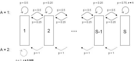
In this MDP, also sometimes referred to as a “chain MDP”, S states are arranged linearly from left to right, with state 1 on the left and stateS on the right. Initially, the system starts in state 1. There are two actions 1 and 2, with action 2 always going left, and action 1 possibly going right. There is a large reward at state S that can be obtained playing action 2 and a small reward at state 1 upon playing action 1. See Figure 2.1 for a schematic of the MDP with the specific transition and reward values that will be used in our computational study. The idea is that, optimally, action 2 should always be played because the reward in state S is large compared to the reward in state1. However, it takes some time of zero reward to get to stateS, while playing

(40)

Figure 2.1: Chain MDP withSstates and two actions. “stuck” incurring the small reward forever.

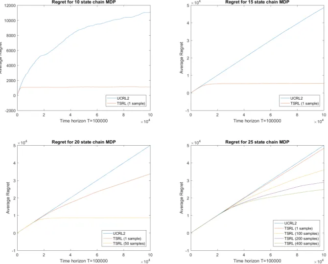
We ran 10 to 25 iterations of UCRL2 and our Thompson sampling algorithm (TSRL) with varying number of samples over a time horizon of100000on the chain MDP model with different number of states. In particular, we ran 1-sample TSRL atS = 10; 1-sample TSRL atS = 15; 1-and 50-sample TSRL atS = 20; and 1-, 100-, 200-, 400-sample TSRL atS = 25. Below in Figure 2.2 we plot the average cumulative regret over time.

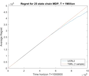
First, we notice that for this type of MDP, we outperform UCRL2 quite significantly even when there are fewer states. We also notice that increasing samples improves learning rate. However, this may not always be the case. Below in Figure 2.3 we display the average cumulative regret of 1-sample TSRL versus UCRL2 whenS = 20over a much longer time horizon of one million time steps. In fact, 1-sample TSRL appears to never learns the optimal policy, while UCRL2 shows promising signs of learning eventually. We believe this particular example is a case where multiple samples may be necessary to ensure high probability convergence to the optimal policy.

2.7 Conclusions

We presented an algorithm inspired by posterior sampling that achieves near-optimal worst-case regret bounds for the reinforcement learning problem with communicating MDPs in a

(41)

non-Figure 2.2: Average cumulative regret for chain MDPs withS= 10,15,20,25andT = 100,000. episodic, undiscounted average reward setting. Our algorithm may be viewed as a randomized version of the UCRL2 algorithm of [13], with randomization via posterior sampling. Our analysis demonstrates that posterior sampling provides the right amount of uncertainty in the samples, so that an optimistic policy can be obtained without excess over-estimation.

While our work surmounts some important technical difficulties in obtaining worst-case regret bounds for posterior sampling based algorithms for communicating MDPs, the provided bound matches the previous best bound inSandA. Obtaining a better worst-case regret bound n remains an open question. In particular, we believe that studying value functions may improve the depen-dence onS in the regret bound, possibly for largeT ([20] produce an O˜(√HSAT)bound when

(42)

Figure 2.3: Very long horizonT = 1,000,000we can see that UCRL2 begins to learn while TSRL with 1 samples still does not.

samples required in every epoch from O˜(S) to constant or logarithmic in S, and extensions to contextual and continuous state MDPs.

(43)

Algorithm 1A posterior sampling based algorithm for the reinforcement learning problem Inputs: State space S, Action space A, starting state s1, reward function r, time horizon T,

parametersρ∈(0,1].

Initialize: Setψ := 2_CSlog(SA_ρ ), η :=

q

T S

A + 12ωS

4_{, ω} _{:= 720 log(}_{T /ρ}₎_{, κ} _{:= 120 log(}_{T /ρ}₎_,

τ1 := 1.

for allepochsk= 1,2, . . . ,do

Sample transition probability vectors: For eachs, a, generateψ independent sample proba-bility vectorsQj,k

s,a, j = 1, . . . , ψ, as follows:

• (Posterior sampling): Fors, asuch thatNτk

s,a ≥η, sample from the Dirichlet

distribu-tion:

Qj,k_s,a∼Dirichlet(Mτk

s,a),

withMτk

s,a(i), i∈ Sas defined in (2.3).

• (Simple optimistic sampling): Fors, a such that Nτk

s,a < η, use the following simple

optimistic sampling: let

P_s,a− := ˆPs,a−∆,

where Pˆs,a(i) := Ns,aτk(i)

Ns,aτk , and ∆i := min

r 4 ˆPs,a(i) log(2ST) Ns,aτk + 3 log(2ST) Ns,aτk , ˆ Ps,a(i) , and letzbe a random vector picked uniformly at random from{11, . . . ,1S}; set

Qj,k s,a =Ps,a− + (1− PS i=1P − s,a(i))z.

Compute policyπ˜k:as the optimal gain policy for extended MDPM˜k_{constructed using}

sam-ple set{Qj,k

s,a, j = 1, . . . , ψ, s∈ S, a∈ A}.

Execute policyπ˜k_:

for alltime stepst=τk, τk+ 1, . . . ,untilbreak epochdo

Play actionat= ˜πk(st).

Observe the transition to the next statest+1.

SetNt+1

s,a (i), Ms,at+1(i)for alla∈ A, s, i∈ S as defined (refer to Equation (2.3)).

IfN_st_t+1_,a_t ≥2Nτk

st,at, then setτk+1 =t+ 1andbreak epoch.

end for end for

(44)

Chapter 3: MDPs with convex cost functions: Inventory Management and

Stochastic Queueing

Many operations management problems involve making decisions sequentially over time, where the outcome of a decision may depend on the current state of the system in addition to an uncer-tain demand or customer arrival process. This includes several online decision making problems in revenue and supply chain management. There, the sales revenue and supply costs incurred as a result of pricing and ordering decisions may depend on the current level of inventory in stock, back orders, outstanding orders etc., in addition to the uncertain demand and/or supply for the products. A Markov Decision Process (MDP) is a useful framework for modeling these sequential decision making problems. In a typical formulation, the state of the MDP captures the current position of inventory. The reward (observed sales) depends on the current state of the inventory in addition to the demand. The stochastic state transition and reward generation models capture the uncertainty in demand. However, unlike the setting considered in the previous chapter, the state space and action space are large and continuous.

In this chapter, we consider a more general reinforcement learning problem that relax our as-sumption that the state and action space is finit and allow continuous state and action space. In general, such RL problems are very difficult to solve; we focus on classes of RL problems that exhibit certain structure. Specifically, we consider settings where the long run cost function is convex in the decision parameters. We find that this property arises in several important operations management problems, such as inventory management and stochastic queueing. We propose an al-gorithm inspired by stochastic convex bandit optimization and first show that this alal-gorithm, when applied to inventory management, achieved efficient regret bounds. We also provide some prelim-inary examples of how this algorithm can be generalized to other applications such as stochastic

(45)

queueing, which also exhibits this convexity property. This chapter is based on joint work with Shipra Agrawal.

Organization. The rest of this chapter is organized as follows. In the next section, we give an overview of the problem setting and introduce the inventory management and stochastic queueing applications. In Section 3.2, we provide a formal problem definition and describe our main results for the inventory management problem. In Section 3.3, we use an MRP (Markov Reward Process) formulation to prove some key technical results, including convexity and bounded bias of base-stock policies. These insights form the basis of algorithm design and regret analysis in Sections 3.4 and 3.5, respectively. In Section 3.6 we give a formal problem definition to stochastic queueing application, where the long run cost is convex. Finally, we provide a comparison to relatied work in Section 3.7 and conclude in Section 3.8.

3.1 Introduction

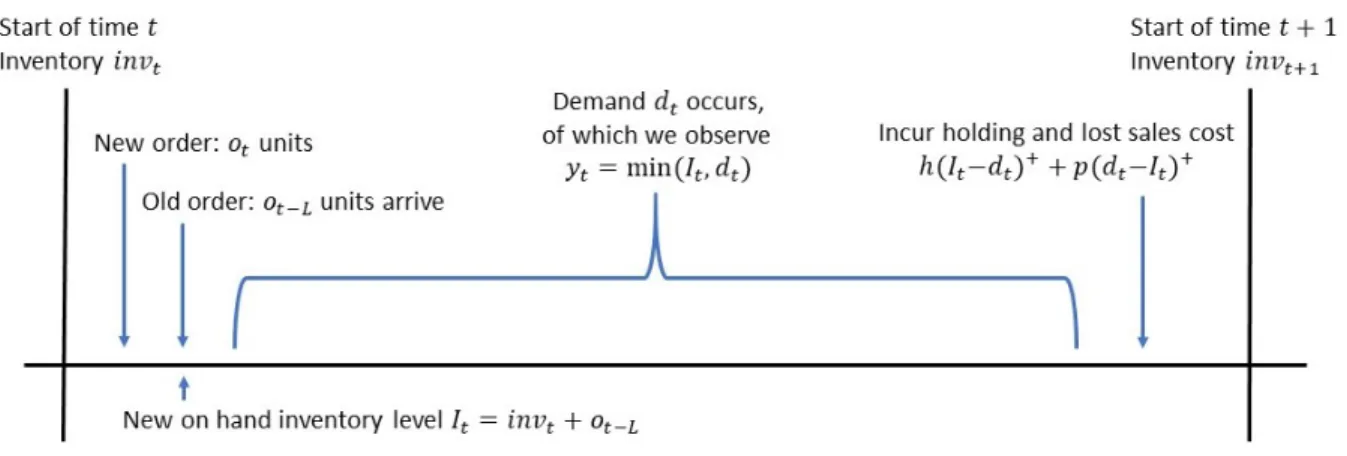
A fundamental yet notoriously difficult problem in inventory management is the periodic in-ventory control problem underpositive lead timesandlost sales[33, 34]. In this problem, in each of the T sequential decision making periods, the decision maker takes into account the current on-hand inventory and the pipeline of outstanding orders to decide the new order. There is a fixed delay (i.e., lead time) between placing an order and receiving it. A random demand is generated from a static distribution, independently in every period. However, the demand information is cen-sored in the sense that the decision maker observes only the sales, i.e., minimum of the demand and the on-hand inventory. Any unmet demand is lost, and incurs a penalty called the lost sales penalty. Any leftover inventory at the end of a period incurs a holding cost. The aim is to mini-mize the aggregate long term inventory holding cost and lost sales penalty. There is a significant existing research that develops a Markov model (or semi-Markov model as the lost sales penalty is unobserved) for this problem, and studies methods for computing optimal policies, assuming the demand distribution is either known or can be efficiently simulated(e.g., see survey in [35]).

(46)

(asymptotically with increase in lost sales penalty) for this problem [36, 35]. Under a base-stock policy, the inventory position is always maintained at a target “base-stock” level. Notably, when using a base-stock policy, the infinite horizon average cost function for the inventory control MDP can be shown to be convex in the base-stock level [37]. Therefore, under known demand model, convex optimization can be used to compute the optimal base-stock policy.

We considered a relatively less studied problem of periodic inventory control when the decision makerdoes not know the demand distribution a priori. The goal is to design a learning algorithm that can use the observed outcomes of past decisions to implicitly learn the unknown underlying MDP model and adaptively improve the decision making strategy over time, aka a reinforcement learning algorithm. Following the near-optimality of stock policies, we use the best base-stock policy as a benchmark, and aim to bound the regret of the learning algorithm compared to such a policy.

The two main challenges in designing an efficient learning algorithm for the inventory control problem described above are presented by the censored demand and the positive lead time. The censored demand assumption results in an exploration-exploitation tradeoff for the learning algo-rithm. Since the decision maker can only observe the sales, which is minimum of the demand and the on-hand inventory for a product, the quality of samples available for demand estimation of a product depend crucially on the past ordering decisions. For example, suppose that due to the past ordering policies, a certain product was maintained at a low inventory level for most of the past sales periods. Then, the higher quantiles of the demand distribution for that product would be unobserved. Therefore, in order to ensure accurate demand learning, large inventory states need to be sufficiently explored. However, this exploration needs to be limited due to the holding cost incurred for any leftover inventory. The previous chapter, and other recent work on exploration-exploitation, discusses algorithms for regret minimization in finite state, finite action MDPs, with regret bounds that depend linearly or sublinearly on the size of the state space and the action space (e.g., [13, 14, 11]). However, the positive lead time in delivery of an order results in a much en-larged state space (exponential in lead time) for the inventory control problem considered here,

New Algorithms and Analysis Techniques for Reinforcement Learning

Abstract

Table of Contents

List of Figures

Acknowledgements

Dedication

Chapter 1: Introduction

Chapter 2: Thompson sampling for Communicating MDPs

Chapter 3: MDPs with convex cost functions: Inventory Management and

Stochastic Queueing