A Dissertation by
GANGGANG XU
Submitted to the Office of Graduate Studies of Texas A&M University
in partial fulfillment of the requirements for the degree of DOCTOR OF PHILOSOPHY
December 2011
A Dissertation by
GANGGANG XU
Submitted to the Office of Graduate Studies of Texas A&M University
in partial fulfillment of the requirements for the degree of DOCTOR OF PHILOSOPHY
Approved by:
Co-Chairs of Committee, Suojin Wang Jianhua Huang Committee Members, Raymond J. Carroll
Jianxin Zhou Head of Department, Simon J. Sheather
December 2011 Major Subject: Statistics
ABSTRACT
Variable Selection and Function Estimation Using Penalized Methods. (December 2011) Ganggang Xu, B.S., Zhejiang University;
M.S., Texas A&M University
Co–Chairs of Advisory Committee: Dr. Suojin Wang Dr. Jianhua Huang
Penalized methods are becoming more and more popular in statistical research. This dissertation research covers two major aspects of applications of penalized meth-ods: variable selection and nonparametric function estimation. The following two paragraphs give brief introductions to each of the two topics.
Infinite variance autoregressive models are important for modeling heavy-tailed time series. We use a penalty method to conduct model selection for autoregressive models with innovations in the domain of attraction of a stable law indexed by α ∈ (0,2). We show that by combining the least absolute deviation loss function and the adaptive lasso penalty, we can consistently identify the true model. At the same time, the resulting coefficient estimator converges at a rate of n−1/α. The proposed approach gives a unified variable selection procedure for both the finite and infinite variance autoregressive models.
While automatic smoothing parameter selection for nonparametric function es-timation has been extensively researched for independent data, it is much less so for clustered and longitudinal data. Although leave-subject-out cross-validation (CV) has been widely used, its theoretical property is unknown and its minimization is computationally expensive, especially when there are multiple smoothing parameters. By focusing on penalized modeling methods, we show that leave-subject-out CV is
optimal in that its minimization is asymptotically equivalent to the minimization of the true loss function. We develop an efficient Newton-type algorithm to compute the smoothing parameters that minimize the CV criterion. Furthermore, we derive one simplification of the leave-subject-out CV, which leads to a more efficient algo-rithm for selecting the smoothing parameters. We show that the simplified version of CV criteria is asymptotically equivalent to the unsimplified one and thus enjoys the same optimality property. This CV criterion also provides a completely data driven approach to select working covariance structure using generalized estimating equations in longitudinal data analysis. Our results are applicable to additive, linear varying-coefficient, nonlinear models with data from exponential families.
ACKNOWLEDGMENTS
First of all, I would like to thank all my committee members: Dr. Suojing Wang, Dr. Jianhua Huang, Dr. Jianxin Zhou and Dr. Raymond J. Carroll. I am very fortunate to have them to guide my work in Texas A&M University.
Special thanks go to Dr.Wang and Dr.Huang, who are my Ph.D. dissertation advisors. During my past five years in Texas A&M University, they have given me numerous helpful advices in my research and daily life. Dr. Wang is a world class researcher in nonparametric statistics, a great teacher and a close friend of mine. Being a graduate student in a foreign country can be extremely difficult with tons of issues other than school work to deal with. Whenever I need help, Dr. Wang was always there and was always supportive for all decisions I made. He would even help fix my old car when it broke down. I respect him for his enthusiasm for work, his attitude to life, his vision of the future and his generosity to his students. I want to thank him for everything he did for me.
Dr. Huang is a very energetic and productive professor who is well known for his work in nonparametric statistics and functional data analysis. He is the one who showed me the door to research in statistics. I was always impressed by his broad and deep knowledge of all areas of statistics and his dedication to first class collaborative research with researchers from outside the Department. He guided me into many exciting areas of statistics and created the best possible research environment for me. I am very grateful to him for all his invaluable help during my years at Texas A&M University.
Dr. Carroll is a world leading statistician and a great teacher. It is a honor to have him on my committee. His insights in research helped me improve my work and made the results more profound than I originally thought. Dr. Zhou is an expert in
numerical computation and optimization. I want to thank him for his input in the computational aspect of the algorithm, which made the algorithm more efficient and stable.
I also want to thank Dr. Michael Longnecker, who is such a great teacher and a good friend. When I was working as a graduate teaching assistant, he has been constantly helpful by giving me useful advice on teaching, encouraging me when I was frustrated and backing me up in front of my classes. He is the reason I fell in love with becoming a good teacher. As the Associate Department Head, he is extremely responsible and efficient, providing timely help to all students and faculty members. I feel very lucky to have him around in my journey to my Ph.D. in Statistics.
I want to thank all my friends and colleagues in the Department. You have made my life in College Station so colorful and exciting. Finally I would like to thank my family, especially my parents. Your support has been essential.
TABLE OF CONTENTS
CHAPTER Page
I INTRODUCTION. . . 1
1.1. Variable selection using penalized methods . . . 1
1.2. Nonparametric function estimation using longitudinal data 3 II LITERATURE REVIEW FOR CHAPTER III . . . 7
2.1. Stable distribution: modeling heavy tailed distribution . . 7
2.2. Test for infinite variance: the Hill estimator . . . 11
2.3. Estimation of infinite variance autoregressive model . . . . 14
2.3.1. Least square and least absolute deviation estimator 16 2.3.2. Self-weighted least absolute deviation estimator . . 18
2.4. Order determination . . . 19
2.5. Variable selection using penalized methods . . . 21
2.5.1. Variable selection of linear regression model . . . 21
2.5.2. Variable selection of autoregressive model . . . 24
2.6. Autoregressive approximation for a stationary process . . 25
2.6.1. Weakly stationary process . . . 26
2.6.2.p-stationary process . . . 27
III VARIABLE SELECTION FOR INFINITE VARIANCE AU-TOREGRESSIVE MODELS . . . 29
3.1. Introduction . . . 29
3.2. Adaptive lasso for infinite variance autoregressive models . 31 3.2.1. Notations and Preliminaries . . . 31
3.2.2. Adaptive lasso with self-weighted least absolute deviation . . . 32
3.2.3. Adaptive lasso with least absolute deviation . . . . 36
3.2.4. Comparison with self-weighted least absolute de-viation method . . . 39
3.2.5.p-Stationary process . . . 40
3.3. A simulation study . . . 41
3.3.1. Computational formulation . . . 41
3.3.2. Tuning parameter selection . . . 42
3.4. A real data example . . . 55
IV NONPARAMETRIC FUNCTION ESTIMATION USING LON-GITUDINAL DATA . . . 57
4.1. Introduction . . . 57
4.2. Leave-subject-out cross validation . . . 61
4.2.1. Heuristic justification . . . 61
4.2.2. Loss function . . . 61
4.2.3. Regularity conditions . . . 62
4.2.4. Optimality of leave-subject-out CV . . . 64
4.2.5. Selection of working covariance structure . . . 66
4.3. Efficient computation . . . 67 4.3.1. Shortcut formula . . . 67 4.3.2. An approximation of leave-subject-out CV . . . 68 4.3.3. Algorithm . . . 68 4.4. Simulation studies . . . 72 4.4.1. Function estimation . . . 72 4.4.2. Comparison with GCV . . . 73
4.4.3. Covariance structure selection . . . 75
4.5. A real data example . . . 76
REFERENCES . . . 83
APPENDIX A . . . 91
APPENDIX B . . . 96
LIST OF TABLES
TABLE Page
1 Simulation results with Cauchy errors using SLAD-alasso with
ρ= 90% . . . 46
2 Simulation results with Cauchy errors using SLAD-alasso with ρ= 95% . . . 47
3 Simulation results with Cauchy errors using LAD-alasso . . . 48
4 Simulation results withS(1.5,0; 1) errors using SLAD-alasso with ρ= 90% . . . 49
5 Simulation results withS(1.5,0; 1) errors using SLAD-alasso with ρ= 95% . . . 50
6 Simulation results with S(1.5,0; 1) errors using LAD-alasso. . . 51
7 Simulation results with N(0,1) errors using SLAD-alasso with ρ= 90% 52 8 Simulation results with N(0,1) errors using SLAD-alasso with ρ= 95% 53 9 Simulation results with N(0,1) errors using LAD-alasso . . . 54
10 The final model for the Hang Seng Index data . . . 56
11 Simulation results for working covariance structure selection. . . 76
12 Simulation results for working covariance structure selection. . . 77
LIST OF FIGURES
FIGURE Page
1 Hill estimators of the left-handed tail index HL,k (dashed line)
and right-handed tail indexHR,k (solid line) usingiid sample . . . . 13 2 Hill estimators of the left-handed tail index HL,k (dashed line)
and right-handed tail indexHR,k (solid line) using AR(1) sample
(above) and estimated residuals (below) . . . 15 3 Original HSI dataxt (above) and the transformed data yt(below). . . 55 4 Simulation results for function estimation. Top panels: bias of
estimated functions. Bottom panels: variance of estimated func-tions. In all panels, solid curves correspond to W1, and dashed
curvesW2. . . 74
5 Relative efficiency of LsoCV* to GCV and the true loss using
working independence. . . 75 6 Width of the 95% pointwise bootstrap confidence intervals based
on 1000 bootstrap samples, using the working independence (solid
line) and the covariance matrixW2 (dashed line). . . 81
7 Fitted varying coefficient model of the CD4 data using the working covariance matrixW2. Solid curves are fitted coefficient functions;
CHAPTER I
INTRODUCTION
1.1. Variable selection using penalized methods
Heavy-tailed time series data is often encountered in a variety of fields, such as hy-drology (Castillo, 1988), economics and finance (Koedijk et al., 1990) and teletraffic engineering (Duffy et al., 1994). In this situation, the infinite variance autoregressive model is often preferred to the finite variance one, and its statistical theory has been widely studied in the literature. See Resnick (1997) for a comprehensive review and further references.
Model selection is an important aspect of modeling with time series data. An unnecessarily complex model can degrade the efficiency of the resulting parameter estimators and lead to less accurate predictions. For a time series model with finite variance, traditional model selection criteria aic (Akaike, 1973) and bic (Schwarz, 1978) can be employed to choose the order of the autoregressive model (McQuarrie and Tsai, 1998). Compared to the case of finite variance autoregressive models, few papers have investigated the model selection for autoregressive models with infinite variance. Bhansali (1988) considered the order determination of the infinite variance autoregressive processes with innovations in the domain of attraction of a stable law, and gave a consistent estimator of the order. Knight (1989) studied the same model and showed that the order selection withaicis weakly consistent. While most of the literature focuses on the order determination of the time series, Ling (2005) proposed a self-weighted least absolute deviation estimator for the infinite variance autoregressive model under which the coefficient estimates are asymptotically normal
and thus can be used for statistical inference. He also proposed a variable selection procedure with a series of hypothesis tests based on the self-weighted least absolute deviation estimator. However, his method can be unstable and its implementation is complicated.
Using the shrinkage method for variable selection is relatively new in time series literature. Wang et al. (2007a) applied adaptive lasso (Zou, 2006) to the regression model with finite autoregressive errors. They showed that the resulting estimator via adaptive lasso not only has a sparse presentation, but also has the oracle property (Fan and Li, 2001), which means that it can simultaneously select variables and estimate parameters in time series modeling.
One difficulty often encountered in data analysis is that it is generally impossible to know whether a time series of finite length has infinite variance (Granger and Orr, 1972). Many methods have been developed to test for infinite variance of a real time series data; see, for example, Hill (1975). While Wang et al. (2007a)’s method does not apply to infinite variance autoregressive models, using Ling (2005)’s method can cause loss of important information by weighing down large observations, especially in the case of a time series with heavy tails but finite variance.
In Chapter III, we first use the self-weighted least absolute deviation proposed by Ling (2005) as the loss function and the adaptive lasso as the penalty method to do the model selection. Under appropriate conditions, we show that our penalized method can identify the true model consistently and the estimator of the coefficients corresponding to the true model is asymptotically normal, which is important for the statistical inference of infinite variance autoregressive models. After that, we propose a unified variable selection approach that can efficiently deal with heavy-tailed autoregressive models with either finite or infinite variance. By combining the least absolute deviation as the loss function and the adaptive lasso as the penalty
function, we show that under regularity conditions we can identify the true model consistently and obtain a point estimator of the coefficients corresponding to the true model with a convergence rate of n−1/α, where α ∈ (0,2) is the index of the stable distribution. This convergence rate is faster than that of finite variance time series.
1.2. Nonparametric function estimation using longitudinal data
Longitudinal data analysis has been a subject of intense research in statistics for the past 30 years. Various parametric models (e.g. Vonesh and Chinchilli, 1997; Diggle et al., 2002) and nonparametric or semi-parametric models (e.g. Hart and Wehrly, 1986; Rice and Silverman, 1991; Zeger and Diggle, 1994; Fan and Zhang, 2000; Lin and Carroll, 2000; Wang et al., 2005) have been proposed and studied. In a typical set of longitudinal data, we have observations (yij,xij), forj = 1, . . . , ni,i= 1, . . . , n, where yij is the response variable of jth measurement of the ith subject and the
xij is the corresponding p×1 vector of covariates. It is reasonable to assume that observations from different subjects are independent and observations within a subject are correlated. For the longitudinal data analysis, there are three main modeling families: marginal models, mixed-effect models, and transition models (Diggle et al., 2002). In Chapter IV, we focus on the marginal approach using generalized estimating equations (GEE, Liang and Zeger, 1986).
By introducing a parameterized working correlation, GEE method has the poten-tial to increase the efficiency of the regression estimates when the marginal distribu-tion of response are from exponential family. More specifically,yij is from exponential family with meanµij and variance vij,
f(yij) = exp
yijθij −b(θij)
φ +c(yij, φ)
where µij =b′(θij),vij =φb′′(θij) and with the link functiong(µij) =xT ijβ.
One limitation of the work of Liang and Zeger (1986) is its inflexibility because it assumes fully parametric relationship between the response and covariates. Non-parametric and semi-Non-parametric models are developed to model more complicated relationships in the longitudinal data setup. These work include generalized additive models (GAM, Wild and Yee, 1996; Berhane and Tibshirani, 1998; Lin and Zhang, 1999), varying coefficient models (Hoover et al., 1998; Chiang et al., 2001; Huang et al., 2002), partially linear models (Zeger and Diggle, 1994; He et al., 2002; Wang et al., 2005; Huang et al., 2007), and partial linear varying coefficient model (Ahmad et al., 2005). All above mentioned models can be viewed as special cases with link function defined as:
g(µij) = xij0β0+
m
X
k=1
fk(xijk),
where xij0β0 is the strictly parametric part of the model and fk, (k = 1, . . . , m) are
unknown smooth functions (xijk can either be a scaler or a vector).
The flexibility of the GAM is also accompanied by the potential risk of over-fitting the data. Broadly speaking, the estimation of nonparametric terms in (4.2) can be classified into kernel methods (Wand and Jones, 1995) and spline methods (Green and Silverman, 1994). The kernel method avoids over-fitting by selecting appropriate bandwidth for each nonparametric component using cross validation. However, the estimation of kernel coefficient itself can be computationally challenging, the selection of bandwidths can be computationally prohibitive for generalized additive models, if not impossible. In addition, Welsh et al. (2002) pointed out that, by taking into account of the within subject correlation, the spline methods appear to be more efficient than the kernel methods in nonparametric marginal regression model. In Chapter IV, we using spline methods to estimate the nonparametric function. To
avoid over-fitting, Berhane and Tibshirani (1998) proposed to use the ”Penalized Quansi-Likelihood” criterion: P(f1,· · · , fk) = Q(η;y)− 1 2 m X k=1 λkJ(fk)
where η=g(µ), Q(η;y) is some quasi-likelihood score function based on data, J(·) is some penalty functional and λ1,· · · , λk are smoothing parameters controlling the
tradeoff between model fit and model complexity.
(Example 1: Partial linear additive model) The response Y is related to the covariates X = (X1,· · ·, Xm)T ∈Rm and Z = (Z1,· · · , Zd)T ∈Rd in the way:
µ=E(Y|X =x, Z =z) = g−1(zTβ+ m
X
k=1
fk(xk))
wherexk is thekth component ofx,β is ad-dimensional vector andfk’s are unknown and smooth functions. Then in this case, we can take Q(η;y) as the log-likelihood function of y and the penalty functional defined as J(fk) =R
[f′′(xk)]2dxk.
(Example 2: Varying coefficient model) Hoover et al. (1998) considered the model yij =XijTβ(tij) +ǫi(tij),
where β(t) = (β0(t),· · · , βm(t))T (m ≥ 0) are unknown smooth functions of t, ǫi(t)
is a realization of a zero-mean stochastic process ǫ(t), (t ∈ R), and Xij and ǫi are independent. In this case, fk(·)’s are bivariate functions except for k = 0. More specifically, for k= 0,· · ·, m, we would havefk(xk,ij) =Xk,ijβk(tij) whereXk,ij is the kth component ofXij andX0,ij = 1. Here, we take Q(η;y) =−Pi,j(yij−XijTβ(tij))2 and the penalty term as J(fk) =R
[β′′
k(t)]2dt for k= 0,· · · , m.
The choice of λk’s is critical for getting a good function estimator. If there is no intra-subject correlation and treat all observations as independent data points, the asymptotic optimality of generalized cross validation (GCV, Craven and Wahba,
1979) in selecting smoothing parameters has been showed by Li (1986) in ridge regres-sion and by Gu and Ma (2005) in the case of mix effect model. However, when there is intra-subject correlation as in longitudinal or cluster data, smoothing parameters selection is still an open problem. One of the popular procedure in this area is called “leave-subject-out cross-validation” (LsoCV), see Rice and Silverman (1991); Hoover et al. (1998); Huang et al. (2002). As popular as it is, there are several issues with this procedure. First of all, the computational cost of doing cross-validation is expensive. Furthermore, in the current practice in longitudinal study, researchers still rely on the grid search to find the optimal λ’s using leave one subject out cross-validation. Because of this, current research can only deal with one or two smoothing parame-ters, searching in a higher dimension is not feasible. This is especially not desirable in varying coefficient model where each nonparametric component is supposed to receive different amount of penalty. The other issue with the LsoCV method is that even though it is widely used, no theoretical properties nor a systematic algorithm for it have yet been developed.
In Chapter IV, we first derive a short cut formulae for the LsoCV score and show that it is asymptotically optimal in selecting smoothing parameters in the sense that under certain conditions, minimizing LsoCV score is equivalent to minimizing the MSE of the function estimator when number of subjects goes to infinity. We then propose a new computationally more efficient criterion for choosing optimal smoothing parameters while maintain the asymptotical optimality. Based on the new criterion, a Newton-Raphson type algorithm is developed for automatically selecting multiple smoothing parameters. In the end, a completely data driven approach of selecting the best working covariance structure is proposed based on the LsoCV method.
CHAPTER II
LITERATURE REVIEW FOR CHAPTER III
2.1. Stable distribution: modeling heavy tailed distribution
Heavy-tailed time series data is often encountered in a variety of fields, such as hy-drology (Castillo, 1988), economics and finance (Koedijk et al., 1990) and teletraffic engineering (Duffy et al., 1994). But what is a heavy tail? We use the definition proposed in Resnick (1997). A random variable X is said to have a light tailed dis-tribution if it decay exponentially fast as x→ ∞,
P[|X|> x]∼ √1 2π
exp(−x2/2)
x →0.
The most famous example in this class is the Normal distribution. A random variable X is said to have a heavy tailed distribution F(x) with index α >0 if, for x >0,
P(|X|> x) =x−αK(x), (2.1) where K(x) is some slowly varying function, that is, for x >0
lim t→∞
K(tx) K(t) = 1. This definition implies that
E(|X|β)<∞, β < α, E(|X|β) = ∞, β > α. (2.2)
As mentioned in Resnick (1997), typical examples of K(x) include: K(x) = c, Pareto distribution; c+o(1), Stable distribution; log(x), x >1;
1/log(x), x >1;
The difference term o(1) between the tail behavior of the pareto distribution and the stable distribution may look negligible, but it can cause big differences in detecting two types of tails.
One thing worth mentioning is that, when the tail index of F(x) is less than 2, that is α <2, the random variableX would have infinite variance. One consequence is that when a time series or other stochastic processes have error terms of infinite variance, many of the classical methods of analysis based on second moments, for example, regression, autoregressive models and spectral analysis, may not be used properly for such series (Granger and Orr, 1972).
To model distributions with infinite variance, one of the popular choices is the stable distribution law, which can be defined in several different ways. Granger and Orr (1972) gives a detailed summary of stable distribution and we cite some of their results here.
Definition: A distribution function F(x) is called stable if for every a1 > 0, b1
and a2 >0, b2, there exists corresponding a and b such that the equation
F(a1x+b1)∗F(a2x+b2) = F(ax+b)
holds, where ∗ denotes the convolution operator.
indepen-dent random variables having the same stable distribution function F(·), then the sum X+Y also has the same stable distribution function F(·). This additive defini-tion of stable distribudefini-tion results in a generalized version of central limit theorem as the following (Granger and Orr, 1972).
Generalized Central Limit Theorem Let{Xn} be a sequence of iid random vari-ables and {an} and {bn} be two sequence of numbers, define the sums
Sn = 1 an n X i=1 Xi−bn.
If weighted sum sequence Sn converges in distribution as n → ∞, then it must converge to a random variable with a stable distribution.
This theorem provides a heuristic justification for the use of stable distribution to model the error terms in time series. For example, if a variable in an economic time series can be considered as sums of a large number of independent terms (like the stock price, which can be viewed as a consequence of numerous independent transactions), the distribution of the series might have infinite variance, when the infinite invariance stable distribution may be a reasonable tool to model this types of data.
A necessary and sufficient condition for the distribution functionF(·) to be stable is that its characteristic function φ(t) admits the following representation:
φ(t) = exp{iγt−δ|t|α[1 +iβsgn(t)w(t, α)]},
where i=√−1, 0< α ≤ 2, −1≤ β ≤1, δ ≥ 0, γ is any real number and functions w(t, α) and sgn(·) are defined as
w(t, α) = tanπα2 , α 6= 1; 2 π log|t|, α= 1; , sgn(t) = 1, t >0; 0, t= 0; −1, t < 0.
This characterization completely describes all members of stable distribution family. Unfortunately, for most values of parameters α, β, γ and δ, F(·) does not have a analytical form. Two special cases are, if α = 2, F(·) is the cumulative distribution function of Normal distribution and α = 1, β = 0 case corresponds to the Cauchy distribution.
Definition For a sequence ofiidrandom variables{Xn}with distribution function F(·), F(·) is said to belong to the domain of attraction of a stable distribution if for some sequence of numbers {an} and {bn},
Sn= 1 an n X i=1 Xi−bn→F(·) in distribution, as n→ ∞.
A sufficient and necessary condition for the distribution function F(·) to be in the domain of attraction of the stable law with index α ∈(0,2) is that
lim x→∞ P(X1 > x) P(|X|> x) ≡q∈[0,1] exists and P(|X1|> x) = x−αK(x),
where K(x) is a slowly varying function defined in equation (2.1). This condition together with equation (2.2) implies that distribution functions belong to the domain of attraction of the stable law have heavy tails. Furthermore, sinceα ∈(0,2], except the Normal case (α = 2), all members of stable distributions have infinite variance and even infinite first moment for thoseα <1.
In Chapter III, we shall use the assumption that the innovations of the autore-gressive models with infinite variance belong to the domain of attraction of the stable law with index α∈(0,2].
2.2. Test for infinite variance: the Hill estimator
As stated in Granger and Orr (1972), having observed a series {y1,· · · , yn} with a
finite length, it is usually impossible to distinguish whether it has infinite variance or not. Among many others, one important reason why identifying heavy tail distri-bution is necessary is due to the efficiency of estimation. For a parametric model, the most efficient estimator for parameters in the model is the maximum likelihood estimate. Misspecification of distributions of the observations would lead to loss in efficiency of estimators. For example, it is shown in Davis et al. (1992) that, for au-toregressive models with innovations belong to the domain of attraction of the stable law with index α ∈ [1,2), the least absolute deviation (LAD) estimator is asymp-totically much more efficient than the least square (LS) estimator. However, if the innovations are from Gaussian process, then the LS estimator is the most efficient estimator that outperforms the LAD estimator. So in this sense, it is important to identify whether the heavy tail exists in a observed process in order to choose most efficient estimation tools.
Many numerical and graphical testing procedures have been proposed for testing the existence of heavy tail distributions. One of the widely used procedure is the Hill estimator (Hill, 1975). Suppose X1,· · · , Xn are iid from a distribution F(·). The
left-hand and right-hand Hill index are defined as: HL,k = ( 1 k k X i=1 log X(i) X(k+1) )−1 , HR,k = ( 1 k k X i=1 log X(n−i+1) X(n−k) )−1 (2.3) where X(1) < X(2) < · · · < X(n) are order statistics and k < n. It has been shown
that if {Xn}is a stationary M A(∞) process and the marginal distribution satisfies P(|X1|> x) =x−αK(x),as x→ ∞,
then if k/n→0 as k→ ∞ and n → ∞, we have
HL,k −→p α,and HR,k −→p α,
where the notation−→p stands for converge in probability. More details about the Hill estimator can be found in, for example, Resnick (1997). Applying to our setting of stable distribution, this result asserts that the Hill estimator is an consistent estimator of the indexαif the marginal distribution of a process is from the domain of attraction of the stable law. If the estimated ˆα <2, then we will have strong evidence to believe that this process has an infinite variance.
We are interested in the autoregressive model with innovation having infinite variance, Resnick (1997) proposed following two ways to estimate α. Suppose now we have observationsy1,· · ·, yn from an autoregressive model
yt=φ1yt−1+· · ·+φpyt−p +ǫt,
whereP(|ǫ1|> x) =x−αK(x). Then
1. we can apply the Hill estimator defined in (2.3) directly to observedy1,· · · , yn.
The reason is that, by a result of Cline (1983), one has P(|y1|> x)∼(const)P(|ǫ1|> x),
which implies that the tail of y1 contains the same information as the tail ofǫ1.
2. Find consistent estimates for parameters φ1,· · · , φp first and then apply the
Hill estimator to the estimated residuals as in (2.3).
Based on the existing empirical results in literature, the second one is usually consid-ered to be a better procedure.
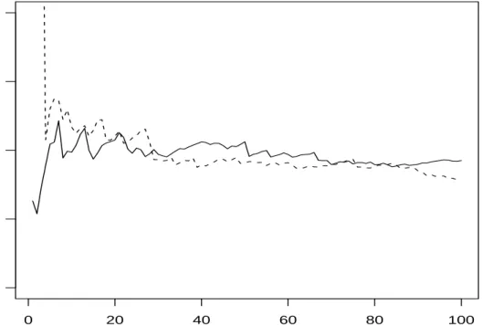
in practice, the Hill estimator is used by plotting graphs{(k, HL,k),1≤ k ≤ n} and {(k, HR,k),1 ≤ k ≤ n}, hoping both graphs look stable so that we can pick out a value of α. These graphs are useful even when a good value of α cannot be observed but a rough range of α is observable from these graphs, which is sufficient for us to determine whether the distribution has a heavy tail.
0 20 40 60 80 100 0.0 0.5 1.0 1.5 2.0 k Hill estimator
Figure 1. Hill estimators of the left-handed tail index HL,k (dashed line) and right-handed tail indexHR,k (solid line) using iid sample
To illustrate the use of the Hill estimator, we simulate n = 400 independent random numbers from standard Cauchy distribution (α= 1, β= 0). Figure 1 graphs {(k, HL,k) : 1 ≤k≤100}and{(k, HR,k) : 1 ≤k ≤100}, where we can clearly see that both curves stabilize around true value α = 1 when k increases. From Figure 1, we
can easily conclude that this distribution has a very heavy tail. To further illustrate the application of the Hill estimator to the autoregressive model, we simulate the process y1,· · · , y400 from the model
yt= 0.5yt−1+ǫt,
where ǫt is generated independently from standard cauchy distribution. Figure 2 graphs {(k, HL,k) : 1 ≤ k ≤ 100} and {(k, HR,k) : 1 ≤ k ≤ 100} using the observed datay1,· · · , y400and the estimated residuals by plugging in the least square estimator
of φ whose true value is 0.5, repectively. As proposed in Resnick (1997), applying the Hill estimator to the estimated residuals appears to be much better in turns of producing a stable value of α in the graph. However, the Hill estimator applying to the observed AR(1) process also provides sufficient evidence to reveal the heavy tailed nature of the innovation process{ǫt}.
2.3. Estimation of infinite variance autoregressive model
Consider a stationary autoregressive time series{yt} which is generated by
yt=φ1yt−1+· · ·+φpyt−p +ǫt, (2.4) where φ = (φ1, . . . , φp)T is an unknown parameter vector with its true value φ0 =
(φ0
1, . . . , φ0p)T and {ǫt} is a sequence of independent and identically distributed errors whose common distribution belongs to the domain of attraction of a stable distribu-tion with index 0< α <2. In other words,
0 20 40 60 80 100 0.0 1.0 2.0 k Hill estimator 0 20 40 60 80 100 0.0 1.0 2.0 k Hill estimator
Figure 2. Hill estimators of the left-handed tail index HL,k (dashed line) and right-handed tail index HR,k (solid line) using AR(1) sample (above) and estimated residuals (below)
whereK(x) is a slowly varying function at ∞and lim
x→∞P(ǫt > x)/p(|ǫt|> x) =q, 0≤q≤1. (2.6) This assumption on the innovation process is wildly used in the literatures (Knight, 1989; Davis et al., 1992) and it appears that many financial data series are heavy tailed in this sense. Notice that ifK(x) is a constant, then the corresponding distribution is a Pareto-like distribution, which contains the Cauchy distribution and general stable distributions as its special cases.
Furthermore, we assume that the characteristic polynomialφ(z) = 1−φ0
1z−· · ·−
φ0
pzp of model (2.4) has all roots outside the unit circle, which makes {yt} strictly stationary and ergodic. Thus we can represent the infinite variance autoregressive model (2.4) as a linear process
yt= ∞ X j=0 ψj0ǫt−j, (2.7) whereψ0
j’s are the coefficients of zj in the power series expansion of 1/φ(z).
2.3.1. Least square and least absolute deviation estimator
The least square (LS) estimator ˆφLS of φis defined as the minimizer of VLS(φ) =
n
X
t=p+1
(yt−φ1yt−1+· · ·+φpyt−p)2, (2.8)
and the least absolute deviation (LAD) estimator ˆφLAD is obtained by minimizing VLAD(φ) =
n
X
t=p+1
|yt−φ1yt−1+· · ·+φpyt−p|. (2.9)
Although intuitively, ˆφLS and ˆφLAD may not work since under assumptions (2.5) and (2.6), the autoregressive model (2.4) has infinite variance whenα < 2, and even infinite mean when α < 1. However, both of them perform surprisingly well in practice. Davis et al. (1992) provides a heuristic explanation of this phenomenon. They argued that it is true that large positive or negative values of ǫt produce points appearing to be outliers. However, each one of theseoutliers will produce a sequence of leverage points, which would compensate for the negative effect of the outliers and lead to faster convergence rates of both ˆφLS and ˆφLAD than in the finite variance setting. Furthermore, since VLAD(φ) gives less weight to the outliers while giving similar weight to the leverage points, ˆφLADis reasonably expected to be more efficient
than ˆφLS, which is later confirmed by their theoretical results.
For the LS estimator ˆφLS, Davis and Resnick (1985) and Davis and Resnick (1986) show that, under assumptions (2.5) and (2.6), there exists a slowly varying function K0(n) such that:
n1/αK0(n)( ˆφLS −φ0)→ξ0 in distribution, as n→ ∞, (2.10)
whereξ0 is the ratio of two stable random variables. If{ǫt}is generated from a stable
distribution, then K0(n) = (logn)−1/α.
Theorem 4.1 in Davis et al. (1992) establishes the asymptotic property of ˆφLAD, which asserts that under conditions of section 2.3 together with several mild technical conditions, one has
n1/αK1(n)( ˆφLAD−φ0)→ξ in distribution, asn → ∞, (2.11)
where K1(x) is some slowly varying function such that n1/αK1(n) = bn with bn =
{infx:P(|ǫ1|> x)≤n−1} and ξ is some unknown random vector. For more details,
please refer to Davis et al. (1992).
Now compare equations (2.10) and (2.11), since for Pareto-like and stable dis-tributions, K1(x) is constant and K0(n) = (logn)−1/α (Davis et al., 1992), one can
immediately get that, as n → ∞
||φˆLAD−φ0||
||φˆLS −φ0||
p − →0,
which proves the conjecture that ˆφLAD is more efficient than ˆφLS, at least for Pareto-like and stable distributions.
2.3.2. Self-weighted least absolute deviation estimator
One of the major problem with the LS and LAD estimators is that their limiting distributions do not have closed forms. This can be seen from the fact thatξ0 and ξ
in equations (2.10) and (2.11) generally do not have closed form distributions. The immediate consequence is that we cannot perform statistical inference based on ˆφLS and ˆφLAD. To overcome this difficulty, Ling (2005) proposed a new estimation method named self-weighted least absolute deviation (SLAD) estimation for infinite variance autoregressive models, where the estimator ˆφSLAD is obtained by minimizing
VSLAD(φ) = n
X
t=p+1
wt|yt−φ1yt−1+· · ·+φpyt−p|, (2.12)
with wt as a pre-given function of {yt−1,· · · , yt−p}. By imposing some conditions on
the choice of wt and the distribution of ǫt, Ling (2005) shows that the limiting dis-tribution of ˆφSLAD is normal distribution. DenoteXt= (yt−1,· · · , yt−p)T. Following
are two additional conditions to those in section 2.3 used in Ling (2005): Condition 1: E{(wt+w2
t)(||Xt||2+||Xt||3)}<∞.
Condition 2: The error process{ǫt}has a marginal distribution with 0 median and a differentiable density f(·) such that f(0) >0 and supx∈R|f′(x)
|<∞. The choice of the weight function is the critical step to ensure the asymptotic normality of ˆφSLAD. Ling (2005) proposed to use the following weight function
wt= 1 if ct= 0, C3/c3 t, if ct6= 0, where ct =Pp
k=1|yt−k|(|yt−k| ≥C), andC can be chosen as the 90% or 95% quantile
(2005) shows that n1/2( ˆφSLAD−φ0)→N 0, 1 4f2(0)Σ−1ΓΣ−1 in distribution, as n→ ∞, where Γ =E(w2 tXtXtT) and Σ =E(wtXtXtT).
The normality of the estimator ˆφSLAD enable us to do statistical inferences such as hypothesis tests as in the finite variance case, which is a break through in the research of infinite variance autoregressive models. By conducting a series of Wald tests, one should be able to do the forward, backward or stepwise model selection. However, as in the linear regression case, these model selection methods can be un-stable and it is difficult to control the overall type I error of conducting multiple hypothesis tests. To overcome this difficulty, we propose to conduct the model selec-tion of infinite variance autoregressive model using penalized methods as will been shown later.
2.4. Order determination
Order determination is an important aspect of using an autoregressive model. Given a time series {yt}, if the true underlying structure of this process is autoregressive, what is the true value of p in model (2.4)? If the true underlying structure is not autoregressive, for example, the moving average process, what is the smallestp that will give a reasonable fit to the observed series? These problems have been studied extensively for finite variance autoregressive models, but much less for the case when the error process {ǫt} has infinite variance.
Bhansali (1988) considered the order determination for autoregressive processes under the same assumptions as in section 2.3, and gave a consistent estimator of the
orderp. Suppose we have observed a series y1,· · ·, yn, define quantities γ(k, n) = n−k X t=1 ytyt+k, and ρ(k, n) = γ(k, n)/γ(0, n),
where k = 0,±1,· · · ,±n−1. And the estimated normalized variance is given by ˆ σ2(p) = p X j=0 ˆ φjρ(j, n), p= 0,· · · , P, (2.13)
where ˆφ is some estimator of φ and P is some given integer. To obtain the optimal order ˆpopt, Bhansali (1988) proposed to choose the bestpfrom 0,· · · , P by minimizing following two criterions
F P EYα(p) = ˆσY2(p)(1 +αp/n), F P ELα(p) = ˆσ2L(p)(1 +αp/n),
where α ∈ (0,2] is the index of the stable law distribution of {ǫt} and ˆσ2
Y(p) and ˆ
σ2
L(p) are obtained by plugging Yule-Walker and least square estimates of φ into equation (2.13), respectively. Bhansali (1988) later proved that under conditions of section 2.3, minimizing either F P EYα(p) orF P EYα(p) would consistently choose the true value ofp with probability 1, asn → ∞.
Knight (1989) also studied the order determination of the autoregressive models under the same conditions as in Bhansali (1988). Knight (1989) proposed to mini-mizing the following aic type criterion
aic(p) =nlog ˆσY2(p) + 2p, p= 0,· · · , P, where ˆσ2
Y(p) is the same as in F P EYα(p). The conclusion of Knight (1989) is that, under conditions of section 2.3, if ˆp=argmin0≤p≤P aic(p), then we have
ˆ
as n → ∞, where −→p stands for convegence in probability. There have been a few of works studying the order determination of time series other than autoregressive models, for example, GARCH model with infinite variance, but our focus here is on the stationary autoregressive models with infinite variance.
2.5. Variable selection using penalized methods
2.5.1. Variable selection of linear regression model
The consistent order estimators in section 2.4 can significantly reduce the model complexity of the autoregressive model and thus lead to more efficient estimation of the model coefficients. However, even when the order of a time series is correctly identified, there is still a possibility that some of the coefficients φ0
j’s are zeros and including those zero coefficients will also result in an unnecessarily complex model which degrade the efficiency of the coefficient estimators and leads to less accurate predictions. This is especially true for long-memory autoregressive models whose order can increase as n increases. In addition, a model with a sparse representation reveals the underlying structure of the observed process. Therefore, variable selection can be a very important aspect of autoregressive models.
The idea of using penalized methods to do variable selection is pioneered by the revolutionary paper Tibshirani (1996) in the linear regression setting. Consider the linear regression model:
yi =xTi β+ǫi, i= 1,· · · , n, (2.14) whereβ is a p×1 coefficient vector andǫi’s are iid random errors with variance σ2.
To obtain the estimate of β, the Lasso method aims at minimizing Lasso(β) = n X i=1 (yi−xTi β)2+λn p X j=1 |βj|, (2.15)
whereλn>0 is a tuning parameter used to obtain a balance between model fit and model complexity. By shrinking the value ofλ towards 0, some components ofβ will be shrunk to exact 0, which means those corresponding covariates are excluded from the model. The primary advantage of theLasso method is that it can simultaneously do variable selection and model estimation, which is more stable than subsets selection in the sense that small changes in the data will not result in big change of the model selection result. Another advantage is that, as in ridge regression, the shrinkage in coefficients will help improve the prediction accuracy of the fitted model.
As appealing as the Lasso method is, Zou (2006) along with several other re-searchers pointed out that theLasso variable selection result is not consistent under certain conditions. Denote β0 = {β10,· · · , βp0} as the true value of β and S = {j : β0
j 6= 0, j = 1, . . . , p} and Snlasso = {j : ˆβjlasso 6= 0, j = 1, . . . , p} as the nonzero coefficients estimated via the Lasso method. By inconsistency, we mean that
lim n→∞P(S
lasso
n =S)<1.
In other words, under certain conditions, no matter how large your sample sizes is, there is a positive possibility that we will end up with an incorrect model using the Lasso method. To solve this problem, Zou (2006) proposed to use a modification of the Lasso method, named as the Adaptive Lasso method, which estimates β by minimizing aLasso(β) = n X i=1 (yi−xTi β)2+λn p X j=1 wj|βj|, (2.16) where w is a known weights vector. Zou (2006) suggested using wj = 1/|β˜j|γ with
γ > 0 and ˆβ being a √n-consistent estimator to β0. Again, define Snalasso = {j : ˆ
βalasso
j 6= 0, j = 1, . . . , p}as the nonzero coefficients estimated via the Adaptive Lasso method, Zou (2006) showed that if λn/√n → 0 and λnn(γ−1)/2 → ∞, then the
Adaptive Lasso estimator enjoys a so-called “Oracle property” (Fan and Li, 2001), which includes:
1. Consistency in variable selection: limn→∞P(Salasso
n =S) = 1, 2. Asymptotic normality: √n( ˆβSalasso−β0S)
d −
→N(0, σ2C−1
S ), whereCS = limn→∞ 1nXT
SXS with XS being the design matrix only using covariates with nonzero estimated coefficients. “Oracle property” means that we can simulta-neously do variable selection and model estimation as if the true model is known.
The Adaptive Lasso method is not the only penalized method that enjoys this “Oracle property”. Another famous example would be the smoothly clipped absolute deviation (SCAD) penalty function proposed in Fan and Li (2001). Zou and Li (2008) further proposed to modify the penalty term in (2.16) by replacing eachλnwj term withp′
λn(|φ˜1j|) for some general penalty function pλ(·), for example, the SCAD penalty function, which maintains the “Oracle property”.
Wang et al. (2007b) considered the model (2.14) with the error termǫifrom some heavy tailed distribution, where they proposed to do model estimation and variable selection using theLad-Lasso method by minimizing
LadLasso(β) = n X i=1 |yi−xTi β|+ p X j=1 λj|βj|, (2.17) where the tuning parameters can be chosen as
λj =λnlogn
n|βj˜|, j = 1,· · · , p,
estima-tors of β. The use of least absolute deviation loss function in (2.17) instead of the least square loss function handles the problem of having residuals from heavy tailed distributions including those with infinite variances by assigning smaller weights to large values of deviations. Assuming that the error ǫi has a continuous density func-tion f(·) such that f(0) > 0, then under certain conditions, Wang et al. (2007b) showed that as n→ ∞,
P( ˆβSc = 0)→1, and √n( ˆβS −β0S)−→d N(0, 1 4f2(0)C
−1
S ),
which implies that theLad-Lasso method also enjoys the “Oracle property”. This ac-tually motivates us to consider apply theLad-Lassomethod to model infinite variance autoregressive model.
2.5.2. Variable selection of autoregressive model
Using the shrinkage method for variable selection is relatively new in time series literature. Wang et al. (2007a) applied adaptive lasso (Zou, 2006) to the regression model with finite autoregressive errors. They considered the model
yt =xTtβ+ǫt, t = 1,· · · , n
with the error term ǫt having a finite fourth moment and following a AR(q) process ǫt=φ1ǫt−1+φ2ǫt−2+· · ·+φqǫt−q+et
where φ = (φ1,· · · , φq)T is the coefficient vector. The estimation of this model
involves the regression parameter β and the autoregressive parameter φ, which is achieved by minimizing n X t=q+1 " yt−xTtβ− q X l=1 φl(yt−l−xTt−lβ) #2 + p X j=1 λj|βj|+ q X l=1 γl|φl|,
where the tuning parameters can be chosen in the following manner λj =λnlogn
n|βj˜| and γl =γn logn n|φl˜|,
with ˜β and ˜φ being the unpenalized least square estimator or other √n−consistent estimators of β and φ. Define the index sets S1 = {1 ≤ j ≤ p : βj 6= 0} and
S2 ={1≤l≤q :φl 6= 0}, Wang et al. (2007a) showed that under certain conditions,
as n → ∞, the resulting estimators ˆβ and ˆφ have the following property P( ˆβSc
1 = 0)→1 and P( ˆφS2c = 0)→1,
which means that all those insignificant components of regression and autoregressive coefficients can be consistently excluded from the estimated model. This is an ap-pealing property that for the autoregressive part, one would not only be able to do the order determination but also variable selection. We would apply a similar idea to the infinite variance autoregressive model.
2.6. Autoregressive approximation for a stationary process
Let (Ω, FY, P) be a probability space. A zero mean stochastic process {yt}is said to be strictly stationary if the finite dimension joint cumulative distribution function of {yt} at times t1+s,· · · , tk+s satisfies
FY(yt1+s,· · · , ytk+s) =FY(yt1,· · · , ytk)
for allk ands >0. A simple example would be the white noise process with identical distribution. Following similar notations of Cheng et al. (2000), for each process {yt}
with yt∈Lp(Ω), that is, R Ω|y|
pdFY(y)<∞, we define the following subspaces: Ht(Y) = ¯sp{ys, s≤t},and H−∞(Y) = \
t≤0
Ht(Y)
where ¯sp{· · · } represents the closed linear space spanned by the elements in the bracket under the Lp norm.
The process {yt} is said to be deterministic if Ht−1(Y) =Ht(Y)
for all t, and is called nondeterministic otherwise. If a nondeterministic process satisfies
H−∞={0}, then it is said to be a pure nondeterministic process.
2.6.1. Weakly stationary process
In most situations, strict stationarity is too strong of an assumption in prediction theory of stationary process. A zero mean stochastic process {yt} is called a weakly stationary process if
E|yt|2 <∞,and cov(ys, yt) = γ(s−t), for all s, t, where γ(·) is referred to as the covariance function.
The weakly stationary process has been extensively studied and it can be shown that, any weakly stationary process with a continuous spectral density can be approx-imated by a weakly stationary autoregressive model with a large order (Brockwell and Davis, 1991). In fact, it is shown in Pourahmadi (1988) that for a purely nondeter-ministic weakly stationary process {yt}, there exists a unique series {ak} such that
for all t, one has yt= ∞ X k=1 akyt−k+ǫt, provided that P∞
k=1akyt−k is convergent in the L2 norm. A sufficient condition for
the convergence of P∞
k=1akyt−k is that
P∞
k=1|ak|<∞.
Another nice property of this decomposition is that variables in the innovation process {ǫt} are orthogonal under the inner product induced by the L2 norm, i.e.,
they are uncorrelated. This is a very useful result which indicates that, for a general weakly stationary process, we can use an autoregressive model with a sufficiently large order to do one-step or multi-step predictions, without knowing the true probability structure of the process.
2.6.2. p-stationary process
The popularity of the autoregressive model in time series studies is largely due to the fact that any second order stationary process with symmetric continuous spectral density can be approximated by an autoregressive process (Brockwell and Davis, 1991). It would be very appealing if this type of approximation still holds for the infinite variance process, which can justify the use of autoregressive model to do predictions. However, even for the strictly stationary process with infinite variance, this is difficult to show.
Miamee and Pourahmadi (1988) established such a relationship for thep-stationary process. A discrete time stochastic process{yt} is said to be ap-stationary process if
E|yt|p <∞,and E n X k=1 ckytk+h p =E n X k=1 ckytk p ,
(1< p ≤2) for all integersn≥1,t1, . . . , tn,h, and scalarsc1, . . . , cn. Note that, when
variance. This class of processes includes the harmonizable stable processes of orderα withα ∈(1,2] and strictly stationary processes with finitep-th moment. Miamee and Pourahmadi (1988) showed that for a purely nondeterministic p-stationary process {yt}with innovation {ǫt}, there exists a unique series{ak}such that for allt, one has
yt= ∞ X k=1 akyt−k+ǫt, provided thatP∞
k=1akyt−kis convergent in the mean of orderp. A sufficient condition for the convergence of P∞
k=1akyt−k is that
P∞
k=1|ak| <∞. For regularity conditions
and more recent advances in this area, see Cheng et al. (2000).
Compare to the weakly stationary process, the autoregressive representation above does not have the property that variables in the innovation process {ǫt} are not uncorrelated for the case of 0 < p <2. So the above representation does provide some insights for using an autoregressive model for predicting a general stationary infinite variance time series in that even though the underlying structure of the time series is not autoregressive, it can be approximated by an autoregressive model under certain conditions. However things are not as nicely done as in p= 2 case.
CHAPTER III
VARIABLE SELECTION FOR INFINITE VARIANCE AUTOREGRESSIVE MODELS
3.1. Introduction
Heavy-tailed time series data is often encountered in a variety of fields, such as hy-drology (Castillo, 1988), economics and finance (Koedijk et al., 1990) and teletraffic engineering (Duffy et al., 1994). In this situation, the infinite variance autoregressive model is often preferred to the finite variance one, and its statistical theory has been widely studied in the literature. See Resnick (1997) for a comprehensive review and further references.
Model selection is an important aspect of modeling with time series data. An unnecessarily complex model can degrade the efficiency of the resulting parameter estimators and lead to less accurate predictions. For a time series model with finite variance, traditional model selection criteria aic (Akaike, 1973) and bic (Schwarz, 1978) can be employed to choose the order of the autoregressive model (McQuarrie and Tsai, 1998). Compared to the case of finite variance autoregressive models, few papers have investigated the model selection for autoregressive models with infinite variance. Bhansali (1988) considered the order determination of the infinite variance autoregressive processes with innovations in the domain of attraction of a stable law, and gave a consistent estimator of the order. Knight (1989) studied the same model and showed that the order selection withaicis weakly consistent. While most of the literature focuses on the order determination of the time series, Ling (2005) proposed a self-weighted least absolute deviation estimator for the infinite variance autoregressive model under which the coefficient estimates are asymptotically normal
and thus can be used for statistical inference. He also proposed a variable selection procedure with a series of hypothesis tests based on the self-weighted least absolute deviation estimator. However, his method can be unstable and its implementation is complicated.
Using the shrinkage method for variable selection is relatively new in time series literature. Wang et al. (2007a) applied adaptive lasso (Zou, 2006) to the regression model with finite autoregressive errors. They showed that the resulting estimator via adaptive lasso not only has a sparse presentation, but also has the oracle property (Fan and Li, 2001), which means that it can simultaneously select variables and estimate parameters in time series modeling.
One difficulty often encountered in data analysis is that it is generally impossible to know whether a time series of finite length has infinite variance (Granger and Orr, 1972). Many methods have been developed to test for infinite variance of a real time series data; see, for example, Hill (1975). While Wang et al. (2007a)’s method does not apply to infinite variance autoregressive models, using Ling (2005)’s method can cause loss of important information by weighing down large observations, especially in the case of a time series with heavy tails but finite variance.
In this chapter, we first use the self-weighted least absolute deviation proposed by Ling (2005) as the loss function and the adaptive lasso as the penalty method to do the model selection. Under appropriate conditions, we show that our penalized method can identify the true model consistently and the estimator of the coefficients corresponding to the true model is asymptotically normal, which is important for the statistical inference of infinite variance autoregressive models. After that, we propose a unified variable selection approach that can efficiently deal with heavy-tailed autoregressive models with either finite or infinite variance. By combining the least absolute deviation as the loss function and the adaptive lasso as the penalty
function, we show that under regularity conditions we can identify the true model consistently and obtain a point estimator of the coefficients corresponding to the true model with a convergence rate of n−1/α, where α ∈ (0,2) is the index of the stable distribution. This convergence rate is faster than that of finite variance time series.
Computationally, the algorithm of our methods can be formulated as an esti-mation problem of ordinary least absolute deviation, and consequently, any standard unpenalized least absolute deviation program can be used to find the final estimator without much programming effort. A simulation study is carried out that confirms our theoretical findings. Finally, We apply the proposed penalty method to the Hang Seng Index data set, which has been examined by Ling (2005) using a series of hy-pothesis tests.
3.2. Adaptive lasso for infinite variance autoregressive models
3.2.1. Notations and Preliminaries
Consider a stationary autoregressive time series{yt} which is generated by
yt=φ1yt−1+· · ·+φpyt−p +ǫt, (3.1)
where φ = (φ1, . . . , φp)T is an unknown parameter vector with true value φ0 =
(φ0
1, . . . , φ0p)T. We assume that there are a total of p0 ≤p non-zero coefficients within
φ0. Denote S = {j : φ0j 6= 0, j = 1, . . . , p} and Sc = {j : φ0j = 0, j = 1, . . . , p}. Assume that {ǫt}’s are independent and identically distributed in the domain of attraction of a stable law with indexα∈(0,2). More specifically,
whereK(x) is a slowly varying function such that limx→∞KK((txx)) = 1 for anyt >0 and lim
x→∞
P(ǫt> x)
P(|ǫt|> x) =q, 0≤q≤1. (3.3) This type of innovation is popular in modeling infinite variance autoregressive models; see Knight (1989) and Davis et al. (1992). It appears appears that some financial data are heavy tailed in this sense. Here K(x) is a constant for the class of Pareto-like distributions, which includes the Cauchy and stable distributions. We also assume that
φ(z) = 1−φ01z− · · · −φ0pzp 6= 0
for all complexz with|z| ≤1, which makes{yt}strictly stationary and ergodic. Thus Model (3.1) can be represented as
yt= ∞ X j=0 ψj0ǫt−j, whereψ0
j’s are the coefficients of zj in the power series expansion of 1/φ(z).
3.2.2. Adaptive lasso with self-weighted least absolute deviation
In practice, even when the order of a time series is correctly identified, an unnecessarily complex model can still degrade the efficiency of the coefficient estimators and lead to less accurate predictions. In addition, a model with a sparse representation reveals the underlying structure of the observed process. We propose the following procedure for simultaneous order determination and variable selection of a time series.
We first choose the self-weighted least absolute deviation (SLAD)proposed by Ling (2005) as the loss function, which is defined as
L1n(φ) =
n
X
t=p+1
where Xt = (yt−1, . . . , yt−p)T and ht is a given function of {yt−1, . . . , yt−p}. Then
the SLAD estimator is defined as ˜φ1n= arg minφ{L1n(φ)}. Ling (2005) showed that,
unlike other estimators of model (3.1), the SLAD estimator has an asymptotic normal distribution under the following two conditions:
Condition 1 A appropriate weight function in (3.4), ht, is chosen such that E{(ht+h2
t)(kXtk2 +kXt k3)}<∞;
Condition 2 The errors ǫt have zero median and a differentiable density f(x) everywhere in R such that f(0)>0 and supx∈R|f
′
(x)|<∞.
The following Lemma 3.2.1 is the Theorem 1 of Ling (2005). It states that the SLAD estimator is root-n consistent and asymptotically normally distributed.
Lemma 3.2.1. If Conditions 1−2 hold, then it follows that n12( ˜φ1n−φ0)→N 0, 1 4f2(0)Σ −1ΩΣ−1 (3.5) in distribution, where Σ =E(htXtXT
t ) and Ω = E(h2tXtXtT).
Abbreviating the adaptive lasso method with SLAD function as SLAD-alasso. The SLAD-alasso estimator ˆφ1n is obtained by minimizing the following objective function
V1n(φ) = L1n(φ) +λnΣpj=1r1j |φj |, (3.6) where the weight r1j = |φ˜1j|−γ with γ > 0 and ˜φ1j is the jth element of ˜φ1n. By
Lemma 3.2.1, as the sample size grows, the weights for zero coefficients go to infinity, whereas the weights for nonzero coefficients converge to finite constants which en-ables us to use SLAD-alasso as a tool to simultaneously select varien-ables and estimate coefficients.
Now we give the following main theorem about the property of the SLAD-alasso estimator.
Theorem 3.2.1. DenoteS∗
1 ={1≤j ≤p: ˆφ1j 6= 0}, where φˆ1j is the jth element of ˆ
φ1n. Under Conditions 1 and 2, suppose that λnn−
1
2 →0 and λnn(
γ
2−1) → ∞. Then
the minimizer of (3.6) φˆ1n satisfies the following properties: (1) Consistency in variable selection:
lim n→∞P(S ∗ 1 =S) = 1; (2) Asymptotic normality: as n → ∞, n12( ˆφ1S−φ0 S)→N 0, 1 4f2(0)Σ −1 S ΩSΣ −1 S in distribution, whereφ0
S andφˆ1S are the subvector ofφ0 andφˆ1n corresponding to the nonzero coeffi-cients, andΣS andΩS are the submatrix ofΣandΩcorresponding toφ0
S, respectively. The proof of Theorem 3.2.1 is given in the Appendix.
Remark 3.2.2. At the beginning of this chapter, we assume that the distribution of {ǫt} belongs to the domain of attraction of a stable distribution with index α∈(0,2). In fact, this assumption is only necessary for proving the asymptotic property of LAD-alasso in the next section. For SLAD-LAD-alasso here, E(|ǫ|δ)<∞ for some 0< δ <2 is sufficient to prove Theorem 3.2.1.
Remark 3.2.3. The choice of weights r1j’s can incorporate prior information in
practice. For example, if previous experience suggests that some variables must be selected, we can simply setr1j = 0 for these variables. The choice of penalty term can be made more general by replacing each λnrj term in (3.6) with p′
λn(|φ˜1j|) for some penalty function pλ(·); see Zou and Li (2008). A special choice would be the famous smoothly clipped absolute deviation (Fan and Li, 2001) penalty function.
Theorem 3.2.1 states that by choosing a suitable pair of (λn, γ), the SLAD-alasso method can consistently select the true model and the estimator of the coefficients corresponding to the true model is asymptotically normal. As an example of the choice of (λn, γ), one can take γ = 2 and λn = logn. Because of its asymptotical normality, we can use the SLAD-alasso estimator to make statistical inferences, which is the main reason why we choose self-weighted least absolute deviation as the loss function.
In practice, we need to select a suitable weightht for the loss function part. Ling (2005) suggested using the following weight function:
ht = 1 (ct= 0), C3/c3 t (ct6= 0), (3.7) where ct=Pp
j=1|yt−j|{I(|yt−j| ≥C)} and C >0 is a constant. It is easy to see that
this weight function satisfies Condition 1. Similar to Ling (2005), we take C as the ρth quantile of data{y1, . . . , yn}.
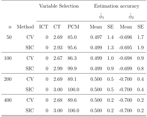
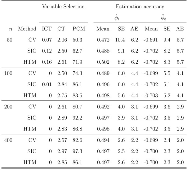
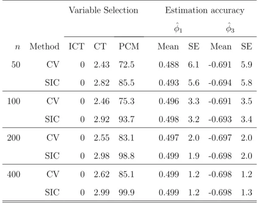
As stated in Ling (2005), with random errors from distributions satisfying (3.2) and (3.3), it can be shown theoretically that largerC would result in smaller asymp-totic variance of the SLAD estimator. However, a overly large C would make the dis-tribution of the SLAD estimator asymptotically non-normal even with a large sample size. Our simulation results show that with Cauchy errors, the empirical standard errors matched well with the asymptotical standard errors in the case of ρ = 90% but matched much worse in the case of ρ = 95%. However, when ǫi’s are from the S(1·5,0;1) distribution, bothρ= 90% andρ= 95% matched well. This indicates that the optimal choice of C varies for different models and error distributions to ensure that the conclusion of Theorem 3.2.1 still holds for the SLAD-alasso estimator.
not normal because of a poor choice of C, is it still possible for us to do the model selection using adaptive lasso? Fortunately, the answer is yes. Our simulation results indicate that the model selection result of slad-alasso becomes better asC increases. Particularly, if we takeCto be the 100% quantile ofyi’s, in which case we haveht= 1, the model selection results are the best. It motivates us to consider the ordinary least absolute deviation (LAD) as the loss function combining with the adaptive loss penalty function, which we name LAD-alasso. In the following subsection, we study the asymptotic property of LAD-alasso and explain why LAD-alasso performs better than SLAD-alasso in model selection in spite of the fact that the limiting distribution of the LAD-alasso estimator does not have a closed form.
3.2.3. Adaptive lasso with least absolute deviation
Denote L2n(φ) = Pnt=p+1|yt−XtTφ|, where Xt= (yt−1, . . . , yt−p)T. Define the LAD
estimator of Model (3.1) as ˜φ2n = arg minφ{L2n(φ)}. And then the LAD-alasso
estimator ˆφ1n is defined as the minimizer of
V2n(φ) =L2n(φ) +λnΣpj=1r2j|φj|, (3.8) where the weightr2j =|φ˜2j|−γ withγ >1 and ˜φ2j being thejth element of ˜φ2n. Note
that ˜φ1ncan be obtained by settingλn= 0 when minimizing (3.8). As stated in Davis et al. (1992), although Model (3.1) has an infinite variance and even infinite mean if α <1, the LAD estimator performs surprisingly well. In fact, ˜φ2n usually converges in a rate faster thann−1/2. In this sense, we obtain a better choice of weightsrj’s, and
hence for a given sample sizen, minimizing (3.8) would yield better variable selection results than that in the finite variance case.