OpenBU
http://open.bu.edu
Economics BU Open Access Articles
Fast algorithms for the quantile
regression process
This work was made openly accessible by BU Faculty. Please share how this access benefits you.
Your story matters.
Version
Citation (published version): Victor Chernozhukov, Ivan Fernandez-Val, Blaise Melly. "Fast
Algorithms for the Quantile Regression Process." ArXiv preprint,
Volume arXiv:1901.03821,
https://hdl.handle.net/2144/40243
arXiv:1909.05782v2 [econ.EM] 6 Apr 2020
(will be inserted by the editor)
Fast algorithms for the quantile regression process
Victor Chernozhukov · Iv´an Fern´andez-Val · Blaise Melly
Received: date / Accepted: date
Abstract The widespread use of quantile regression methods depends cru-cially on the existence of fast algorithms. Despite numerous algorithmic im-provements, the computation time is still non-negligible because researchers often estimate many quantile regressions and use the bootstrap for inference. We suggest two new fast algorithms for the estimation of a sequence of quantile regressions at many quantile indexes. The first algorithm applies the prepro-cessing idea of Portnoy and Koenker (1997) but exploits a previously esti-mated quantile regression to guess the sign of the residuals. This step allows for a reduction of the effective sample size. The second algorithm starts from a previously estimated quantile regression at a similar quantile index and up-dates it using a single Newton-Raphson iteration. The first algorithm is exact, while the second is only asymptotically equivalent to the traditional quantile regression estimator. We also apply the preprocessing idea to the bootstrap by using the sample estimates to guess the sign of the residuals in the bootstrap sample. Simulations show that our new algorithms provide very large improve-ments in computation time without significant (if any) cost in the quality of the estimates. For instance, we divide by 100 the time required to estimate 99 quantile regressions with 20 regressors and 50,000 observations.
Keywords Quantile regression·Quantile regression process·Preprocessing·
One-step estimator·Bootstrap·Uniform inference
V. Chernozhukov
Department of Economics, Massachusetts Institute of Technology, Cambridge, USA E-mail: [email protected]
I. Fern´andez-Val
Department of Economics, Boston University, Boston MA, USA E-mail: [email protected]
B. Melly
Department of Economics, University of Bern, Bern, Switzerland E-mail: [email protected]
1 Introduction
The idea of estimating regression parameters by minimizing the sum of ab-solute errors (i.e. median regression) predates the least squares method by about 50 years. Roger Joseph Boscovich suggested in 1857 to fit a straight line to observational data by minimizing the sum of absolute residuals under the restriction that the sum of residuals be zero. Laplace found in 1899 that
the solution to this problem is a weighted median.1 Gauss suggested later to
use the least squares criterion. For him, the choice of the loss function is an arbitrary convention and “it cannot be denied that Laplace’s convention vi-olates continuity and hence resists analytic treatment, while the results that my convention leads to are distinguished by their wonderful simplicity and generality.” Thus, it was mostly due to the simplicity of the analysis and of the computation that least squares methods have dominated the statistical
and econometric literature during two hundred years.2
Only the development of the simplex algorithm during the 20th century and its adaptation for median regression by Barrodale and Roberts (1974) made least absolute error methods applicable to multivariate regressions for problems of moderate size. Portnoy and Koenker (1997) developed an inte-rior points algorithm and a preprocessing step that significantly reduces the computation time for large samples with many covariates. These algorithms are implemented in different programming languages and certainly explain the surge of applications of quantile regression methods during the last 20 years.
Despite these improvements, the computation time is still non-negligible in two cases: when we are interested in the whole quantile regression process and when we want to use bootstrap for inference. Researchers are rarely inter-ested in only one quantile regression but often estimate many quantile regres-sions. The most common motivation for using quantile regression is, indeed, to analyze heterogeneity. Some estimation and inferential procedures even require the preliminary estimation of the whole quantile regression process. For instance, Koenker and Portnoy (1987) integrate the trimmed quantile re-gression process to get conditional trimmed means. Koenker and Xiao (2002),
Chernozhukov and Fern´andez-Val (2005) and Chernozhukov and Hansen (2006)
test functional null hypotheses such as the absence of any effect of a covariate or the location-scale model, which requires estimating the whole quantile re-gression process. Machado and Mata (2005) and Chernozhukov et al. (2013) must compute the whole quantile regression process to estimate the conditional distribution function by inverting the estimated conditional quantile function. In a second step, they integrate the conditional distribution function over the distribution of the covariates to obtain unconditional distributions.
In addition, researchers often use the bootstrap to estimate the standard errors of quantile regression. Many simulation studies show that it often pro-vides the best estimate of the variance of the point estimates. It also has the
1
Among others, see Chapter 1 in Stigler (1986). 2
See Koenker (2000) and Koenker (2017) for a more detailed historical account of the computation of median regression.
advantage of avoiding the (explicit) choice of a smoothing parameter, which is required for the analytical estimators of the variance. Finally, it is difficult to avoid the bootstrap (or other simulation methods) to test some types of functional hypotheses.
In these two cases, when the number of observations is large, the compu-tational burden of quantile regression may still be a reason not to use this method. In their survey of the decomposition literature, Fortin et al. (2011) mention the following main limitation of the quantile regression approach: “This decomposition method is computationally demanding, and becomes quite cumbersome for data sets numbering more than a few thousand ob-servations. Bootstrapping quantile regressions for sizeable number of quantiles
τ (100 would be a minimum) is computationally tedious with large data sets.”
Further improvements are clearly needed to enable more widespread applica-tions of quantile regression estimators.
In this paper we suggest two new algorithms to estimate the quantile re-gression process. The first algorithm is a natural extension of the preprocessing idea of Portnoy and Koenker (1997). The intuition is fairly simple. The fitted
quantile regression line interpolatesk data points, where k is the number of
regressors. Only the sign of the residuals of the other observations matters for the determination of the quantile regression coefficients. If one can guess the sign of some residuals, then these observations do not need to enter into the optimization problem, thus reducing the effective sample size. When many quantile regressions are estimated, then we can start with a conventional al-gorithm for the first quantile regression and then progressively climb over the conditional quantile function, using recursively the previous quantile regres-sion as a guess for the next one. This algorithm provides numerically the same estimate as the traditional algorithms because we can check if the guesses were correct and stop only if this is the case.
This algorithm seriously reduces the computation time when we estimate many quantile regressions. When these improvements are still insufficient, we suggest a new estimator for the quantile regression process. The idea consists in approximating the difference between two quantile regression coefficient vectors at two close quantile indexes using a first-order Taylor approximation. The one-step algorithm starts from one quantile regression estimated using one of the existing algorithms and then obtains sequentially all remaining quantile regressions using one-step approximations. This algorithm is extremely quick, but the estimates are numerically different from the estimates obtained using the other algorithms. Nevertheless, the one-step estimator is asymptotically equivalent to the standard quantile regression estimator if the distance between the quantile indexes decreases sufficiently fast with the sample size.
We also apply the preprocessing idea to compute the bootstrap estimates. When we bootstrap a quantile regression, we can use the sample estimates to guess the sign of the residuals in the bootstrap sample. With this algorithm, bootstrapping the quantile regression estimator is actually quicker than boot-strapping the OLS estimator. We cannot apply a similar approach to least squares estimators because of their global nature.
Instead of bootstrapping the quantile regression estimates, it is possible to bootstrap the score (or estimating equation) of the estimator. This ap-proach amounts in fact to using the one-step estimator to compute the boot-strap estimate when we take the sample estimate as a preliminary guess. This inference procedure, which has been suggested for quantile regression by Chernozhukov and Hansen (2006) and Belloni et al. (2017), is extremely fast and can also be used to perform uniform inference. Its drawback is the necessity to choose a smoothing parameter to estimate the conditional density of the response variable given the covariates.
The simulations we report in Section 6 show that the preprocessing
algo-rithm is 30 times faster than Stata’s built-in algoalgo-rithm when we have 50,000
observations, 20 regressors and we estimate 99 quantile regressions. The one-step estimator further divides the computing time by almost 4. The prepro-cessing step applied to the bootstrap of a single quantile regression divides the computing time by about 10. The score multiplier bootstrap further divides the computing time by 10 compared to the preprocessing algorithm. Thus, these new algorithms open new possibilities for quantile regression methods. For instance, in the application reported in Section 7, we could estimate 91
different quantile regressions in a sample of 2,194,021 observations, with 14
regressors and bootstrap 100 times the estimates in about 30 minutes on a laptop. The same estimation with the built-in commands of Stata would take over two months. The codes in Stata and some rudimentary codes in R are available from the authors.
We organize the rest of the paper as follows. Section 2 briefly defines the quantile regression model and estimator, describes the existing algorithms and provides the limiting distribution of the estimator. In Section 3, we adapt the preprocessing step of Portnoy and Koenker (1997) to estimate the whole quan-tile regression process. In Section 4, we suggest the new one-step estimator. Section 5 uses the same strategies to develop fast algorithms for bootstrap. Section 6 and 7 provide the results of the simulations and of the application, respectively. Finally, in Section 8 we point out some directions of research that may be fruitful.
2 The quantile regression process
This section gives a very brief introduction to the linear quantile regression model. For a more thorough discussion we recommend the book written by Koenker (2005) and the recent Handbook of Quantile Regression (Koenker et al., 2017).
2.1 The quantile regression model
We are often interested in learning the effect of a k×1 vector of covariates
LetQY(τ|x) be theτ conditional quantile ofY givenX =xwith 0< τ <1.
The conditional quantile function of Y given X, τ 7→ QY (τ|X), completely
describes the dependence between Y and X. For computational convenience
and simplicity of the interpretation, we assume that the conditional quantile functions are linear inx:
Assumption 1 (Linearity)
QY (τ|x) =x′β(τ)
for allτ ∈ T, which is a closed subset of[ε,1−ε]for some0< ε <1.
In this paper we focus on central quantile regression and suggest inference procedures justified by asymptotic normality arguments. Therefore, we must
exclude the tail regions. For extremal quantile regressions Chernozhukov and Fern´andez-Val
(2011) have suggested alternative inference procedures based on extreme value approximations. As a rule of thumb for continuous regressors, they suggest that normal inference performs satisfactorily if we setε= 15·k/n.
Most existing sampling properties of the quantile regression estimator have been derived for continuous response variables. Beyond the technical reasons for this assumption, the linearity assumption for the conditional quantile func-tions is highly implausible for discrete or mixed discrete-continuous response variables. Therefore, we impose the following standard assumption:
Assumption 2 (Continuity) The conditional density functionfY(y|x)
ex-ists, is uniformly continuous in (y, x)and bounded on the support of (Y, X).
For identification reasons, we require that the (density weighted) covariates are not linearly dependent:
Assumption 3 (Rank condition) The minimal eigenvalue of the Jacobian matrix J(τ) := E[fy(X′β(τ)|X)XX′)] is bounded away from zero uniformly
overτ∈ T.
Finally, we must impose a condition on the distribution of the covariates:
Assumption 4 (Distribution of the covariates) EkXk2+ε<∞for some
ε >0.
Assumptions 3 and 4 impose that the derivatives of the coefficient function
τ7→β(τ) are bounded uniformly onT because, by simple algebra (e.g., proof
of Theorem 3 in Angrist et al. (2006)), dβ(τ)
dτ =J(τ)
−1E(X). (1)
Under the linearity and the continuity assumptions, by the definition of
the quantile function, the parameter β(τ) satisfies the following conditional
moment restriction:
P(Y ≤x′β(τ)
It can be shown thatβ(τ) is the unique solution to the following optimiza-tion problem:
β(τ) = arg min
b∈Rk
E[ρτ(Y −X′b)] (3)
whereρτ is the check function defined asρτ(U) = (τ−1 (U ≤0))·U and 1 (·)
is the indicator function.3 The objective function is globally convex and its
first derivative with respect tobisE[(τ−1 (Y ≤X′b))X]. Thus,β(τ) solves
the unconditional moment condition
M(τ, β(τ)) :=E[(τ−1 (Y ≤X′β(τ)))X] = 0, (4)
which follows from the original conditional moment (2).
2.2 The quantile regression estimator
Let{yi, xi}ni=1be a random sample from{Y, X}. The quantile regression
esti-mator of Koenker and Bassett (1978) is the M-estiesti-mator that solves the sample analog of (3): b β(τ)∈arg min b∈Rk n X i=1 ρτ(yi−x′ib). (5)
This estimator is not an exact Z-estimator because the check function is not differentiable at 0. However, for continuous response variables, this will affect only thekobservations for whichyi=x′iβb(τ). Thus, the remainder term
van-ishes asymptotically and this estimator can be interpreted as an approximate Z-estimator: c Mτ,βb(τ):= 1 n n X i=1 τ−1yi≤x′iβb(τ) xi=op 1 √ n . (6)
The minimization problem (5) that βb(τ) solves can be written as a
con-vex linear program. This kind of problem can be relatively efficiently solved with some modifications of the simplex algorithm, see Barrodale and Roberts (1974), Koenker and D’Orey (1987) and Koenker and d’Orey (1994). The mod-ified simplex algorithm performs extremely well for problems of moderate size but becomes relatively slow in larger samples. Worst-case theoretical re-sults indicate that the number of iterations required can increase exponen-tially with the sample size. For this reason, Portnoy and Koenker (1997) have developed an interior point algorithm. Unlike the simplex, interior point al-gorithms start in the interior of the feasible region of the linear program-ming program and travel on a path towards the boundary, converging at the optimum. The inequality constraints are replaced by a barrier that pe-nalizes points that are close to the boundary of the feasible set. Since this barrier idea was pioneered by Ragnar Frisch and each iteration corresponds
3
to a Newton step, Portnoy and Koenker (1997) call their application of the interior point method to quantile regression the Newton-Frisch algorithm. Portnoy and Koenker (1997) have also suggested a preprocessing step that we will discuss in Section 3.
2.3 Sampling properties
For the sake of completeness we provide distribution theory for the quantile regression coefficient process. Following Angrist et al. (2006), we do not impose Assumption 1, therefore allowing for the possibility of model misspecification.
Proposition 1 (Asymptotic distribution theory) Under Assumptions 2 to 4, the quantile regression estimator defined in (5) is consistent for the pa-rameter defined in (3) uniformly over T. Moreover, the quantile regression processJ(·)√n(βb(·)−β(·))weakly converges to a zero mean Gaussian process
z(·)inℓ∞(T)k, whereℓ∞(T)is the set of bounded functions onT andz(·)is
defined by its covariance function
Σ(τ, τ′)
≡E[(τ−1 (Y ≤X′β(τ))) (τ′
−1 (Y ≤X′β(τ′)))XX′].
If the model is correctly specified, i.e. under Assumption 1, thenΣ(τ, τ′)
sim-plifies to
(min(τ, τ′)
−τ τ′)
·E[XX′].
Uniformly consistent estimators ofJ(τ) andΣ(τ, τ′) are useful for
analyt-ical inference and will be required to implement the one-step estimator and
the score bootstrap. We use the sample analog of Σ(τ, τ′) and Powell (1991)
kernel estimator ofJ(τ): b Σ(τ, τ′) = 1 n n X i=1 (τ−1(yi≤xi′βb(τ)))(τ′−1(yi≤x′iβb(τ′)))xix′i (7) b J(τ) = 1 n·hn n X i=1 K yi−xiβb(τ) hn ! xix′i (8)
where K(·) is a kernel function andhn is a bandwidth. We use a standard
normal density as kernel function and the Hall and Sheather (1988) bandwidth
hn=n−1/3·Φ−1 1−α22/3 " 1.5·φ Φ−1(τ)2 2·Φ−1(τ)2+ 1 #1/3 (9) whereφ(·) andΦ−1(·) are the density and quantile functions of the standard
normal andαis the targeted level of the test. These estimators are uniformly
consistent under the additional assumption thatEkXk4is finite. The pointwise
variance can consistently be estimated by
b
3 Preprocessing for the quantile regression process
3.1 Portnoy and Koenker (1997)
The fitted quantile regression line interpolates at least k data points. It can
easily be shown from the moment condition (6) that the quantile regression estimates are numerically identical if we change the values of the observations that are not interpolated as long as they remain on the same side of the regression line. The sign of the residuals yi−x′iβb(τ) is the only thing that
matters in the determination of the estimates. This explains why the quantile regression estimator is influenced only by the local behavior of the conditional distribution of the response near the specified quantile and is robust to outliers in the response variable if we do not go too far into the tails of the distribution.4
Portnoy and Koenker (1997) exploit this property to design a quicker
al-gorithm. Suppose for the moment that we knew that a certain subset JH of
the observations have positive residuals and another subsetJL have negative
residuals. Then the solution to the original problem (5) is exactly the same as the solution to the following revised problem
min
b∈RK
X
i /∈(JH∪JL)
ρτ(yi−xi′b) +ρτ(yL−x′Lb) +ρτ(yH−x′Hb) (11)
where xG = Pi∈JGxi, for G ∈ {H, L}, and yL, yH are chosen small and
large enough, respectively, to ensure that the corresponding residuals remain negative and positive. Solving this new problem gives numerically the same estimates but is computationally cheaper because the effective sample size is
reduced by the number of observations inJH andJL.
In order to implement this idea we need to have some preliminary infor-mation about the sign of some residuals. Portnoy and Koenker (1997) suggest to use only a subsample to estimate an initial quantile regression that will be used to guess the sign of the residuals in the whole sample. More formally, their algorithm works as follows:
Algorithm 1 (Portnoy and Koenker (1997))
1. Solve the quantile regression problem (5) using only a subsample of size
(k·n)2/3 from the original sample. This delivers a preliminary estimate
˜
β(τ).
2. Calculate the residuals ri =yi−xi′β˜(τ) and zi, a quickly computed
con-servative estimate of the standard error of ri. Calculate the τ − M2n and τ +2Mn quantiles of ri
zi. The observations below this first quantile are
in-cluded in JL; the observations above this second quantile are included in JH; theM =m·(k·n)2/3observations between these quantiles are kept for
the next step. mis a parameter that can be chosen by the user; by default it is set to0.8.
4
On the other hand, note that quantile regression is not robust to outliers in the x-direction.
3. Solve the modified problem (11) and obtainβb(τ)
4. Check the residual signs of the observations inJL andJH:
(a) If no bad signs (or the number of bad signs is below the number of allowed mispredicted signs),βb(τ)is the solution.
(b) If less than 0.1·M bad signs: take the observations with mispredicted sign out of JL andJH and go back to step 3.
(c) If more than0.1·M bad signs: go back to step 1 with a doubled subsample size.
Formal computational complexity results in Portnoy and Koenker (1997) indicate that the number of computation required by the simplex is quadratic in n, by the interior point method is of ordernk3log2
n, and by the
prepro-cessing algorithm is of ordern2/3k3log2
n+nk2.
3.2 Preprocessing for the quantile regression process
In many cases, the researcher is interested in the quantile regression coeffi-cients at several quantiles. This allows analyzing the heterogeneity of behavior, which is the main motivation for using quantile regression. For instance, it is common to estimate 99 quantile regressions, one at each percentile, and plot the estimated coefficients. Tests of functional hypotheses such as those
sug-gested in Koenker and Xiao (2002), Chernozhukov and Fern´andez-Val (2005)
and Chernozhukov and Hansen (2006) necessitate the estimation of a large number of quantile regressions. Some estimators also require the prelimi-nary estimation of the whole quantile regression process, such as the esti-mators suggested in Koenker and Portnoy (1987), Machado and Mata (2005) and Chernozhukov et al. (2013).
In the population we can let the quantile indexτincrease continuously from
0 to 1 to obtain a continuous quantile regression coefficient process. In finite samples, however, only a finite number of distinct quantile regressions exists.
In the univariate case, there are obviously only ndifferent sample quantiles.
In the general multivariate case, the number of distinct solutions depends on the specific sample but Portnoy (1991) was able to show that the number
of distinct quantile regressions is of order Op(nlogn) when the number of
covariates is fixed. Koenker and D’Orey (1987) provides an efficient parametric linear programming algorithm that computes the whole quantile regression
process.5 Given βb(τ), a single simplex pivot is required to obtain the next
quantile regression estimates. This is a feasible solution when n and k are
not too large but it is not feasible to compute Op(nlogn) different quantile
regressions in the type of applications that we want to cover. Therefore, we do not try to estimate the whole quantile regression process. Instead, we discretize the quantile regression process and estimate quantile regressions only on a grid of quantile indexes such asτ = 0.01,0.02, ...,0.98,0.99.
5
Parametric programming is a technique for investigating the effects of a change in the parameters (here of the quantile indexτ) of the objective function.
In order to approximate well enough the conditional distribution, several estimators requires that the mesh width of the grid converges to 0 at the
n−1/2 rate or faster.6 Neocleous and Portnoy (2008) show that it is enough
to estimate quantile regressions on a grid with a mesh width of order n−1/4
if we linearly interpolates between the estimated conditional quantiles and an additional smoothness condition is satisfied (the derivative of the conditional density must be bounded). Thus, interpolation may be used in a second step to improve the estimated conditional quantile function but even in this case a significant number of quantile regressions must be estimated.
At the moment, when a researcher wants to estimate 99 quantile regres-sions, she must estimate them separately and the computation time will be 99
times longer than the time needed for a single quantile regression.7We build
on the preprocessing idea of Portnoy and Koenker (1997) and suggest an algo-rithm that exploits recursively the quantile regressions that have already been
estimated in order to estimate the next one.8
Assume we want to estimateJ different quantile regressions at the quantile
indexesτ1< τ2< ... < τJ.
Algorithm 2 (Preprocessing for the quantile regression process)
To initialize the algorithm, βb(τ1) is estimated using one of the traditional
algorithms described above. Then, iteratively forj = 2, ..., J: 1. Useβb(τj−1)as a preliminary estimate.
2. Calculate the residuals ri = yi−x′iβb(τj−1) and zi, a quickly computed
conservative estimate of the standard error ofri. Calculate theτ−2Mn and τ+M2n quantiles of ri
zi. The observations below this first quantile are included
inJL; the observations above this second quantile are included in JH; the M = m·(k·n)1/2 observations between these quantiles are kept for the next step. mis a parameter that can be chosen by the user; by default it is set to 3.
3. Solve the modified problem (11) and obtainβb(τj)
4. Check the residual signs of the observations inJL andJH:
(a) If no bad signs (or the number of bad signs is below the number of allowed mispredicted signs),βb(τj) is the solution.
(b) If less than 0.1·M bad signs: take the observations with mispredicted sign out of JL andJH and go back to step 3.
(c) If more than 0.1·M bad signs: go back to step 2 with a doubled m.
Compared to Algorithm 1, the preliminary estimate does not need to be
computed because we can take the already computed βb(τj−1). This will
nat-urally provide a good guess of the sign of the residuals only ifτj andτj−1 are
6
See e.g. Chernozhukov et al. (2013). 7
It is actually possible to use the estimates from the previous quantile regression as start-ing values for the next quantile regression. These better startstart-ing values allow for reducstart-ing the computing time and are, therefore, used by all our algorithms.
8
In his comment of Portnoy and Koenker (1997), Thisted (1997) suggests this idea, which has never been implemented to the best of our knowledge.
close. This can be formalized by assuming that√n(τj−τj−1) =Op(1). When
this condition is satisfied, then√n(βb(τj)−βb(τj−1)) =Op(1) by the
stochas-tic equicontinuity of the quantile regression coefficient process. This justifies keeping a smaller sample in step 2: while we kept a sample proportional to
n2/3 in Algorithm 1, we can keep a sample proportional ton1/2 in Algorithm
2.
These two differences (no need for a preliminary estimate and smaller sam-ple size in the final regression) both imply that Algorithm 2 is faster than Al-gorithm 1 and should be preferred when a large number of quantile regressions is estimated. Finally, note that step 4 of both algorithms makes sure that the estimates are numerically equal (or very close if we allow for a few mispre-dicted signs of the residuals) to the estimates that we would obtain using the simplex or interior point algorithms. Thus, there is no statistical trade-off to consider when deciding which algorithm should be used. This decision can be based purely on the computing time of the algorithms. In the next section, we will consider an even faster algorithm but it will not provide numerically identical estimates. This new estimator will be only asymptotically equivalent to the traditional quantile regression estimator that solves the optimization problem (5).
4 One-step estimator
One-step estimators were introduced for their asymptotic efficiency by Le Cam (1956). A textbook treatment of this topic can be found in Section 5.7 of van der Vaart (1998). The one-step method builds on and improves a
prelim-inary estimator. If this prelimprelim-inary estimator is already √n-consistent, then
the estimator that solves a linear approximation to the estimating equation is asymptotically equivalent to the estimator that solves the original estimating
equation. In other words, when we start from a √n-consistent starting value,
then a single Newton-Raphson iteration is enough. Further iterations do not improve the first-order asymptotic distribution.
In this section we suggest a new estimator for the quantile regression coef-ficient process. This estimator is asymptotically equivalent to the estimators presented in the two preceding sections but may differ in finite samples. The idea consists in starting from one quantile regression computed using a stan-dard algorithm and then obtaining sequentially the remaining regression
coef-ficients using a single Newton-Raphson iteration for each quantile regression.9
In other words, this is a one-step estimator that uses a previously estimated
quantile regression for a similar quantileτ as the preliminary estimator.
Assume that we have already obtainedβb(τ1), a√n-consistent estimator of β(τ1), and we would like to obtainβb(τ1+ε) for a smallε. Formally, we assume
thatε=O(n−1/2) such thatβb(τ
1) is√n-consistent forβ(τ1+ε) because, by
9
We start from the median regression in the simulations and application in Sections 6 and 7.
the triangle inequality, kβb(τ1)−β(τ1+ε)k ≤ kβb(τ1)−β(τ1)k+ sup τ1≤τ′≤τ1+ε dβ(τ ′) dτ ε=OP(n−1/2)
where the last equality follows from (1) together with Assumptions 3 and 4. Then, by Theorem 5.45 in van der Vaart (1998) the one step estimator
b
β(τ1+ε) =βb(τ1)−Jb(τ1)−1M
τ1+ε,βb(τ1)
has the same first-order asymptotic distribution as the quantile regression estimator ofβ(τ1+ε). Here we use that
kJb(τ1)−J(τ1+ε)k ≤ kJb(τ1)−J(τ1)k+kJ(τ1)−J(τ1+ε)k →P 0,
by the triangle inequality, Assumptions 2 and 4, standard regularity conditions for Jb(τ1)→P J(τ1), and ε → 0. Note that the previous argument holds for
anyτ1, τ1+ε∈ T such thatε=O(n−1/2).
The one-step estimator corresponds to a single Newton-Raphson iteration. It is possible to use the resulting value as the new starting value for a second iteration and so on, but the first-order asymptotic distribution does not change. If we iterate until convergence, then
J(τ1)−1M
τ1+ε,βb(τ1+ε)
= 0
Since Jb(τ1) is asymptotically full rank by Assumption 3, this implies that
the moment condition (6) must be satisfied at τ1+ε such that we obtain
numerically the same values as the traditional quantile regression estimator of
β(τ1+ε). This property, together with the fact that the quantile regression
estimate is constant over a small range of quantile indexes, also implies that we can get numerically identical estimates to the traditional quantile regression
estimator by choosingεto be small enough. This is, however, not the objective
because the computation time of such a procedure would necessarily be higher
than that of the parametric linear programming algorithm.10
The algorithm is summarized below:
Algorithm 3 (One-step estimator for the quantile regression process)
To initialize the algorithm, βb(τ1) is estimated using one of the traditional
algorithms described above. Then, iteratively forj = 2, ..., J: 1. Useβb(τj−1)as a preliminary estimate.
2. Estimate the Jacobian matrix with Powell (1991) estimator and Hall and Sheather (1988) bandwidth and obtain Jb(τj−1).
10
Schmidt and Zhu (2016) have suggested a different iterative estimation strategy. They also start from one quantile regression but they add or subtract sums of nonnegative func-tions to it to calculate other quantiles. Their procedure has a different objective (monotonic-ity of the estimated conditional quantile function) and their estimator is not asymptotically equivalent to the traditional quantile regression estimator.
3. Update the quantile regression coefficient b β(τj) =βb(τj−1)−Jb(τj−1)−1 1 n n X i=1 τj−1 yi≤xiβb(τj−1) (12) The one-step estimator is much faster to compute when we do not choose a too fine grid of quantiles. Our simulations reported in Section 6 show that
a grid with ε = 0.01 works well even for large samples. This result depends
naturally on the data generating process. A fine grid may be needed when the
conditional density ofY is changing quickly (i.e. when the first order
approx-imation error is large). In practice, it is possible to estimate a few quantile regressions with the traditional estimator and check that the difference be-tween both estimators is small.
5 Fast algorithms for bootstrap inference
Researchers have often found that the bootstrap is the most reliable method for both pointwise and uniform inference. Naturally, this method is also the most demanding computationally. The time needed to compute the estimates can be a binding constraint when researchers are considering bootstrapping strategies. Fortunately, the same approaches that we have presented in the preceding sections (preprocessing and linear approximations) can also fruitfully reduce the computing time of the bootstrap.
5.1 Preprocessing for the bootstrap
A very simple modification of the preprocessing algorithm of Portnoy and Koenker (1997) leads to significant improvements. The advantage when we compute a quantile regression for a bootstrap sample is that we can use the already com-puted estimate in the whole sample to guess the sign of the residuals. This means that we can skip step 1 of the preprocessing Algorithm 1. In addition, this preliminary estimate is more precise because it was computed using a sample of size n instead of (k·n)2/3 in the original preprocessing algorithm. Thus, we need only to keep a lower number of observations in step 2. We
chooseM =m·(k·n)1/2where mis set by default to 3 but can be modified
by the user. This multiplying constant 3 was chosen because it worked well in our simulations. We do not have a theoretical justification for this choice and further improvements should be possible. In particular, it should be possible to adjust this constant during the process (that is after the estimates in a few bootstrap samples have been computed) by increasing it when the sign of too many residuals is mispredicted in step 4 or decreasing it when the sign of the
residuals is almost never mispredicted.11
11
A similar idea could be applied to adjust the constantmin Algorithm 2. The additional difficulty is that the optimal constant probably depends on the quantile indexτ, which is not the case for the bootstrap.
We now define formally the algorithm for the empirical bootstrap but a similar algorithm can be applied to all types of the exchangeable bootstrap.
Algorithm 4 (Preprocessing for the bootstrap)
For each bootstrap iterationb= 1, ..., B, denote by {y∗b
i , x∗ib}ni=1 the bootstrap
sample:
1. Useβb(τ)as a preliminary estimate. 2. Calculate the residuals r∗b
i =yi∗b−xi∗b′βb(τ) and zi∗b, a quickly computed
conservative estimate of the standard error of r∗b
i . Calculate the τ− M2n
andτ+2Mn quantiles of r∗
b i
z∗b
i . The observations below this first quantile are
included inJL; the observations above this second quantile are included in JH; theM =m·(k·n)1/2observations between these quantiles are kept for
the next step.mis a parameter that can be chosen by the user; by default it is set to3.
3. Solve the modified problem (11) for the sample {y∗b
i , x∗ib}ni=1and obtain
b
β∗b(τ).
4. Check the residual signs of the observations inJL andJH:
(a) If no bad signs (or the number of bad signs is below the number of allowed mispredicted signs),βb∗b(τ), is the solution.
(b) If less than 0.1·M bad signs: take the observations with mispredicted sign out of JL andJH and go back to step 3.
(c) If more than 0.1·M bad signs: go back to step 2 with a doubled m.
With this algorithm, bootstrapping a single quantile regression becomes
faster than bootstrapping the least squares estimator. The preprocessing strat-egy does not apply to least squares estimators because of the global nature of these estimators.
When the whole quantile regression process is bootstrapped, either
Algo-rithm 2 or AlgoAlgo-rithm 4 can be applied.12 In our simulations we found that
the computing times were similar for these two algorithms. In our implemen-tation, Algorithm 4 is used in this case. Even shorter computing times can be obtained either by using the one-step estimator in each bootstrap sample or by bootstrapping the linear representation of the estimator, which we will present in the next subsection. These two algorithms are not numerically iden-tical to the traditional quantile regression estimator and require the choice of a smoothing parameter to estimate the Jacobian matrix.
5.2 Score resampling (or one-step bootstrap)
Even with the preprocessing of Algorithm 4, we must recompute the esti-mates in each bootstrap draw, which is naturally computationally demanding.
12
Algorithm 2 can be slightly improved by using preprocessing with ˆβ(τ1) as a preliminary estimate of ˆβ∗b
Instead of resampling the covariates and the response to compute the coeffi-cients, we can resample the asymptotic linear (Bahadur) representation of the estimators. Belloni et al. (2017) suggest and prove the validity of the
multi-plier score bootstrap. Forb= 1, ..., B we obtain the corresponding bootstrap
draw ofβb(τ) via b β∗b(τ) =βb(τ) −Jb(u)−1 1 n n X i=1 ξ∗b i τ−1yi≤x′iβb(τ) (13) where ξ∗b i n
i=1 are iid random variables that are independent from the data
and must satisfy the following restrictions:
Eξ∗b i = 0 andV ar ξixb = 1.
We have implemented this score multiplier bootstrap for three different dis-tributions of ξ∗b
i (i) ξi∗b ∼ E −1 where E is a standard exponential random
variable, which corresponds to the Bayesian bootstrap (see e.g. Hahn (1997)), (ii)ξ∗b
i ∼N(0,1), which corresponds to the Gaussian multiplier bootstrap (see
e.g. Gin´e et al. (1984)), (iii)ξ∗b
i ∼N1/√2 + N22−1
/2 whereN1andN2are
mutually independent standard normal random variables, which corresponds to the wild bootstrap (see e.g. Mammen et al. (1993)). In addition to the mul-tiplier bootstrap, we have also implemented the score bootstrap suggested in Chernozhukov and Hansen (2006), which corresponds to (13) with multino-mial weights. Since these different distributions give very similar results, we report only the performance of the wild score bootstrap in the simulations in Section 6.
The score resampling procedure can be interpreted as a one-step estimator of the bootstrap value where we use the sample estimate as the preliminary value. This interpretation can be seen by comparing equation (12) with equa-tion (13). Kline and Santos (2012) notice this connecequa-tion between the score bootstrap and one-step estimators in their remark 3.1.
While the score bootstrap is much faster to compute than the exchangeable
bootstrap, it requires the preliminary estimation of the matrix J(τ). This
matrix is a function offY(X′β(τ)|X), which is relatively difficult to estimate
and necessitates the choice of a smoothing parameter. Thus, the multiplier bootstrap has no advantage in this respect compared to analytical estimators of the pointwise standard errors. On the other hand, the score bootstrap can be used to test functional hypotheses within relatively limited computing time (see Chernozhukov and Hansen (2006) for many examples).
To summarize, for bootstrapping the quantile regression process we can recompute the estimate in each bootstrap draw and each quantile using pre-processing as introduced in Section 5.1. Alternatively, we can use a first-order approximation starting from another quantile regression in the same bootstrap sample (one-step estimator) or we can use a first-order approximation starting from the sample estimate at the same quantile (score resampling). The simu-lations in the following section will compare these different approaches both in term of computing time as in term of the quality of the inference.
6 Simulations
The results in Sections 6 and 7 were obtained using Stata 14.2. We compare the official Stata command (qreg), which implements a version of the simplex algorithm according to the documentation, with our own implementation of the other algorithms directly in Stata. The codes and the data to replicate these results are available from the authors. The reference machine used for all the simulations is an AMD Ryzen Threadripper 1950X with 16 cores at 3.4 GHz and 32 GB of RAM (but for each simulation each algorithm exploits only one processor, without any parallelism).
6.1 Computation times
We use empirical data to simulate realistic samples. We calibrate the data generating processes to match many characteristics of a Mincerian wage re-gression. In particular, we draw covariates (such as education in years and as a set of indicator variables, a polynomial in experience, regional indica-tor variables, etc.) from the Current Population Survey data set from 2013. We consider different sets of regressors with dimensions ranging from 8 to 76. Then, we simulate the response variable by drawing observations from the estimated conditional log wage distribution.
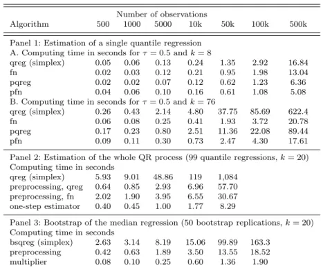
Table 1 provides the average computing times (over 200 replications) for three different cases. In the first panel, we compare different algorithms to estimate a single quantile regression.13It appears that the interior point
algo-rithm (denoted by fn in the table) is always faster than the simplex algoalgo-rithm as implemented by Stata. Preprocessing (denoted by pfn and pqreg) becomes an attractive alternative when the number of observations is ‘large enough’,
where ‘large enough’ corresponds to 5,000 observations when there are 8
re-gressors but 500,000 observations when there are 76 regressors. In this last
configuration (n = 500,000 and k = 76) the computing time needed by the
interior point algorithm with the preprocessing step is 35 times lower than the computing time of the built-in Stata’s command. The improvement in this first panel is only due to the implementation of algorithms suggested by Portnoy and Koenker (1997). All these estimators provide numerically identi-cal estimates.
The second panel of Table 1 compares the algorithms when the objective is to estimate 99 different quantile regressions, one at each percentile. For all sample sizes considered the algorithm with the preprocessing step suggested in Section 3.2 computes the same estimates at a fraction of the computing
time of the official Stata command. Whenn= 50,000, the computing time is
divided by more than 50. The one-step estimator defined in Section 4 further divides the computing time by a factor of about 4. Since this estimator is only
13
We provide the results for the median regression but the ranking was similar at other quantile indexes.
Table 1. Comparison of the algorithms
Number of observations
Algorithm 500 1000 5000 10k 50k 100k 500k
Panel 1: Estimation of a single quantile regression A. Computing time in seconds forτ= 0.5 andk= 8
qreg (simplex) 0.05 0.06 0.13 0.24 1.35 2.92 16.84
fn 0.02 0.03 0.12 0.21 0.95 1.98 13.04
pqreg 0.02 0.02 0.07 0.12 0.62 1.23 6.36
pfn 0.04 0.06 0.10 0.16 0.61 1.08 5.08
B. Computing time in seconds forτ= 0.5 andk= 76
qreg (simplex) 0.26 0.43 2.14 4.80 37.75 85.69 622.4
fn 0.06 0.08 0.25 0.41 1.93 3.72 20.78
pqreg 0.17 0.23 0.80 2.51 11.36 22.08 89.44
pfn 0.09 0.11 0.30 0.73 2.47 4.30 17.61
Panel 2: Estimation of the whole QR process (99 quantile regressions,k= 20) Computing time in seconds
qreg (simplex) 5.93 9.01 48.86 119 1,084 preprocessing, qreg 0.64 0.85 2.93 6.96 57.70 preprocessing, fn 2.02 1.90 3.95 6.55 30.67 one-step estimator 0.40 0.45 1.00 1.77 8.29
Panel 3: Bootstrap of the median regression (50 bootstrap replications,k= 20) Computing time in seconds
bsqreg (simplex) 2.63 3.14 8.19 15.06 99.89 163.3 preprocessing 0.42 0.63 1.89 3.50 13.55 18.52 multiplier 0.08 0.10 0.25 0.60 1.36 1.90 Note: Average computing times over 200 replications.
asymptotically equivalent to the other algorithms, we also measure its perfor-mance compared to the traditional quantile regression estimator in Subsection 6.2.
In the third panel of Table 1 we compare the computing time needed to bootstrap 50 times the median regression with the official Stata command, with the preprocessing step introduced in Section 5.1 and with the score boot-strap described in Section 5.2. The results show that the preprocessing step divides the computing time by about 4 for small sample sizes and by 9 for the largest sample size that we have considered. Using the multiplier bootstrap di-vides the computing time one more time by a factor of 10. However, this type of bootstrap is not numerically identical to the previous ones. The simulations in the subsections 6.3 and 6.4 show that it tends to perform slightly worse in small samples.
6.2 Performance of the one-step estimator
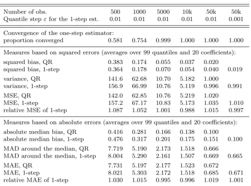
Table 2 and Figure 1 measure the performance of the one-step estimator. We use the same data generating process as in the previous subsection with
k = 20 regressors. We perform 10,000 replications to get precise results. We first note that the one-step algorithm sometimes does not converge. The reason is thatJb(τ) is occasionally singular or close to singular in small samples. As a consequence, the one-step estimateβb(τ+ε), which is linear inJb(τ)−1, takes
a very large value. Once the estimated quantile regression coefficients at one quantile index are very far away from the true values, then the JacobianJb(τ) and the coefficients at the remaining quantile indices will be very far from the true values. It would be possible to detect convergence issues by checking that the moment conditions are approximately satisfied or by estimating a few quantile regressions with a traditional algorithm and checking that the estimates are close. We did not yet implement this possibility because the
convergence problem appears only in small samples (when n ≤ 1000) and
traditional algorithms are anyway fast enough for these sample sizes.
Our parameters of interest are the 20×1 vectors of quantile regression
co-efficients at the quantile indicesτ = 0.01,0.02, ...0.99. Thus, in principle, there are 1980 different parameters of interest and we could analyze each of them separately. Instead, we summarize the results and report averages (over
quan-tile indices and regressors) of several measures of performance in Table 2.14In
Figure 1 we plot the main measure separately for each quantile (but averaged over the regressors since the results are similar for different regressors). The second part of Table 2 reports the standard measures of the performance of an estimator: squared (mean) bias, variance, and mean squared error (MSE). Since these measures based on squared errors are very sensitive to outliers, in the third part of the table, we also report measures based on absolute devi-ations: the absolute median bias, median absolute deviation (MAD) around the median, and median absolute error (MAE) around the true value.
The bias of the one-step estimator is slightly larger than the bias of the traditional estimator in small and moderate sample sizes but it contributes
only marginally to the MSE and MAE because it is small. When n = 500,
the MAE (MSE) of the one-step estimator is on average 3% (8.7%) higher
than the MAE (MSE) of the traditional quantile regression estimator. These disadvantages converge quickly to 0 when the sample size increases and are
negligible when we have at least 5,000 observations. Thus, the one-step
es-timator performs well exactly when we need it, i.e. when the sample size is large and computing the traditional quantile regression estimator may take too much time.
In the last column of Table 2, we can assess the role of ε, the distance
between quantile indices. In the first 6 columns, we useε= 0.01 and estimate
99 quantile regressions for τ = 0.01,0.02, ...,0.99. To satisfy the conditions 14
To make the estimates comparable across quantiles and regressors, we first normalize them such that they have unit variance in the specification with n= 50,000. Then, we calculate the measures of performance separately for each parameter and average them over all quantile indices and regressors. The reported relative MSE and MAE are the averaged relative MSE and MAE. Alternatively, it is possible to calculate the ratio of the averaged MSE and MAE with the results in Table 2. These ratios of averages and averages of ratios are very similar.
Table 2. Performance of the one-step estimator
Number of obs. 500 1000 5000 10k 50k 50k
Quantile stepεfor the 1-step est. 0.01 0.01 0.01 0.01 0.01 0.001 Convergence of the one-step estimator:
proportion converged 0.581 0.754 0.999 1.000 1.000 1.000 Measures based on squared errors (averages over 99 quantiles and 20 coefficients): squared bias, QR 0.383 0.174 0.055 0.037 0.020 squared bias, 1-step 0.364 0.178 0.070 0.054 0.040 0.019
variance, QR 141.6 62.68 10.70 5.182 1.000
variance, 1-step 156.9 66.99 10.76 5.119 0.996 0.991
MSE, QR 142.0 62.85 10.76 5.219 1.020
MSE, 1-step 157.2 67.17 10.83 5.173 1.035 1.010
relative MSE of 1-step 1.087 1.052 1.001 0.988 1.015 0.997 Measures based on absolute errors (averages over 99 quantiles and 20 coefficients): absolute median bias, QR 0.416 0.281 0.166 0.138 0.100 absolute median bias, 1-step 0.476 0.317 0.201 0.175 0.151 0.100 MAD around the median, QR 7.719 5.190 2.173 1.518 0.666 MAD around the median, 1-step 8.004 5.290 2.161 1.507 0.669 0.665
MAE, QR 7.731 5.197 2.177 1.523 0.672
MAE, 1-step 8.021 5.303 2.172 1.518 0.685 0.671
relative MAE of 1-step 1.030 1.015 0.995 0.996 1.019 1.001 Note: Statistics computed over 10,000 replications.
required to prove the asymptotic equivalence of the one-step and the
tradi-tional estimators, we should decrease ε when the sample size increases. The
fixed difference between quantile indices does not seem to prevent the relative
MAE and MSE of the one-step estimator to converge to 1 whenn= 10,000.
However, whenn= 50,000 we see a (slight) increase in the relative MSE and
MAE of the one-step estimator. Therefore, in the last column of the table,
we reduce the quantile step to ε = 0.001 and we see that the relative MAE
and MSE go back to 1 as predicted by the theory. Of course, the computing time increases when the quantile step decreases such that the researcher may prefer to pay a (small) price in term of efficiency to compute the estimates more quickly.
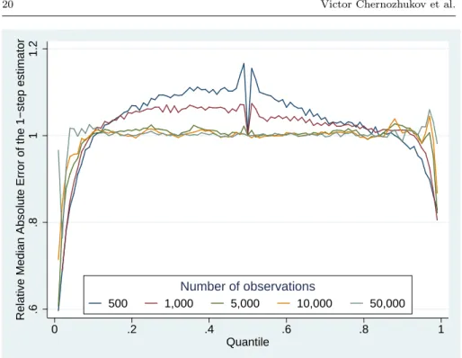
Figure 1 plots the relative MAE of the one-step estimator as a function of the quantile index. Remember that we initialize the algorithm at the me-dian such that both estimators are numerically identical at that quantile. With
500 or 1,000 observations, we nevertheless observe the largest relative MAE at
quantile indices close to the median. On the other hand, the one-step estimator is more efficient than the traditional estimator at the tails of the distribution. Given that the extreme quantile regressions are notoriously hard to estimate, we speculate that the one-step estimator may be able to reduce the estimation error by using implicitly some information from less extreme quantile
regres-.6
.8
1
1.2
Relative Median Absolute Error of the 1−step estimator
0 .2 .4 .6 .8 1
Quantile
500 1,000 5,000 10,000 50,000
Number of observations
Fig. 1. Relative MAE as a function of the quantile and the number of obser-vations
sions, similar to the extrapolation estimators for extreme quantile regression of Wang et al. (2012) and He et al. (2016). When the sample size increases, the curve becomes flatter and the relative MAE is very close to 1 at all quantiles between the first and ninth decile.
6.3 Pointwise inference
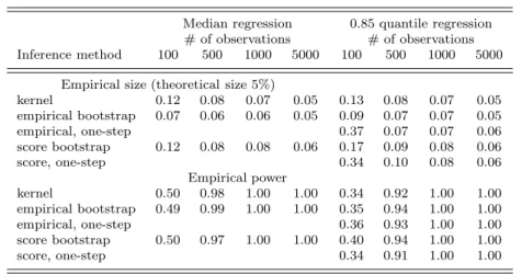
There exist several inference methods for quantile regression with very differ-ent computational burdens. In this subsection we compare the methods for pointwise inference and the next subsection the methods for uniform infer-ence. In both cases we simulate data from the same data generating process as Hagemann (2017):
yi=xi+ (0.1 +x2i)·ui (14)
where xi ∼N(0,1) andui ∼N(0,1/3). Table 3 provides the empirical
rejec-tion probabilities of a correct and of an incorrect null hypothesis about the coefficient on x2
i at a single quantile index. The intended statistical level of
the tests is 5%. We consider separately two different quantile indexesτ= 0.5
Table 3. Pointwise inference
Median regression 0.85 quantile regression # of observations # of observations Inference method 100 500 1000 5000 100 500 1000 5000
Empirical size (theoretical size 5%)
kernel 0.12 0.08 0.07 0.05 0.13 0.08 0.07 0.05 empirical bootstrap 0.07 0.06 0.06 0.05 0.09 0.07 0.07 0.05 empirical, one-step 0.37 0.07 0.07 0.06 score bootstrap 0.12 0.08 0.08 0.06 0.17 0.09 0.08 0.06 score, one-step 0.34 0.10 0.08 0.06 Empirical power kernel 0.50 0.98 1.00 1.00 0.34 0.92 1.00 1.00 empirical bootstrap 0.49 0.99 1.00 1.00 0.35 0.94 1.00 1.00 empirical, one-step 0.36 0.93 1.00 1.00 score bootstrap 0.50 0.97 1.00 1.00 0.40 0.94 1.00 1.00 score, one-step 0.34 0.91 1.00 1.00
We compare the following methods for inference: (i) the kernel estimator of the pointwise variance (10), which can be computed very quickly, (ii) the empirical bootstrap of the quantile regression coefficients that solves the full optimization problem (5) and is the most demanding in term of computation time, (iii) the empirical bootstrap of the one-step estimator (3), which uses a linear approximation in the quantile but not in the bootstrap direction, (iv) the score multiplier bootstrap based on the quantile regression estimator, which uses a linear approximation in the bootstrap but not in the quantile direction, (v) the score multiplier bootstrap based on the one-step estimator, which uses two linear approximations and is the fastest bootstrap implementation. Note that we have initialized the one-step estimator at the median such that there is no difference at the median but there can be a difference at the 0.85 quantile regression between the one-step and the original quantile regression estimators. In small samples all methods over-reject the correct null hypothesis but they all perform satisfactorily in large samples with empirical sizes that are very close to the theoretical size. The empirical bootstrap exhibits the lowest size distortion, which may warrant its higher computing burden. The ana-lytic kernel-based method and the score multiplier bootstrap perform very similarly; this is not a surprise because they should provide the same stan-dard errors when the number of bootstrap replications goes to infinity. Thus, there is no reason to use the score bootstrap when the goal is only to perform pointwise inference. The tests based on the one-step estimator displays a poor performance in very small samples. This is simply the consequence of the poor quality of the point estimates in very small samples that was shown in Table 2. Like for the point estimates, the performance improves quickly and becomes almost as good as the tests based on the original quantile regression estimator.
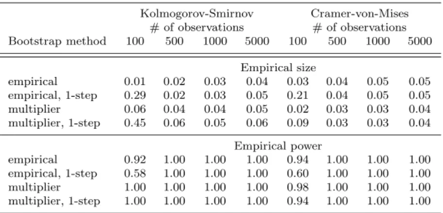
Table 4. Uniform inference
Kolmogorov-Smirnov Cramer-von-Mises # of observations # of observations Bootstrap method 100 500 1000 5000 100 500 1000 5000 Empirical size empirical 0.01 0.02 0.03 0.04 0.03 0.04 0.05 0.05 empirical, 1-step 0.29 0.02 0.03 0.05 0.21 0.04 0.05 0.05 multiplier 0.06 0.04 0.04 0.05 0.02 0.03 0.03 0.04 multiplier, 1-step 0.45 0.06 0.05 0.06 0.09 0.03 0.03 0.04 Empirical power empirical 0.92 1.00 1.00 1.00 0.94 1.00 1.00 1.00 empirical, 1-step 0.58 1.00 1.00 1.00 0.60 1.00 1.00 1.00 multiplier 1.00 1.00 1.00 1.00 0.98 1.00 1.00 1.00 multiplier, 1-step 1.00 1.00 1.00 1.00 0.94 1.00 1.00 1.00 6.4 Functional inferenceIn this subsection we evaluate the performance of the implemented procedures for uniform inference. We consider the same data generating process (14) and
test the null hypotheses that the coefficient on X is uniformly equal to 1
(this is true) and that the coefficient on X2 is uniformly equal to 0 (this is
false). We test these hypotheses with Kolmogorov-Smirnov (supremum of the
deviations from the null hypothesis over the quantile rangeT) and Cramer-von
Mises statistics (average deviation from the null hypothesis over the quantile
rangeT), both with Anderson-Darling weights. We estimate the critical values
using either the empirical bootstrap or the score bootstrap.15We estimate the
discretized quantile regression process for τ = 0.1,0.11,0.12, ...,0.9 and we report the results for a theoretical size of 5%.
Table 4 provides the results. Unsurprisingly, the one-step estimator forms badly with 100 observations. With this exception, all procedures per-form satisfactorily for both test statistics even for moderate sample sizes. Even the fastest procedure (multiplier bootstrap based on the one-step estimators) is reliable when the sample size includes at least 500 observations. This
opti-mistic conclusion may be due to the low number of parameters (k= 3) and to
the smoothness of the conditional distribution of the response variable..
7 An empirical illustration
In this section we update the results obtained by Abrevaya (2001) and Koenker and Hallock (2001) using data from June 1997. They utilized quantile regression to
ana-15
See Chernozhukov and Fern´andez-Val (2005), Angrist et al. (2006), Chernozhukov and Hansen (2006) and Belloni et al. (2017) for more details and proofs of the validity of these procedures.
lyze the effect of prenatal care visits, demographic characteristics and mother behavior on the distribution of birth weights. We use the 2017 Natality Data provided by the National Center for Health Statistics. Like Abrevaya (2001) and Koenker and Hallock (2001) we keep only singleton births, with mothers recorded as either black or white, between the ages of 18 and 45, residing in the United States. We also dropped observations with missing data for any of the regressors. This procedure results in a sample of 2,194,021 observations.
We regress the newborn birth weights in grams on a constant and 13 co-variates: gender of the newborn; race, marital status, education (4 categories), and age (and its square) of the mother; an indicator for whether the mother smoked during the pregnancy and the average number of cigarettes smoked per day; and the prenatal medical care of the mother divided in four categories. We estimate 91 quantile regressions forτ= 0.05,0.06, ...,0.95 and perform 100
bootstrap replications.16 Given the large number of observations, regressors,
quantile regressions and bootstrap replications, we use the fastest procedures, which is the one-step quantile regression estimator combined with the score multiplier bootstrap. The computation of all these quantile regressions and bootstrap simulations took about 30 minutes on a 4-cores processor cloked at 3.7 GHz, i.e. a relatively standard notebook. With the built-in Stata com-mands the computation of the same quantile regressions and bootstrap should take more than 2 months. The new algorithms clearly open new opportunities for quantile regression.
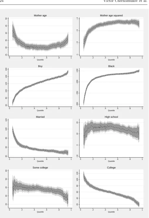
Figures 2 and 3 present the results for this example. For each coefficient, the line shows the point estimates, the dark grey area shows the 95% pointwise confidence intervals and the light grey area shows the 95% uniform confidence
bands, which are wider by construction.17Any functional null hypothesis that
lies outside of the uniform confidence band even at a single quantile can be rejected at the 5% level. For instance, it is obvious that none of the bands contains the value 0 at all quantiles. We can, therefore, reject the null hypoth-esis that the regressor is irrelevant in explaining birth weight for all included covariates. For all variables we can also reject the null hypothesis that the quantile regression coefficient function is constant (location-shift model) be-cause there is no value that is inside of the uniform bands at all quantiles.18On
the other hand, we cannot reject the location-scale null hypothesis for some covariates because there exists a linear function of the quantile index that is covered by the band. This is the case for instance for all variables measuring the education of the mother.
Birth weight is often used as a measure of infant health outcomes at birth. Clearly, a low birth weight is associated in the short-run with higher one-year
16
Due to computational limitations, Abrevaya (2001) and Koenker and Hallock (2001) used only the June subsample to estimate 5, respectively 15, different quantile regressions and they avoided bootstrapping the results. Of course, computers have become more pow-erful in the meantime.
17
See the supplementary appendix SA to Chernozhukov et al. (2013) for the construction and the validity of the uniform bands.
18
25 30 35 40 45 50 0 .2 .4 .6 .8 1 Quantile Mother age −1 −.8 −.6 −.4 0 .2 .4 .6 .8 1 Quantile Mother age squared
60 80 100 120 140 160 0 .2 .4 .6 .8 1 Quantile Boy −300 −250 −200 −150 0 .2 .4 .6 .8 1 Quantile Black 40 60 80 100 120 0 .2 .4 .6 .8 1 Quantile Married −10 0 10 20 0 .2 .4 .6 .8 1 Quantile High school 20 30 40 50 60 0 .2 .4 .6 .8 1 Quantile Some college 20 40 60 80 100 120 0 .2 .4 .6 .8 1 Quantile College
−600 −400 −200 0 0 .2 .4 .6 .8 1 Quantile No prenatal doctor visit
−20 −10 0 10 20 0 .2 .4 .6 .8 1 Quantile Medical care, 2nd trimester
−50 0 50 100 0 .2 .4 .6 .8 1 Quantile Medical care, 3rd trimester
−180 −160 −140 −120 −100 0 .2 .4 .6 .8 1 Quantile Mother smoked −10 −8 −6 −4 0 .2 .4 .6 .8 1 Quantile Cigarettes per day
1500 2000 2500 3000 3500 0 .2 .4 .6 .8 1 Quantile Intercept
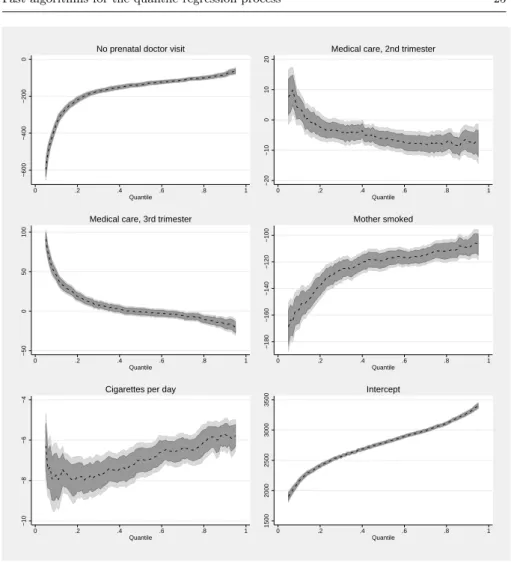
Fig. 3. Quantile regression estimates of the birth weight model (cont.)
mortality rates and in the longer run with worse educational attainment and earnings, see, e.g., Black et al. (2007). On the other hand, the goal of pol-icy makers is clearly not to maximize birth weights. In a systematic review, Baidal et al. (2016) find that higher birth weight was consistently associated with higher risk of childhood obesity. Thus, we do not want to report the aver-age effects of potential determinants of the birth weight but we need to analyze separately their effects on both tails of the conditional birth weight distribu-tion. In the location-shift model, the effect of the covariates is restricted to be the same over the whole distribution and it can be estimated by least-squares methods. But the homogeneity of the effects is rejected for all regressors such that we need quantile regression.
In light of this discussion, it is interesting to see that the effect of a higher mother education (especially of a college degree) is much higher at the lower end of the distribution where we want to increase the birth weight. Similarly, not seeing a doctor during the whole pregnancy has dramatic effect at the lower end of the distribution. While not recommended, not seeing a doctor has only mild effect at the top of the distribution. In general, the results are surprisingly similar to the results reported by Koenker and Hallock (2001) in their Figure 4. Twenty years later, the shape, the sign and even the magnitude of most coefficients are still similar.
8 Prospects
The advance of technology is leading to the collection of such a large amount of data that they cannot be saved or processed on a single computer. When this
is the case, Volgushev et al. (2019) suggest estimating separately J quantile
regressions on each computer and averaging these estimates. In a second step, they obtain the whole quantile process by using a B-spline interpolation of the estimated quantile regressions. We think that the new algorithms, in partic-ular the one-step estimator, can be useful for the distributed computation of the quantile regression process. The computation of the one-step estimator
re-quires only the communication of ak×1 vector and ak×kmatrix of sample
means, which can be averaged by the master computer. Thus, the one-step estimator can be implemented even when the data set must be distributed on several computers.
The optimization problem that defines the linear quantile regression esti-mator is actually easy to solve because it is convex. The optimization prob-lems defining, for instance, censored quantile regression, instrumental variable quantile regression, binary quantile regression are more difficult to solve by
several orders of magnitude because they are not convex.19 Estimating the
whole quantile process for these models may not be computationally feasible for the moment. It should be possible to adapt the suggested preprocessing and one-step algorithms to estimate the quantile processes also in these models. Acknowledgements We would like to thank the associate editor Roger Koenker, two annomynous referees, and the participants to the conference “Economic Applications of Quantile Regressions 2.0” that took place at the Nova School of Business and Economics for useful comments.
19
See Powell (1987) for the censored quantile regression estimator, Chernozhukov and Hansen (2006) for the instrumental variable quantile regression estimator and Kordas (2006) for the binary quantile regression estimator, which is a generalization of Manski (1975) maximum score estimator.
References
Abrevaya J (2001) The effects of demographics and maternal behavior on the distribution of birth outcomes. Empirical Economics 26(1):247–257
Angrist J, Chernozhukov V, Fern´andez-Val I (2006) Quantile regression under
misspecification, with an application to the us wage structure. Econometrica 74:539–563
Baidal JAW, Locks LM, Cheng ER, Blake-Lamb TL, Perkins ME, Taveras EM (2016) Risk factors for childhood obesity in the first 1,000 days: a systematic review. American journal of preventive medicine 50(6):761–779
Barrodale I, Roberts F (1974) Solution of an overdetermined system of equa-tions in the l 1 norm [f4]. Communicaequa-tions of the ACM 17(6):319–320
Belloni A, Chernozhukov V, Fern´andez-Val I, Hansen C (2017) Program
evaluation and causal inference with high-dimensional data. Econometrica 85(1):233–298
Black SE, Devereux PJ, Salvanes KG (2007) From the cradle to the labor market? the effect of birth weight on adult outcomes. The Quarterly Journal of Economics 122(1):409–439
Chernozhukov V, Fern´andez-Val I (2005) Subsampling inference on quantile
regression processes. Sankhya: The Indian Journal of Statistics 67:253–276
Chernozhukov V, Fern´andez-Val I (2011) Inference for extremal conditional
quantile models, with an application to market and birthweight risks. The Review of Economic Studies 78(2):559–589
Chernozhukov V, Hansen C (2006) Instrumental quantile regression inference for structural and treatment effect models. Journal of Econometrics 132:491– 525
Chernozhukov V, Fern´andez-Val I, Melly B (2013) Inference on counterfactual
distributions. Econometrica 81(6):2205–2268
Fortin N, Lemieux T, Firpo S (2011) Decomposition methods in economics. In: Handbook of labor economics, vol 4, Elsevier, pp 1–102
Gin´e E, Zinn J, et al. (1984) Some limit theorems for empirical processes. The Annals of Probability 12(4):929–989
Hagemann A (2017) Cluster-robust bootstrap inference in quantile regression models. Journal of the American Statistical Association 112(517):446–456 Hahn J (1997) Bayesian bootstrap of the quantile regression estimator: a large
sample study. International Economic Review pp 795–808
Hall P, Sheather SJ (1988) On the distribution of a studentized quantile. Jour-nal of the Royal Statistical Society, Series B 50:381–391
He F, Cheng Y, Tong T (2016) Estimation of extreme conditional quantiles through an extrapolation of intermediate regression quantiles. Statistics and Probability Letters 113:30–37
Kline P, Santos A (2012) A score based approach to wild bootstrap inference. Journal of Econometric Methods 1(1):23–41
Koenker R (2000) Galton, edgeworth, frisch, and prospects for quantile regres-sion in econometrics. Journal of Econometrics 95(2):347–374