it is difficult to consider all these choices in one single model, although an integrated model is the final goal. Also, even with today’s computing power, an integrated model will inevitably require some strict assumptions that will reduce its application value to local spe-cific problems. The classical way to forecast the results of such a complex choice process is to divide it into simpler subprocesses in a logical and tractable way. Models for these subprocesses are then developed individually, and the hope is that they can eventually be assembled to provide useful predictions for decision makers. The past half-century has witnessed several different methods of disentangling the complex travel decision-making process. Two major approaches have emerged over time: trip- and activity-based approaches.
The traditional four-step travel forecasting models are often referred to as trip-based approaches in that they treat individual trips as the ele-mentary subjects. In so doing, the four-step model tends to ignore the diversity among different individuals and considers aggregate travel choices in four steps—trip generation, trip distribution, mode split, and route assignment. Other choices are either treated as exogenous (e.g., land use and automobile ownership) or extremely simplified (e.g., trip scheduling). An up-to-date summary of the achievements in this field can be found in the book by Ortuzar and Willumsen (7 ). There is some disagreement about how to assemble these four sub-processes in travel forecasting. Some researchers are of the opinion that the four steps should be solved in a coherent network equilib-rium instead of sequentially. Boyce (8) provides a thorough review of the origin and the recent development of that issue.
An important nature of travel demand ignored by trip-based ap-proaches is that travel is a derived demand—travel is desired to par-ticipate in other activities, not for its own consumption value. In view of this and other inadequacies of the four-step model, activity analysis has been applied to travel demand analysis since the 1970s. Activity-based approaches describe which activities people pursue, where, when, and for how long given fixed land use, transportation supply, and individual characteristics. A trip is generated to connect two spatially separated sequential activities. In activity-based approaches, every individual is a decision maker who confronts a huge choice set of various activity patterns in the time-space domain. Each combi-nation of activities and their locations, starting points, and durations forms a unique activity pattern. Individuals select (or at least intend to select) the patterns that maximize their utilities by somehow solv-ing a large-scale combinatorial optimization problem conditional on others’ decisions. Different from the trip-based models, activity-based approaches deem individuals’ decision making as subprocesses of the emergence of travel demand. These subprocesses are typically assem-bled by microscopic travel simulation to form aggregate travel fore-casting. At the current stage of activity-based approaches, route choice and sometimes mode choice are still modeled by external modules
Agent-Based Approach
to Travel Demand Modeling
Exploratory Analysis
Lei Zhang and David Levinson
Transportation Research Record: Journal of the Transportation Research Board, No. 1898,TRB, National Research Council, Washington, D.C., 2004, pp. 28–36.
28 An agent-based travel demand model is developed in which travel demand emerges from the interactions of three types of agents in the transportation system: node, arc, and traveler. Simple local rules of agent behaviors are shown to be capable of efficiently solving complicated trans-portation problems such as trip distribution and traffic assignment. A unique feature of the agent-based model is that it explicitly models the goal, knowledge, searching behavior, and learning ability of related agents. The proposed model distributes trips from origins to destinations in a disaggregate manner and does not require path enumeration or any standard shortest-path algorithm to assign traffic to the links. A sample 10-by-10 grid network is used to facilitate the presentation. The model is also applied to the Chicago, Illinois, sketch transportation network with nearly 1,000 trip generators and sinks, and possible calibration proce-dures are discussed. Agent-based modeling techniques provide a flexible travel forecasting framework that facilitates the prediction of important macroscopic travel patterns from microscopic agent behaviors and hence encourages studies on individual travel behaviors. Future research direc-tions are identified, as is the reladirec-tionship between the agent-based and activity-based approaches for travel forecasting.
Contemporary models of urban passenger travel demand date from the 1950s (1, 2). Aggregate demand models that relate the consump-tion of goods to the attributes of the goods, the competing goods, and consumer characteristics were found inappropriate for travel demand modeling because of both their inability to test some im-portant transportation-related policies and the complexity of the transportation system itself. Therefore, a disaggregate or behavioral approach has attracted most of the research interest in the past sev-eral decades. Disaggregate travel demand models directly assume the behaviors of real-world decision-making units such as an indi-vidual or household. Discrete choice analysis based on random util-ity theory has been widely adopted, and individuals are assumed to always select the alternative that maximizes their utilities (3).
Urban travel demand results from a multidimensional hierarchical choice process. A list of such choices includes residential and busi-ness location, automobile ownership, and when to make a trip, with whom, from where to where, by which mode, and by which route. Some studies suggest that travelers, by developing heuristics, may only be able to find a feasible, not necessarily global, optimal solution to the choice problem subject to a set of constraints (4–6 ). However,
Department of Civil Engineering, University of Minnesota, 500 Pillsbury Drive SE, Minneapolis, MN 55455.
such as dynamic traffic assignment algorithms. Several publications mark the milestones in the advance of activity-based approaches (9–12). More-recent research progress is reported by Ettema and Timmermans (13) and McNally and Recker (14), among others.
After a half-century of continuous development, travel demand models now play an important role in urban planning and trans-portation–land use policy evaluation. However, there is still much room for improvement, notably that understanding the nature and dynamics of individual travel behaviors and their interactions is not adequate; the trend of disaggregate modeling requires faster solu-tion algorithms as more and more complicated travel behaviors are modeled. Of course, these problems cannot be solved in a single study. Improving the existing travel demand models is not the pur-pose here. Rather, a new agent-based travel forecasting paradigm and a pilot agent-based travel demand model are proposed that may open a new door to solution of the problem.
Agent-based modeling methodology has a long lineage, begin-ning with von Neumann’s (15) work on self-reproducing automata. Modern agent-based models employ methods from many fields, in-cluding artificial intelligence, cellular automata, genetics, cybernet-ics, cognitive science, and social science. The agent-based structure, flexibility, and computational advantages have made them power-ful tools in modeling complex systems. In general an agent-based model consists of three elements: agents, an environment, and rules. Agents are like people, who have characteristics, goals, and rules of behavior. They are the basic unit of activity in the model. The envi-ronment provides a space in which agents live. Behavioral rules de-fine how agents act in the environment and interact with each other. The characteristics of the environment itself also change in response to agent activities. Agent-based modeling techniques have found many applications in transportation. A recent special issue of Trans-portation Research (16 ) is dedicated to this topic. Microscopic traf-fic simulation can be viewed as an example of agent-based models. Vehicles are agents in the simulator, and a static road network is the environment. Vehicles are “born” at the entrances of the network and “die” at the exits. Rules, such as free-flow driving, car-following, and lane-changing, define how a vehicle behaves and interacts with other vehicles and the road network.
To apply the agent-based modeling method to a transportation demand system, one needs to define first the agents involved in the system and then the characteristics of each type of agent. Rules of agent behaviors need to be properly constructed in order to make the resulting model useful in travel forecasting. Given an initial condi-tion, all the agents will behave on the basis of their “personal” char-acteristics, learning, and interacting rules. The transportation system will then evolve to a pattern, perhaps an equilibrium, from which useful macrolevel information can be extracted. In this sense, travel demand would be the result of an evolutionary process.
An agent-based travel demand model is developed in the next sec-tion, followed by the application of the proposed model on both a hypothetical grid network and a realistic metropolitan area. With these two examples, computational properties and possible calibra-tion procedures of the model are explored. Potential extensions of the model and future research directions are discussed.
MODEL
An agent-based travel demand model is formulated for a monomodal transportation network. Several agents in the transportation system are identified, as well as their characteristics and interacting rules, which enable the model to perform trip distribution and route assignment.
Agents and Their Characteristics
A transportation network in the model is fully represented by nodes and arcs as in a directed graph. The model considers three types of agents: traveler, node, and arc.
Traveler Agents
There are a certain number of traveler agents in the system. The goal of each traveler agent is to find an activity and to reach the activity with the lowest travel costs. Hence the first property a traveler agent has is status, which is a binary variable: an activity found (1) or not (0). In the process of searching for an activity, each traveler vis-its a set of nodes at which opportunities (potential activities) are located. At each step, each traveler moves from its current node to another through the connecting arc and decides to either accept or reject the opportunities at the new node on the basis of some rules, explained in the next section. Travelers learn arc costs along their search path when traveling on the network. Therefore, by adding arc costs, travelers know the total cost of a path from any node in their search path to each of the subsequent nodes, which is then added to the exchangeable knowledge base.
Node Agents
Nodes contain “demographic” and “social-economic” information of the system in terms of ainumber of travelers and binumber of oppor-tunities at node i. If a directed arc originates from Node 1 and is des-tined for Node 2, then Node 1 is called a supply node of Node 2 and, alternatively, Node 2 is a demand node of Node 1. Each node has a vector of S supply nodes S(s1, . . . , sS) and a vector of D demand nodes D(d1, . . . , dD) based on the transportation network structure. A node is also a supply node and a demand node by itself.
Node agents have two primary goals. First, whenever information exchange is possible, each node wants to either learn from travelers the shortest paths from other nodes to itself or distribute that infor-mation back to travelers, depending on whose knowledge is supe-rior. For that purpose, nodes must store shortest-path knowledge and be able to exchange information with other agents. The second ob-jective of node agent i is to provide turning guidance to travelers through an (S×D) matrix Pi:
Node subscript i is omitted from the P matrix for simplicity, which should not create any confusion. Each element in P, ps, d, is the prob-ability that a traveler coming from supply node s will move to de-mand node d, which can be affected by many factors including the traveler’s personal characteristics (Ωt), the number of opportunities at the current node i (bi), the number of opportunities at each demand node of i (bd), the quality of the opportunities (Q), and the ease of reaching the opportunities (A):
In the current model, a simple functional form of f () is specified, and ps, dis computed on the basis of the following equations:
P = (f Ωt,b b Q Ai, d, , ) ( )1 P P P P P s d s d s d s d D S S D = 1 1 1 1 , , , , L L L L L
Equation 2 ensures that if a traveler comes to node i from a supply node s, it will not go back to s in the next movement, which prevents a direct cyclic movement. Equation 3 states that the possibility that a traveler coming from supply node s will move to demand node d at the next step is proportional to the number of opportunities at node d (bd). Equation 4 gives the probability that a traveler will accept an opportunity at node i; that is, the traveler agent stops its search process and no longer moves in the network. βis a weight-ing coefficient to be calibrated usweight-ing trip length distribution data. A smaller βimplies that on average a traveler agent needs to travel longer in order to find an activity because it is less likely to accept an opportunity at the current node. Theoretically, βcan be any pos-itive value. If βbi+ ∑bd=0 (i.e., there are no opportunities at any demand nodes), travelers will randomly select a demand node for the next movement. According to this specification of the turning guidance matrix, a traveler’s search behavior is completely myopic in that the next movement is only based on the opportunities at the current node and its adjacent demand nodes.
Equations 2 to 4 with iterative execution actually provide a dis-aggregate algorithm for trip distribution that is in principle similar to the intervening-opportunities models (17–19) since trip making is not explicitly related to distance but to the relative accessibility of opportunities that satisfy the objective of the trip. Travelers con-sider available opportunities at increased distances from their ori-gins. The agent-based trip distribution algorithm is more flexible than the intervening-opportunities model in two ways:
1. Travelers consider only opportunities they have been exposed to along their search paths, whereas in the intervening-opportunities model, it is assumed that travelers have information on all opportu-nities in the region and are able to rank all destinations in order of increasing distance from their origins.
2. In the intervening-opportunities model, the probability that a traveler will be satisfied by any opportunity is constant regardless of circumstances. The agent-based structure allows the probability to be dependent on the dynamic distribution of opportunities around the traveler.
Arc Agents
Arc i1–i2connects origin node i1to destination node i2without any intermediate nodes. Its characteristics include capacity (C), length (l), free-flow speed (vf), flow (q), and other costs (O), for example, tolls. Arc cost (c) is a function of those five factors:
g() can take the form of an appropriate arc performance function. The current model assumes infinite arc capacities. Therefore, the arc cost becomes a constant, and congestion effects are not considered.
c = g C l v q O
(
, , f, ,)
( )5 p b b b s d d i s d i i d d D d i , & ( ) = + ≠ = ∈∑
≠ β β if and 4 p b b b s d d i s d d i d d D d i , & ( ) = + ≠ ≠ ∈∑
≠ β if and 3 ps d, = 0 if =s d ( )2 Route CognitionThe three types of agents, as just defined, enable one to examine some travel decision-making processes under an agent-based framework. Traveler agents’ goal and behavior in many aspects are associated with real-world behavior of individuals. However, one limitation is that each traveler agent, as just defined, only pursues one particular activity. In reality, travelers may have multidestination tours with several activity types. The goal of the traveler agent must be ex-panded to accommodate activity chains. The arc agents are almost identical to physical road segments connecting intersections in the real world.
The node agent presented in the model needs to be elaborated a bit more. On the one hand, a node agent corresponds to a real network node at which arcs intersect and activity opportunities are located. On the other hand, a real-world intersection obviously does not know anything about the shortest paths within the network. The node knowledge should be interpreted as pooled, collective knowledge from some travelers who are familiar with the local area surround-ing the node. For instance, an individual residsurround-ing near a node knows the shortest paths from other nodes in the network to that node bet-ter than other individuals do who are unfamiliar with the area. Sev-eral studies on route cognition have shown that real-world travelers are only familiar with routes in the direct environment of their homes and activity centers that are frequently visited (a very limited part of the whole network), but, in general, they have limited knowledge about the routes in the remaining part of the network (20, 21). There-fore, when knowledge exchange occurs between traveler agents and node agents in the model, it actually represents information exchange between different real-world travelers. How travelers learn about alternative routes in the network is a very important question.
Interaction Rules
Some interaction rules were pointed out when the agent characteris-tics were introduced. For instance, travelers acquire arc costs from arc agents and obtain turning guidance from node agents. Nodes com-municate with each other so that each node knows the availability of opportunities at its demand nodes. Arcs update their flows based on travelers’ search paths. These rules are simple since they only involve communication and no learning activities.
It is also necessary to define some learning rules for the model to be useful. Specifically, for the model to be able to realistically approximate trip distribution in the real world, a traveler agent should examine opportunities farther and farther away from its ori-gin instead of making circular movements around the oriori-gin as the search process proceeds. Also, real-world individuals tend to choose the shortest paths for their trips, which require the traveler agents to have the ability to learn shortest paths between origin–destination pairs. An interaction rule defining learning activities between trav-eler and node agents in the model can meet both requirements. This learning rule applies whenever a traveler moves to a node i. It is assumed that a traveler has already visited a set of n nodes. Both the traveler and the node want to learn the shortest paths to travel from these n nodes to the current node i according to agent characteristics. The mechanism of this learning rule is not complex: for each node i′of the n nodes visited by the traveler, both the traveler and node i know a path to travel from i′to i, respectively. So they compare the lengths (or the generalized costs) of the two paths, and the agent who knows the longer path will learn the shorter one from the other.
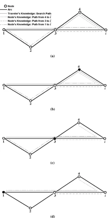
The following example illustrates the traveler-node learning rule graphically. In the example, all arc costs are assumed to be 1 for sim-plicity. A traveler originating from Node 1 just moved to node i (Figure 1a). Therefore, the traveler-node learning rule is applied between these two agents. In this case the traveler has already visited three nodes (n=3, i′ ∈{1, 3, 4}) before arriving at i. The traveler’s knowledge is represented in the diagram by the solid line, and the node’s knowledge is depicted by three types of discontinuous lines. The traveler and the node first compare the paths from Node 4 to i because Node 4 is the one most recently visited by the traveler. Since they know two equally short paths (1node=1traveler), there is no learn-ing activity between them (Figure 1b shows their respective knowl-edge after this comparison). Then they compare the two paths from Node 3 to i and find that the node knows a better path (1node< 2traveler). Thereby the traveler learns from the node (see Figure 1c after this
round of learning). Finally, they compare paths between the trav-eler’s origin Node 1 and node i. This time, the node learns from the traveler because the traveler knows a shorter path (3node> 2traveler; see bottom diagram in Figure 1d ).
The result of this traveler-node learning rule and Equation 2 is that, once a traveler agent finds an activity, the path it used will also be the shortest path from its origin to the destination, based, on the traveler’s best knowledge. Node agents also possess the knowledge of shortest paths identified by the model. If there are enough travel-ers in the transportation system, the shortest path found by the model approximates the real shortest paths, as will be seen in two exam-ples presented later. In this sense, the learning rule in this model could be viewed as an asymptotic shortest-path algorithm based on distributed learning.
Transportation planners are familiar with the application of discrete choice analysis in travel forecasting (3). Individuals’ route selection behavior is modeled as the outcome of a cross-sectional choice pro-cess that contains two steps: choice-set generation, in which several alternative routes are identified, and choice-making, in which a “best” route is selected on the basis of utility trade-offs. The learning rule just described is an example of another paradigm for modeling rout-ing decisions and can be interpreted as follows. A traveler agent is able to identify at least one route toward the activity destination (e.g., the traveler’s own search path); however, without any learn-ing activities with the nodes (holders of localized network informa-tion) along the traveler’s own search path, the selected route will be by no means satisfactory. The traveler agent also recognizes that fact and wants improvements. However, in contrast to discrete choice analysis, it is not assumed that travelers are capable of identifying several alternative routes. Rather, it is assumed that travelers adjust their current route on the basis of localized network information.
Such localized network information can come from other travel-ers or from traveltravel-ers’ own experience. When a traveler agent arrives at a node in the model and learns a better shortcut from the node agent, in the real world this situation can be interpreted as one in which someone tells someone else a better route. If alternatively the node agent learns from the traveler agent, the traveler agent actually shares its own experience to improve the collective understanding of the network. This phenomenon can also frequently be observed in the real world. For instance, a good route from a traveler’s home to the shopping center that is frequently visited by the traveler is very likely to become a part of the path selected by the same traveler for a trip from home to another destination near the shopping center.
The improvement or adaptation paradigm, in which travelers are assumed to adjust their decision until a certain aspiration level is achieved, was adopted in previous models of travel decision making, such as AMOS (22, 23) and SMASH (24). Bowman and Ben-Akiva (25) generalize the decision-making processes in those models as repetitive execution of choice-set generation and choice making. However, the intensive learning and adaptive behavior may be better modeled under an agent-based framework.
Emergence of Travel Demand Through Evolutionary Process
On the basis of the specified agent characteristics and interaction rules, a transportation system is ready to evolve given a transporta-tion network, an initial distributransporta-tion of travelers, and activity opportu-nities in the network, which can be the outputs of any trip generation process. The evolutionary process is illustrated by the flowchart in (a)
(b)
(c)
(d)
Figure 2. The probabilities specified in Equations 2 to 4 can be real-ized through Monte Carlo simulation. The convergence of the evolu-tion process can be directly measured by the number of residual travelers, that is, travelers who have not yet found an activity or the number of residual opportunities, whichever reaches zero first (the model does not require an equal number of travelers and opportuni-ties). When all travelers are settled with activities, the transportation system reaches a stable pattern since there will be no more move-ments or interactions. All agents and their knowledge will remain constant thereafter. Therefore, this stable pattern is considered the end point of the evolution or, for simplicity, an equilibrium.
If each traveler corresponds to one or more trips, the trip distribu-tion and assignment problems are solved simultaneously in the sys-tem equilibrium. The route each traveler takes is the shortest path from the origin to the destination based on the traveler’s best knowl-edge of the network travel costs. That knowlknowl-edge is accumulated through interactive, iterative learning with multiple node agents in the network. The result of route assignment in the agent-based travel demand model is in a sense similar to an all-or-nothing assignment since arc capacity constraints are not considered in the current model, although the two algorithms are based on completely different assumptions about travel behavior. The only coefficient that needs to be calibrated in the model is βin Equation 1, which can be interpreted as a traveler’s willingness to travel further.
APPLICATION EXAMPLES AND CALIBRATION PROCEDURES Computational Properties
Before the discussion proceeds to numerical examples, the compu-tational properties of the model are summarized analytically. For a transportation network with I nodes and T travelers, there are at most I*(I−1) +T paths in the model since each node can at most keep information on I−1 paths from all other nodes to itself, and each traveler has one search path. All knowledge must be stored in the model, and hence the theoretical maximum memory consumption is proportional to the number of travelers and the square of network size. In practice, the actual memory requirement is much less because if no traveler travels between a node pair, the shortest path between the two nodes is not necessary and will not be stored by any
node. In a large network, many node pairs will not be visited by trav-elers. As the system starts evolving, the number of paths further decreases since a traveler’s search path is no longer useful and can be deleted once an activity is found.
An examination of the evolutionary process (Figure 2) would reveal a good property of the model—the computational time is only proportional to the number of travelers and is not sensitive to the size of the transportation network. The running time of the model will still increase as the network size increases since on average travel-ers will search more nodes to find activities. The travel-node learn-ing process will take more time, but it will not increase exponentially because in the agent-based model, information exchange and agent learning activities substitute for standard shortest-path algorithms, and thus path enumeration is not required. Another aspect related to running time is the ease of the calibration procedure, which will be discussed next along with two examples.
Numerical Examples
Example 1: 10 ×10 Grid Network
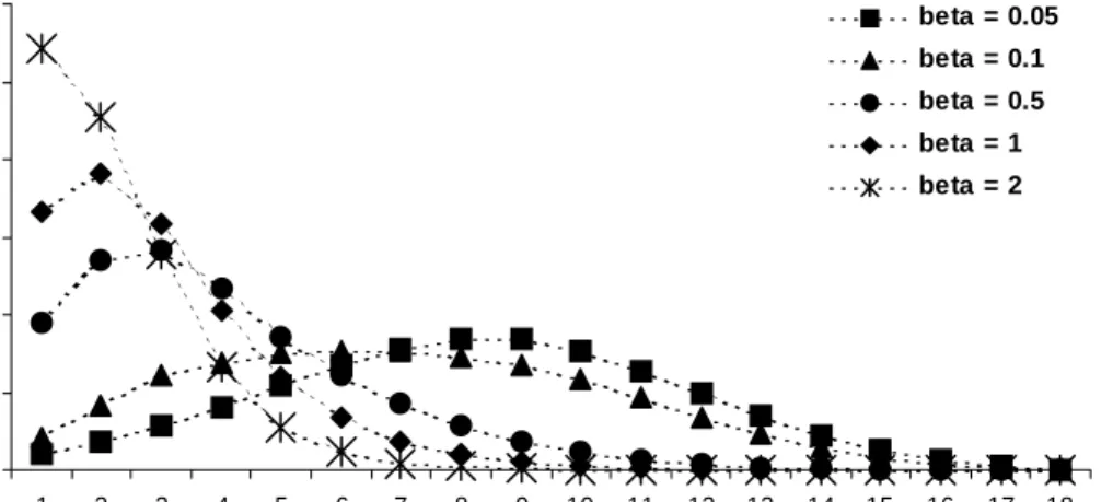
The first example uses a simple 10 ×10 grid network with 300,000 travelers and an equal number of opportunities to demonstrate the model. The travelers and opportunities are uniformly distributed among all nodes. The arc cost is 1 unit for all arcs (see Figure 3). The structure of the agent-based travel demand model can be im-plemented with any object-oriented programming language (Java was used in this study). Five different β’s are tested ranging from 0.05 to 2. For each β, the resulting travel length distributions and the convergence properties at the five equilibria are summarized in Figures 4 and 5, respectively.
The model can approximate a variety of trip length distributions with negative exponential (large β) and normal distribution (small β) at the two extremes. In this small network with a moderate number of travelers, the evolutionary process quickly reaches the equilib-rium. As travelers travel farther away from origins to find activity opportunities, it takes longer for the system to achieve the equilib-rium. In all five scenarios, at equilibrium the shortest paths identi-fied by the models are the real shortest paths between node pairs, which is not surprising in a small network. As the ratio of number of travelers to the size of the network decreases, some shortest paths learned by the travelers in the model may be longer than the real shortest paths, as will be seen in the next example. The selection of the initial random seed for Monte Carlo simulation has almost no impact on the resulting trip length distribution and shortest paths at the equilibrium, probably because the large number of random deci-sions and learning activities in the model tends to average out the initial variability due to different random seeds.
Example 2: Chicago, Illinois, Sketch Network and Model Calibration
In the second example, the agent-based travel demand model is applied to the Chicago sketch network, consisting of 933 nodes and 2,950 links, a fairly realistic yet aggregated representation of the Chicago region developed by the Chicago Area Transportation Study (CATS) (1). There are more than 1.26 million travelers in this test network accord-ing to the trip generation data, with each traveler representaccord-ing one trip. The only coefficient βin the model is calibrated against CATS 1990 Household Travel Survey (HTS) data. The estimated travel time
FIGURE 2 Flowchart of evolutionary algorithm.
YES NO NO YES NO YES YES NO Initialization
All traveler goals achieved? End Update node i Last node? Update traveler w Last traveler?
Update arc i-j
Last arc?
Collect statistics
Specify number of travelers and travel opportunities at each node; all traveler status = 0;
all node knowledge = none Get number of travel opportunities at demand nodes and update turning guidance matrix P If(status = 1), exit; else: determine next node; If(stay), status = 1; else: move to the next node; update searching path; apply traveler-node learning rule Update arc flow and cost Initialization
All traveler goals achieved? End Update node i Last node? Update traveler w Last traveler?
Update arc i-j
Last arc?
Collect statistics
Specify number of travelers and travel opportunities at each node; all traveler status = 0;
all node knowledge = none Get number of travel opportunities at demand nodes and update turning guidance matrix P If(status = 1), exit; else: determine next node; If(stay), status = 1; else: move to the next node; update searching path; apply traveler-node learning rule Update arc flow and cost
Node 1 3000 travelers 3000 opportunities Node 2 3000 travelers 3000 opportunities Arc 2-1 Arc 1-2 Node 1 3000 travelers 3000 opportunities Node 2 3000 travelers 3000 opportunities Arc 2-1 Arc 1-2 735 veh/lane/hr 0 20000 40000 60000 80000 100000 120000 1 2 3 4 5 6 7 8 9 10 11 12 13 14 15 16 17 18 Travel Costs Number of Trips beta = 0.05 beta = 0.1 beta = 0.5 beta = 1 beta = 2 0 50000 100000 150000 200000 250000 300000 350000 2 5 10 20 30 45 60 65
CPU Time (sec)
Residual Travelers beta = 0.05 beta = 0.1 beta = 0.5 beta = 1 beta = 2
FIGURE 4 Trip length distribution with various ’s for 10 10 grid network.
FIGURE 5 Convergence speeds with various ’s for 10 10 grid network.
FIGURE 3 Uniform distribution of travelers and opportunities for 10 10 grid network.
distribution with various β’s and the observed distribution are plotted in Figure 6. The spikes on the observed travel time distribution reveal survey participants’ tendencies to round their actual travel times to 30, 45, and 60 min. The mean square error (MSE) between the esti-mated and the observed distribution is plotted against βin Figure 7. It is clear in this graph that the MSE distribution is a unimodal one, and therefore simple one-dimensional search methods can be adopted to calibrate the model coefficient. The following is an applicable calibration procedure based on golden section search:
Step 0—Initialization: Lower-bound β−=0.1 and upper-bound
β+=1. (Theoretically, βcan be any positive value, but for all
prac-tical purposes, [0.1, 1] should be a safe starting interval for the golden section search.) Determine stopping tolerance e > 0. Itera-tion counter t=0. Compute β1= β+−0.618 (β+− β−) and β2= β−+ 0.618 (β+− β−). Evaluate the MSEs at all four points.
Step 1—Stopping: If (β+− β−) < e, stop, and the optimal β* =0.5
(β++ β−). Otherwise, proceed to Step 2.
Step 2—Iteration: If MSE (β1) < MSE (β2), narrow the search to the left part of the interval by updating β+= β2, β2= β1, β1= β+− 0.618 (β+− β−), and evaluate the new MSE (β1). If MSE (β1) > MSE (β2), narrow the search to the right part of the interval by
updating β−= β1, β1= β2, β2= β−+0.618 (β+− β−), and evaluate the new MSE (β2).
t=t+1. Return to Step 1. ϒ
Other one-dimensional search methods can be used as well, but the golden section search in general provides an efficient procedure. A more detailed discussion of unimodal function optimization may be found elsewhere (26 ). The foregoing calibration procedure was applied to the Chicago sketch network with e=0.05 and the optimal β* was found to be 0.42 after five golden section search iterations (i.e., six executions of the model with different β’s since the first iter-ation requires the evaluiter-ation of model MSEs twice), which took about 70 CPU minutes on a Pentium IV, 1.7-GHz personal computer. At the equilibrium with β*, travelers discovered 99.1% of all origin– destination paths, of which more than 98% are real shortest paths.
However, the β* estimated on one network is not directly trans-ferable to other networks. For instance, the coefficient estimated for a sketch network that only includes major highways should not be used without further calibration for a full network with all types of roads. One needs to be consistent in coding the network when apply-ing the proposed model. Of course, it is suspected that the coefficient also varies from city to city. From a computational point of view, the
0 100000 200000 300000 400000 500000 600000 5 10 15 20 25 30 35 40 45 50 55 60 65 70 75 80 85 90 >90
Trip Length (min)
Number of Trips Observed 1990 HTS Beta = 0.02 Beta = 0.1 Beta = 0.42 Optimum Beta = 1 Beta = 2 Iteration t = 0 t = 1 t = 2 t = 3 t = 4 t = 5 e < 0.05 ß * 1 3 5 7 9 11 0.02 0.05 0.1 0.15 0.2 0.25 0.3 0.35 0.42 0.45 0.5 0.55 0.6 1 2 beta MSE( β )/MSE(0.42) β
Intervals in the gold section search
FIGURE 6 Chicago sketch network: trip length distribution with various ’s.
model transferability is not a big issue because it does not take much time to calibrate βfor a specific network, but the estimated β’s for different urban areas are not comparable. The β-coefficient is sensi-tive to the detail of the network used for calibration because in the proposed model, travelers base their next movements only on the relative distribution of activity opportunities at surrounding nodes. To improve the transferability of the model, one needs to relate the probability that a traveler agent will accept an activity opportunity with the actual distance (or duration) of travel.
The agent-based model after the calibration procedure distributes trips from origins to destinations in a disaggregate manner with a trip length distribution reasonably close to the observed one and assigns most traffic to the shortest routes. The model provides output statis-tics including arc flows, the origin and destination of each individual trip, the path of each individual trip, and turning proportions at all intersections.
POSSIBLE EXTENSIONS OF MODEL AND FUTURE RESEARCH DIRECTIONS
Though the proposed agent-based travel demand model is a novel and interesting way of forecasting travel demand, it has not achieved the scope of existing travel forecasting methods. Several extensions can be incorporated to improve the current model.
More Agent Characteristics and Knowledge
With only three types of agents and minimum agent characteristics, the proposed agent-based travel demand model is able to accomplish two critical steps in the travel forecasting process—trip distribution and traffic assignment—within a short amount of time. It would be worthwhile to extend the basic model so that mode split can also be incorporated and more-realistic traffic assignment algorithms can be approximated. One way to enable modal split in the agent-based model is to expand the node knowledge to path costs of all modes and embed a mode choice rule into travelers’ characteristics. Con-gestion effects should be taken into account in future versions of the model, which requires an expansion of arc characteristics. However, with limited arc capacities, the shortest paths become dependent on travelers’ choices. How traveler agents learn shortest paths in this new dynamic situation must be carefully modeled, probably through repetitive information exchange and learning from day to day.
More Types of Agents
Besides travelers, nodes, and arcs, other agents in the transportation system have significant impacts on travel demand. For instance, it is necessary to define agents that represent transit links and railways if these modes are to be incorporated in the model. Another exten-sion of the current agent-based model would be the introduction of land use agents. The interaction between transportation and land use has been long recognized and studied. A metropolitan area can be divided into many land use cells, and each cell can be modeled as a special type of agent that has its own characteristics and behavioral rules. In an agent-based model, interaction rules between land use cells and transportation agents such as nodes and arcs, if appropri-ately defined, may be able to reasonably replicate the feedback between transportation and land use. The problem then becomes
the calibration of these rules. Also, under the agent-based modeling framework, simple rules may well explain complicated real-world phenomena such as the transportation–land use feedback loop. Alter-natively, urban land use can be modeled as the environment in the agent-based model. These possibilities should be examined in future studies. Transportation management policies, such as pricing schemes and financing strategies, have already been modeled by proper agents and their characteristics in several previous studies (27, 28).
More-Realistic Rules of Agent Behaviors
In constructing an agent-based model there are two major steps: (a) identify agents and their characteristics and (b) specify their behavioral rules. Different modelers may come up with different sets of agents for the same system. Some may be more useful in terms of facilitating the second step, rule specification, which is usu-ally the challenging part. The model developed in this study employs only local rules according to which agents interact only with other adjacent agents. Local rules have been successfully used in many cellular automata applications, such as the cell transmission model for freeway traffic (29, 30). In general, drivers make car-flowing and lane-changing decisions on the basis of the traffic conditions around themselves, and therefore local rules may be a realistic specification of their interactions. However, in the case of travel decision mak-ing, it is known that travelers sometimes rely on maps, media, and even route guidance systems when making decisions. This aspect implies that information sharing is beyond the local level.
Although occasionally global knowledge sharing, information flow, and learning activities can be reasonably approximated with local rules, that is not always the case. Do travelers find their activi-ties and choose routes using the same methodology in the proposed agent-based travel demand model? Will a small deviation from real behavior significantly affect the resulting equilibrium of the evolu-tionary process? These questions are yet to be answered. In the two examples given in the previous section, travelers have no difficulty in finding the shortest path for their trips because there are so many travelers in the system and the intensive local learning activities solve the shortest paths for travelers. Had there been only one traveler agent in the model, it would definitely fail to find the shortest paths since no learning activities would happen. But because a single traveler in the real world can identify the shortest route for a trip (or at least a route not much longer than the shortest one) without interacting with other individual travelers, global knowledge sharing may need to be incorporated somehow into the agent-based travel demand model.
The progress made in travel behavior studies can be readily incor-porated into the agent-based model with an update of agent behav-ioral rules. The only problem with more-realistic behavbehav-ioral rules is their possible requirements for more computational resources. Find-ing and applyFind-ing realistic behavioral rules of agents while at the same time keeping the model computationally feasible is the real chal-lenge. This challenge should be kept in mind in future development of similar models. Because the human brain has a limit on complex computation, this problem may not be as serious as it seems.
CONCLUSIONS
An agent-based travel demand model is developed. Travel demand emerges from the interactions of three types of agents in the trans-portation system: node, arc, and traveler. Simple local rules of agent
behaviors are shown to be capable of efficiently solving complex transportation problems such as trip distribution and route assign-ment. The model also provides an asymptotic shortest-path algorithm based on distributed agent learning activities. Possible extensions to the basic model are also discussed. The generic and flexible struc-ture of the agent-based modeling method makes it easier to develop new models and to expand existing models. By giving agents intel-ligence and allowing them to learn, modelers can accomplish more with less modeling effort. The method also takes full advantage of the fast-growing computational power now available.
Compared with trip-based approaches, activity-based approaches represent a new paradigm for travel demand analysis. The proposed agent-based technique, however, does not imply another paradigm shift. Rather, it is a powerful modeling tool to disentangle complex systems. In general, agent-based models emphasize, at the micro-scopic level, searching and learning behavior, agents’ perception of the environment, information flow, interagent interactions, and heuristics and, at the macroscopic level, self-organization, hierar-chy, and other evolutionary properties. It is difficult and unneces-sary to draw a line between agent-based travel demand models and activity-based approaches. The modeling needs for interpersonal linkages, person–environment interactions, and longitudinal aspects of travel behavior discovered in recent practice of activity-based travel analysis actually provide a stage for agent-based modeling techniques. Some recent activity-based microsimulation studies in which learning behavior (31) and activity interactions (32) are explicitly modeled have demonstrated the increasing popularity of agent-based methods.
This study pushes the application of agent-based methods for travel analysis beyond the scope of origin–destination demand estimation and into the realm of traffic assignment. It is possible that even the traditional equilibrium assignment process could be replaced with an agent-based model. A completely agent-based travel forecasting system is worth pursuing in the future. Though the proposed model is rudimentary in its current form, the authors hope that it can attract more research interest in applying agent-based modeling techniques to travel forecasting.
ACKNOWLEDGMENTS
The authors thank David Boyce and Hillel Bar-Gera for their provi-sion of the Chicago sketch network and related transportation plan-ning data. Several smaller transportation networks on Bar-Gera’s Traffic Assignment Problem website (www.bgu.ac.il/∼bargera/tntp) were used in an earlier stage of the study.
REFERENCES
1. State of Illinois, Cook County, and City of Chicago. Chicago Area Trans-portation Study: Final Report. Bureau of Public Roads, U.S. Department of Commerce, 1959–1962.
2. Beckman, M., C. B. McGuire, and C. B. Winsten. Studies in the Eco-nomics of Transportation. Yale University Press, New Haven, Conn., 1956.
3. Ben-Akiva, M., and S. R. Lerman. Discrete Choice Analysis: Theory and Application to Travel Demand. MIT Press, Cambridge, Mass., 1985. 4. Recker, W. W., M. G. McNally, and G. S. Root. A Model of Complex
Travel Behavior, Part I: Theoretical Development. Transportation Re-search, Vol. 20A, 1986, pp. 307–318.
5. Recker, W. W., M. G. McNally, and G. S. Root. A Model of Complex Travel Behavior, Part II: Operational Model. Transportation Research, Vol. 20A, 1986, pp. 319–330.
6. Kitamura, R., E. I. Pas, C. V. Lula, K. Lawton, and P. E. Benson. The Sequenced Activity Mobility Simulator (SAMS): An Integrated Approach to Modeling Transportation, Land Use and Air Quality. Transportation, Vol. 23, 1996, pp. 267–291.
7. Ortuzar, J. D., and L. G. Willumsen. Modelling Transport, 3rd ed. Wiley, New York, 2001.
8. Boyce, D. Is the Sequential Travel Forecasting Paradigm Counterpro-ductive? Journal of Urban Planning and Development, ASCE, Vol. 128, No. 4, 2002, pp. 169–183.
9. Pas, E. I. State of the Art and Research Opportunities in Travel Demand: Another Perspective. Transportation Research, Vol. 21A, 1985, pp. 431–438.
10. Carpenter, S., and P. Jones, eds. Recent Advances in Travel Demand Analysis. Gower, Aldershot, England, 1983.
11. Jones, P., ed. Developments in Dynamic and Activity-Based Approaches to Travel Analysis. Avebury, Brookfield, Vt., 1990.
12. Kitamura, R. An Evaluation of Activity-Based Travel Analysis. Trans-portation, Vol. 15, 1988, pp. 9–34.
13. Ettema, D., and H. Timmermans, eds. Activity-Based Approaches to Travel Analysis. Pergamon Press, Oxford, United Kingdom, 1997. 14. McNally, M. G., and W. W. Recker. Activity-Based Models of Travel
Behavior: Evolution and Implementation. Elsevier Science, Amsterdam, Netherlands, 2000.
15. Von Neumann, J. Theory of Self-Reproducing Automata (A. W. Burk, ed.), University of Illinois Press, Urbana, 1966.
16. Intelligent Agents in Traffic and Transportation (special issue). Trans-portation Research, Vol. 10C, 2002, pp. 325–527.
17. Stouffer, S. A. Intervening Opportunities: A Theory Relating Mobility and Distance. American Sociological Review, Vol. 5, 1940, pp. 845–867. 18. Schneider, M. Gravity Models and Trip Distribution Theory. Papers of
the Regional Science Association, Vol. 5, 1959, pp. 51–56.
19. Haynes, K. E., and A. S. Fotheringham. The Gravity Model and Spatial Interaction. Sage Publications, Beverly Hills, Calif., 1984.
20. Benshoof, J. A. Characteristics of Drivers’ Route Selection Behavior. Traffic Engineering and Control, Vol. 11, No. 12, 1970, pp. 604–610. 21. Bovy, P. H. L., and E. Stern. Route Choice: Wayfinding in Transport
Networks. Kluwer Academic Publishers, Dordrecht, Netherlands, 1990, 56 pp.
22. Kitamura, R., C. V. Lula, and E. I. Pas. AMOS: An Activity-Based, Flexible and Truly Behavioral Tool for Evaluation of TDM Measures. Proceedings of Seminar D, 21st PTRC Summer Annual Meeting, PTRC Education and Research Service, Ltd., London, 1993, pp. 283–294. 23. RDC, Inc. Activity-Based Modeling System for Travel Demand
Fore-casting. U.S. Department of Transportation; Environmental Protection Agency, 1995.
24. Ettema, D., A. Borgers, and H. Timmermans. Simulation Model of Activity Scheduling Behavior. In Transportation Research Record 1413, TRB, National Research Council, Washington, D.C., 1993, pp. 1–11. 25. Bowman, J. L., and M. E. Ben-Akiva. Activity-Based Travel
Fore-casting. In Activity-Based Travel Forecasting Conference, June 2–5, 1996: Summary, Recommendations and Compendium of Papers, Report DOT-T-97-17, U.S. Department of Transportation, 1997. 26. Rardin, R. L. Optimization in Operations Research. Prentice Hall, Upper
Saddle River, N.J., 1998.
27. Yerra, B., and D. M. Levinson. The Emergence of Hierarchy in Trans-portation Networks. Presented at Western Regional Science Association Meeting, Rio Rico, Ariz., 2003.
28. Zhang, L., and D. Levinson. A Model of the Rise and Fall of Roads. Pre-sented at 50th North American Regional Science Council Annual Meet-ing, Philadelphia, Pa., Nov. 2003.
29. Daganzo, C. F. The Cell Transmission Model: A Dynamic Representa-tion of Highway Traffic Consistent with the Hydrodynamic Theory. Transportation Research, Vol. 28B, No. 4, 1994, pp. 269–287. 30. Daganzo, C. F. The Cell Transmission Model, Part II: Network Traffic.
Transportation Research, Vol. 29B, No. 2, 1995, pp. 79–93. 31. Arentze, T., and H. Timmermans. ALBATROSS: A Learning-Based
Transportation Oriented Simulation System. Eindhoven University of Technology, Netherlands, 2000.
32. Rindt, C. R., J. E. Marca, and M. G. McNally. An Agent-Based Activity Microsimulation Kernel Using a Negotiation Metaphor. Paper UCI-ITS-AS-WP-02-7. Center for Activity Systems Analysis, University of California, Irvine, 2002.
Publication of this paper sponsored by Passenger Travel Demand Forecasting Committee.