Numerical resolution of an exact heat conduction model with a delay term

(1)

UPCommons

Portal del coneixement obert de la UPC

http://upcommons.upc.edu/e-prints

Initially published in

Journal of Applied Analysis and Computation

.

The final authenticated version is available online at:

http://dx.doi.org/10.11948/2019.332

.

Published paper

:

Campo, M.; Fernández, J.; Quintanilla, R. Numerical resolution of an

exact heat conduction model with a delay term. "Journal of applied

analysis and computation", Febrer 2019, vol. 9, núm. 1, p. 332-344.

doi:

10.11948/2019.332

URL d'aquest document a UPCommons E-prints:

(2)

Volume 9, Number 1, February 2019, 332–344 DOI:10.11948/2019.332

NUMERICAL RESOLUTION OF AN EXACT

HEAT CONDUCTION MODEL WITH A DELAY

TERM

∗

Marco Campo

1

_{, José R. Fernández}

2,†

_{and Ramón Quintanilla}

3

Abstract In this paper we analyze, from the numerical point of view, a dynamic thermoelastic problem. Here, the so-called exact heat conduction model with a delay term is used to obtain the heat evolution. Thus, the ther-momechanical problem is written as a coupled system of partial differential equations, and its variational formulation leads to a system written in terms of the velocity and the temperature fields. An existence and uniqueness result is recalled. Then, fully discrete approximations are introduced by using the clas-sical finite element method to approximate the spatial variable and the implicit Euler scheme to discretize the time derivatives. A priori error estimates are proved, from which the linear convergence of the algorithm could be derived under suitable additional regularity conditions. Finally, a two-dimensional numerical example is solved to show the accuracy of the approximation and the decay of the discrete energy.

Keywords Thermoelasticity, exact heat condution, delay parameter, finite elements, a priori error estimates.

MSC(2010) 74K10, 35G50, 37N15, 74F05, 65M60, 65M12.

1. Introduction

The classical linear theory of heat conduction, based on Fourier’s law, implies that thermal perturbations will be felt instantly at all the points of the body. That is, the thermal waves propagate with infinity speed. It is physically unrealistic because of causality’s fundamental role in modern physics. Different heat conduction theories have been put forth over the course of the 20th century and the present century (see Chandrasekharaiah [2], Hetnarski and Ignaczak [10,11] and the references cited therein). In the books [12,26], several studies concerning applicability of nonclassical thermoelastic theories are considered.

†_{the corresponding author. Email address: [email protected](J.R.} Fer-nández)

1_{Departamento de Matemáticas, ETS de Ingenieros de Caminos, Canales y}

Puertos, Universidade da Coruña, Campus de Elviña, 15071 A Coruña, Spain

2_{Departamento de Matemática Aplicada I, Universidade de Vigo, ETSI}

Tele-comunicación, Campus As Lagoas Marcosende s/n, 36310 Vigo, Spain

3_{Departamento de Matemáticas, E.S.E.I.A.A.T.-U.P.C., Colom 11, 08222}

Ter-rassa, Barcelona, Spain

∗_{The work of M. Campo and J. R. Fernández has been supported by the} Min-isterio de Economía y Competitividad under the research project MTM2015-66640-P (with the participation of FEDER). The work of R. Quintanilla has been supported by the Ministerio de Economía y Competitividad under the research project MTM2016-74934-P (AEI/FEDER, UE).

(3)

In 1995, Tzou [24,25] suggested a theory where the heat flux and the gradient of the temperature have a delay in the constitutive equations. The constitutive equations proposed by Tzou are given by

qi(x, t+τ1) =−κθ,i(x, t+τ2), κ >0, (1.1)

where τ1 and τ2 are the delay parameters which are assumed to be positive.This

equation says that the temperature gradient established across a material volume at position x and time t+τ2 results in a heat flux to flow at a different time

t+τ1. The delays can be understood in terms of the microstructure of the material.

This theory has several derivations when the heat flux and the gradients of the temperature and the thermal displacement are replaced by Taylor approximations. More recently, Choudhuri [3] proposed a constitutive law with three-phase-lag which is an extension of Tzou’s proposition. The equation is

qi(x, t+τ1) =−k1α,i(x, t+τ3)−k2θ,i(x, t+τ2), (1.2)

where α˙ = θ. The variable α is called the thermal displacement. The parameter

τ3 is another delay parameter. It seems that the aim of Choudhuri was to

estab-lish a mathematical model that includes phase-lags in the heat flux vector, in the temperature gradient and in the thermal displacement gradient. Moreover, if Tay-lor approximation is introduced in the equation, the Green and Naghdi models are obtained [7,8].

These two proposals lead toill-posedproblems in the sense of Hadamard. In fact, it can be shown that combining equation (1.1) (or (1.2)) with the energy equation

cθ˙+ div q= 0, (c >0), (1.3) leads to the existence of a family of elements in the point spectrum such that its real part tends to infinity [5]. It has been also showed that the Tzou’s theory is not compatible with the basic axioms of the thermomechanics [6]. Therefore, it is difficult to accept these proposals either from a mathematical point of view or from the thermodynamical perspective.

In a recent note [21] it was proved that when τ3 < τ1 = τ2, equation (1.2)

combined with the energy equation (1.3) defines a well posed problem. That is, a well posed problem in the context of the exact three-dual-phase theory. This was a non-trivial case with this property. We could accept it as a possible exact phase-lag constitutive equation to describe the heat conduction which is different from the ones proposed in [19,20].

As it was used in the theories proposed by Choudhuri and Tzou, we could replace equation (1.2) by truncated Taylor expansions. If we consider a second order approximation we find the heat equation:

¨ ν−k

∗_τ2

2 ∆¨ν = (k1+k

∗_τ_)∆θ₊_k∗_∆ν,

where now we assume thatτ =τ3−τ1(=τ2)>0. This heat conduction equation

has been complemented with other equations to obtain a thermoelastic problem and several contributions has been dedicated to study it. We recall some of them [13–18,22].

(4)

2. The mechanical and variational problems:

exis-tence and uniqueness

In this section, we present a brief description of the model and we obtain its me-chanical and variational formulations (details can be found in [22]). We also recall an existence and uniqueness result.

Let Ω⊂Rd_, _d_{= 1,}_2,₃_{, be the domain and denote by} _{[0, T}_]_, _{T >} ₀_{, the time}

interval of interest. The boundary of the bodyΓ =∂Ωis assumed to be Lipschitz. Moreover, let x∈Ωand t∈[0, T] be the spatial and time variables, respectively. In order to simplify the writing, we do not indicate the dependence of the functions onx= (xj)dj=1andt, and a subscript after a comma under a variable represents its

spatial derivative with respect to the prescribed variable, i.e. fi,j =

∂fi

∂xj

. The time derivatives are represented as a dot for the first order and two points for the second order over each variable. Finally, as usual the repeated index notation is used for the summation.

We denote by u = (ui)di=1 and ν the displacement field and the thermal

dis-placement, respectively. We note that the temperatureθis then obtained asθ= ˙ν. Assuming that the material is isotropic and homogeneous and following the work by Quintanilla [22], the model is written as follows, fori, j= 1, . . . , d, inΩ×(0, T),

ρ¨ui−µui,jj−(λ+µ)uj,ji−βθ,i= 0,

cν¨−τ 2 2 k ∗_∆¨_ν ₌_β_u_˙ i,i+k∗∆ν+ (k1+τ k∗)∆ ˙ν. (2.1)

In the above equations, constantsρandk∗denote the mass density and the thermal diffusion coefficient, respectively, and λ and µ represent the Lamé’s coefficients. Moreover,β is a thermal expansion coefficient andτ is the delay parameter.

As boundary conditions, we assume, fori= 1, . . . , d,

ui(x, t) =θ(x, t) = 0 for(x, t)∈∂Ω×(0, T). (2.2)

We point out that other boundary conditions could be used but we restrict ourselves to this case for the sake of simplicity.

In order to complete the definition of the mechanical problem we impose the following initial conditions forx∈Ω:

ui(x,0) =u0i(x), u˙i(x,0) =vi0(x), ν(x,0) =ν 0₍_x_), ˙ ν(x,0) =θ0(x), (2.3) whereu0_{= (u}0

i)di=1,v0= (v0i)di=1,ν0 andθ0 are prescribed functions.

Therefore, the thermo-mechanical problem modelling the deformation of a ther-moelastic body with an exact heat conduction model with a delay is the following (see [22] for details).

Problem P.Find the displacement fieldu= (ui)di=1: Ω×[0, T]→Rdand the

ther-mal displacementν: Ω×[0, T]→Rsuch that equations (2.1), boundary conditions (2.2) and initial conditions (2.3) are fulfilled.

Now, in order to obtain the variational formulation of Problem P, letY =L2(Ω),

(5)

respective scalar products in these spaces, with corresponding norms∥ · ∥Y,∥ · ∥H

and∥ · ∥Q. Moreover, let us define the variational spacesV andE as follows,

V ={z∈[H1_(Ω)]d_;_z₌₀ _on _Γ_}_,

E={r∈H1_{(Ω) ;}_r_{= 0} _on _Γ_}_,

with respective scalar products(·,·)V and(·,·)E, and norms∥ · ∥V and∥ · ∥E.

By using Green’s formula and boundary conditions (2.2), we write the variational formulation of Problem P in terms of the velocity fieldv= ˙uand the temperature

θ= ˙ν.

Problem VP.Find the velocity fieldv: [0, T]→V and the temperatureθ: [0, T]→

Esuch thatv(0) =v0_,_{θ(0) =}_θ0_,_{and, for a.e.} _t_∈_{(0, T}₎_{and for all}_w_∈_V_,_r_∈_E_,

ρ( ˙v(t),w)H+ (λ+µ)(divu(t),divw)Y +µ(∇u(t),∇w)Q −β(∇θ(t),w)H= 0, (2.4) c( ˙θ(t), r)Y + τ2 2 k ∗₍_∇_θ(t),˙ _∇_r) H+k∗(∇ν(t),∇r)H +(k1+τ k∗)(∇θ(t),∇r)H=β(divv(t), r)Y, (2.5)

where the displacement field and the thermal displacement are then recovered from the relations u(t) = ∫ t 0 v(s)ds+u0, ν(t) = ∫ t 0 θ(s)ds+θ0, (2.6)

and we note thatdiv represents the classical divergence operator.

In [22] it has been proved the following existence and uniqueness result.

Theorem 2.1. Let the following conditions on the constitutive coefficients hold:

ρ >0, µ >0, λ >0, c >0, τ >0, k∗ >0, k1>0. If the initial conditions satisfy:

u0,v0∈V, ν0, θ0∈E,

then there exists a unique solution to Problem VP with the following regularity:

u∈C1([0, T];V)∩C2([0, T];H), ν∈C2([0, T];E).

3. Fully discrete approximations: an a priori error

analysis

In this section, we now consider a fully discrete approximation of Problem V P. This is done in two steps. First, we assume that the domain Ωis polyhedral and we denote byTh_{a regular triangulation in the sense of [}₄_{]. Thus, we construct the}

finite dimensional spacesVh⊂V andEh⊂E given by

Vh={wh∈[C(Ω)]d; wh_|_{T r} ∈[P1(T r)]d ∀T r∈ Th, wh=0 on Γ}, (3.1)

(6)

whereP1(T r)represents the space of polynomials of degree less or equal to one in

the elementT r, i.e. the finite element spacesVh_and_Eh_{are composed of continuous}

and piecewise affine functions. Here,h >0denotes the spatial discretization para-meter. Moreover, we assume that the discrete initial conditions, denoted by u0h_,

v0h,θ0h andν0h, are given by u0h₌_Ph

1u0, v0h=P1hv0, θ0h=P2hθ0, ν0h=P2hν0, (3.3)

where Ph

1 and P2h are the classical finite element interpolation operators over Vh

andEh_{, respectively (see, e.g., [}₄_]).

Secondly, we consider a partition of the time interval [0, T], denoted by 0 = t0 < t1 < · · · < tN = T. In this case, we use a uniform partition with step

size k =T /N and nodes tn =n k for n= 0,1, . . . , N. For a continuous function

z(t), we use the notation zn =z(tn)and, for the sequence {zn}Nn=0, we denote by

δzn= (zn−zn−1)/k its corresponding divided differences.

Therefore, using the backward Euler scheme, the fully discrete approximations are considered as follows.

Problem VPhk_. _{Find the discrete velocity}_vhk ₌_{_vhk

n }Nn=0⊂Vh and the discrete temperature θhk = {θnhk}Nn=0 ⊂ Eh such that vhk0 = v0h, θhk0 = θ0h, and, for

n= 1, . . . , N and for all wh_∈_Vh _and_rh_∈_Eh_,

ρ(δvhk_n ,wh)H+ (λ+µ)(divuhkn ,divw h₎ Y +µ(∇uhkn ,∇w h₎ Q −β(∇θhkn ,wh)H = 0, (3.4) c(δθhkn , rh)Y + τ2 2 k ∗₍_∇_δθhk n ,∇rh)H+k∗(∇νnhk,∇rh)H +(k1+τ k∗)(∇θhkn ,∇r h₎ H=β(divvhkn , r h₎ Y, (3.5)

where the discrete displacement field and the discrete thermal displacement are then recovered from the relations

uhk_n =k n ∑ j=1 vhk_j +u0h, νhk_n =k n ∑ j=1 θhk_j +ν0h. (3.6)

We note that the existence of a unique discrete solution to Problem V Phk is obtained in a straightforward way using the classical Lax-Milgram lemma.

Now, we will find some a priori error estimates on the numerical errorsvn−vhkn

andθn−θnhk. We have the following.

Theorem 3.1. Under the assumptions of Theorem 2.1, if we denote by(u,v, θ, ν)

the solution to Problem V P and by (uhk_,_vhk_{, θ}hk_{, ν}hk₎ _{the solution to Problem}

V Phk_{, then we have the following a priori error estimates, for all}_wh₌_{_wh j}Nj=0⊂ Vh _and_rh₌_{_rh j}Nj=0⊂Eh, max 0≤n≤N { ∥vn−vhkn ∥ 2 H+∥∇(un−uhkn )∥ 2 Q+∥div(un−uhkn )∥ 2 Y +∥θn−θnhk∥ 2 Y +∥∇(θn−θnhk)∥ 2 H+∥∇(νn−νnhk)∥ 2 H } ≤Ck N ∑ j=1 ( ∥v˙j−δvj∥H2 +∥vj−whj∥ 2 V +∥u˙j−δuj∥2V

(7)

+∥θ˙j−δθj∥2E+∥∇( ˙νj−δνj)∥2H+∥θj−rjh∥ 2 E ) +C max 0≤n≤N∥vn−w h n∥ 2 H+C max 0≤n≤N∥θn−r h n∥ 2 Y +C k N_∑₋1 j=1 ∥θj−rhj −(θj+1−rjh+1)∥ 2 Y +C k N∑−1 j=1 ∥vj−whj −(vj+1−whj+1)∥ 2 H+C ( ∥v0−v0h∥2_H +∥u0−u0h∥2V +∥θ0−θ0h∥2E+∥∇(ν0−ν0h)∥2H ) , (3.7)

whereC >0 is a positive constant which is independent of the discretization para-metershandk, but depending on the continuous solution, andδvj = (vj−vj₋1)/k,

δuj = (uj−uj₋1)/k,δθj = (θj−θj₋1)/k andδνj = (νj−νj₋1)/k.

Proof. First, we obtain some estimates for the velocity field. Then, we subtract

variational equation (2.4) at timet=tn for a test functionw=wh∈Vh⊂V and

discrete variational equation (3.4) to obtain, for allwh_∈_Vh_,

ρ( ˙vn−δvhkn ,w h₎ H+ (λ+µ)(div(un−uhkn ),divw h₎ Y +µ(∇(un−uhkn ),∇wh)Q−β(∇(θn−θnhk),wh)H= 0,

and so, we have, for allwh∈Vh,

ρ( ˙vn−δvhkn ,vn−vhkn )H+ (λ+µ)(div(un−uhkn ),div(vn−vhkn ))Y

+µ(∇(un−uhkn ),∇(vn−vhkn ))Q−β(∇(θn−θnhk),(vn−vhkn ))H

=ρ( ˙vn−δvhkn ,vn−wh)H+ (λ+µ)(div(un−uhkn ),div(vn−wh))Y

+µ(∇(un−uhkn ),∇(vn−wh))Q−β(∇(θn−θnhk),vn−wh)H = 0.

Taking into account that

( ˙vn−δvhkn ,vn−vhkn )H≥( ˙vn−δvn,vn−vhkn )H + 1 2k { ∥vn−vhkn ∥ 2 H− ∥vn₋1−vhkn−1∥ 2 H } , (div(un−uhkn ),div(vn−vhkn ))Y ≥(div(un−uhkn ),div( ˙un−δun))Y

+ 1 2k { ∥div(un−uhkn )∥2Y−∥div(un−1−uhkn₋1)∥2Y } , (∇(un−uhkn ),∇(vn−vhkn ))Q≥(∇(un−uhkn ),∇( ˙un−δun))Q + 1 2k { ∥∇(un−uhkn )∥ 2 Q−∥∇(un−1−uhkn₋1)∥ 2 Q } , −β(∇(θn−θnhk),vn−wh)H=β(θn−θnhk,div(vn−wh))Y,

(8)

allwh_∈_Vh_, ∗ ρ 2k { ∥vn−vhkn ∥ 2 H− ∥vn₋1−vhkn−1∥ 2 H } −β(∇(ξn−ξnhk),vn−vhkn )H +λ+µ 2k { ∥div(un−uhkn )∥ 2 Y − ∥div(un−1−uhkn−1)∥ 2 Y } +µ 2k { ∥∇(un−uhkn )∥ 2 Q− ∥∇(un−1−uhkn₋1)∥ 2 Q } ≤C ( ∥v˙n−δvn∥2H+∥vn−wh∥2V +∥∇(un−uhkn )∥ 2 Q+∥u˙n−δun∥2V +∥div(un−uhkn )∥ 2 Y +∥θn−θnhk∥ 2 Y +∥vn−vhkn ∥ 2 H +(δvn−δvhkn ,vn−wh)H ) .

Now, we obtain the error estimates on the temperature. Then, we subtract variational equation (2.5) at timet=tn for a test function r=rh ∈Eh⊂E and

discrete variational equation (3.5) to obtain, for allrh_∈_Eh_,

c( ˙θn−δθhkn , r h₎ Y + τ2 2 k ∗₍_∇_(δθ n−δθhkn ),∇r h₎ H +(k1+τ k∗)(∇(θn−θnhk),∇rh)H +k∗(∇(νn−νhkn ),∇rh)H =β(div(vn−vhkn ), rh)Y,

and so we have, for allrh_∈_Eh_,

c( ˙θn−δθhkn , θn−θhkn )Y +k∗(∇(νn−νnhk),∇(θn−θhkn ))H +τ 2 2 k ∗₍_∇_(δθ n−δθhkn ),∇(θn−θhkn ))H + (k1+τ k∗)(∇(θn−θnhk),∇(θn−θnhk))H −β(div(vn−vnhk), θn−θhkn )Y =c( ˙θn−δθhkn , θn−rh)Y +k∗(∇(νn−νnhk),∇(θn−rh))H +τ 2 2 k ∗₍_∇_(δθ n−δθhkn ),∇(θn−rh))H + (k1+τ k∗)(∇(θn−θnhk),∇(θn−rh))H −β(div(vn−vnhk), θn−rh)Y.

Keeping in mind that

( ˙θn−δθnhk, θn−θnhk)Y ≥( ˙θn−δθn, θn−θhkn )Y + 1 2k { ∥θn−θhkn ∥2Y − ∥θn−1−θhkn₋1∥2Y } , (∇( ˙θn−δθnhk),∇(θn−θnhk))H≥(∇( ˙θn−δθn),∇(θn−θhkn ))H + 1 2k { ∥∇(θn−θhkn )∥ 2 H− ∥∇(θn₋1−θhkn−1)∥ 2 H } , (∇(νn−νnhk),∇(θn−θnhk))H≥(∇(νn−νnhk),∇( ˙νn−δνn))H + 1 2k { ∥∇(νn−νnhk)∥2H− ∥∇(νn−1−νnhk₋1)∥2H } , −β(div(vn−vnhk), θn−θnhk)Y =β(vn−vhkn ,∇(θn−θhkn ))H,

(9)

using several times Cauchy-Schwarz and Young inequalities we find that, for all rh_∈_Eh_, 1 2k { ∥θn−θhkn ∥ 2 Y − ∥θn−1−θhkn−1∥ 2 Y } +β(vn−vhkn ,∇(θn−θnhk))H + 1 2k { ∥∇(θn−θhkn )∥ 2 H− ∥∇(θn₋1−θhkn−1)∥ 2 H } + 1 2k { ∥∇(νn−νnhk)∥ 2 H− ∥∇(νn₋1−νnhk−1)∥ 2 H } ≤C ( ∥_θ˙_n₋_δθ_n_∥2 E+∥θn−rh∥E2 +∥θn−θhkn ∥ 2 Y +∥∇(θn−θhkn )∥2H+∥∇( ˙νn−δνn)∥2H+∥vn−vhkn ∥2H +(δθn−δθhkn , θn−rh)Y +∥∇(νn−νnhk)∥ 2 H ) .

Combining now these estimates we find that

ρ 2k { ∥vn−vhkn ∥ 2 H− ∥vn−1−vhkn₋1∥ 2 H } +µ 2k { ∥∇(un−uhkn )∥ 2 Q− ∥∇(un−1−uhkn−1)∥ 2 Q } +λ+µ 2k { ∥div(un−uhkn )∥ 2 Y − ∥div(un₋1−uhkn−1)∥ 2 Y } +1 2k { ∥θn−θhkn ∥ 2 Y − ∥θn₋1−θhkn−1∥ 2 Y } +1 2k { ∥∇(θn−θhkn )∥ 2 H− ∥∇(θn₋1−θnhk−1)∥ 2 H } +1 2k { ∥∇(νn−νnhk)∥ 2 H− ∥∇(νn₋1−νnhk−1)∥ 2 H } ≤C ( ∥v˙n−δvn∥2H+∥vn−wh∥2V +∥∇(un−uhkn )∥ 2 Q +∥u˙n−δun∥2V +∥div(un−uhkn )∥ 2 Y +∥vn−vhkn ∥ 2 H +∥θ˙n−δθn∥2E+∥θn−rh∥2E+ (δvn−δvnhk,vn−wh)H +(δθn−δθhkn , θn−rh)Y +∥θn−θhkn ∥ 2 Y +∥∇(θn−θhkn )∥ 2 H +∥∇( ˙νn−δνn)∥H2 +∥∇(νn−νnhk)∥ 2 H ) .

Multiplying the previous estimates bykand summing up the resulting equation, using the estimates on the temperature fields given above we have

∥vn−vhkn ∥ 2 H+∥∇(un−uhkn )∥ 2 Q+∥div(un−uhkn )∥ 2 Y +∥θn−θnhk∥ 2 Y +∥∇(θn−θnhk)∥ 2 H+∥∇(νn−νnhk)∥ 2 H ≤Ck n ∑ j=1 ( ∥v˙j−δvj∥H2 +∥vj−whj∥ 2 V +∥∇(uj−uhkj )∥ 2 Q +∥u˙j−δuj∥2V +∥div(uj−uhkj )∥ 2 Y +∥vj−vhkj ∥ 2 H +∥θ˙j−δθj∥E2 +∥θj−rjh∥ 2 E+ (δvj−δvhkj ,vj−whj)H +(δθj−δθjhk, θj−rhj)Y +∥θj−θjhk∥2Y +∥∇( ˙νj−δνj)∥2H +∥∇(θj−θhkj )∥2H+∥∇(νj−νjhk)∥2H ) +C ( ∥v0−v0h∥2H +∥u0−u0h∥2_V +∥θ0−θ0h∥2_E+∥∇(ν0−ν0h)∥2_H ) .

(10)

Finally, taking into account that k n ∑ j=1 (δθj−δθjhk, θj−rhj)Y = (θn−θhkn , θn−rhn)Y + (θ0h−θ0, θ1−rh1)Y + n−1 ∑ j=1 (θj−θhkj , θj−rhj −(θj+1−rjh+1))Y, k n ∑ j=1 (δvj−δvhkj ,vj−whj)H = (vn−vhkn ,vn−whn)H+ (v0h−v0,v1−wh1)H + n−1 ∑ j=1 (vj−vhkj ,vj−wjh−(vj+1−whj+1))H,

using the above estimates and a discrete version of Gronwall’s inequality (see [1]) we conclude the proof.

Remark 3.1. We note that error estimates (3.7) are the basis to get the

con-vergence order of the approximations given by Problem VPhk_{. Therefore, as an}

example, under the following additional regularity condition: u∈C1_{([0, T}_{]; [H}2_(Ω)]d₎_∩_H3_{(0, T}_;_H₎_∩_H2_{(0, T}_;_V_),

ν∈C1_{([0, T}_];_H2_(Ω))_∩_H3_{(0, T}_;_Y_),

using the classical results on the approximation by finite elements and the regulari-ties of the initial conditions (see, for instance, [4]), it follows that the approximations obtained by Problem VPhk _{are linearly convergent.}

4. Numerical results

In this final section, we describe the numerical scheme implemented in the well-known finite element code FreeFem++ for solving Problem VPhk_{(see [}₉_{] for details),}

and we show a numerical example to demonstrate the accuracy of the approxima-tions and the decay of the discrete energy.

4.1. Numerical scheme

Given the solution uhk

n−1,vhkn−1, θnhk−1 and νnhk−1 at time tn₋1, the velocity and the

temperature are obtained by solving the following discrete nonsymmetric linear system, for allwh∈Vh andrh∈Eh,

ρ(vhkn ,wh)H+k2(λ+µ)(divvhkn ,divwh)Y +k2µ(∇vhk_n ,∇wh)Q−kβ(∇θhkn ,w h₎ H =ρ(vhk_n₋₁,wh)H−k(λ+µ)(divuhkn₋1,divw h₎ Y −kµ(∇uhk_n₋₁,∇wh)Q+k(Hn,wh)H, c(θ_nhk, rh)Y + τ2 2 k ∗₍_∇_θhk n ,∇r h₎ H+k2k∗(∇θhkn ,∇r h₎ H +k(k1+τ k∗)(∇θhkn ,∇rh)H−β(divvhkn , rh)Y

(11)

=c(θ_nhk₋₁, rh)Y + τ2 2 k ∗₍_∇_θhk n−1,∇r h₎ H−kk∗(∇νhkn−1,∇r h₎ H +k(Pn, rh)Y,

where the discrete displacements and the discrete thermal displacement are then recovered from the relations

uhk_n =kvhk_n +uhk_n₋₁, ν_nhk=kθ_nhk+ν_nhk₋₁.

Here, for the sake of generality we added body forcesH and a heat supplyP.

4.2. Numerical example: convergence and energy decay

We will consider the following academic problem:

Problem Pex_. _{Find the displacements} _u _{: [0,}_1]_×_[0,_1]_×_[0,_1] _→ _R2 _{and the}

temperature θ: [0,1]×[0,1]×[0,1]→Rsuch that

¨ ui−ui,jj−2uj,ji−θ,i=Hi in[0,1]×[0,1]×[0,1], ˙ θ−1 2 ˙

θ,ii−2θ,ii−ν,ii−βu˙i,i=P in [0,1]×[0,1]×[0,1],

ui(x, y, t) =θ(x, y, t) = 0 for i= 1,2

and(x, y, t)∈∂([0,1]×[0,1])×[0,1], ui(x, y,0) = (xy(1−x)(1−y), xy(1−x)(1−y))

for (x, y)∈[0,1]×[0,1], ˙

ui(x, y,0) = (xy(1−x)(1−y), xy(1−x)(1−y))

for (x, y)∈[0,1]×[0,1],

θ(x, y,0) =xy(1−x)(1−y) for (x, y)∈[0,1]×[0,1], ν(x, y,0) =xy(1−x)(1−y) for (x, y)∈[0,1]×[0,1],

where the body forcesH and the heat supplyP are given by

H(x, y, t) =et_(x2_y2₋_x2_y₋_2x2₋_3xy2₋_5xy_{+ 6x}₋_5y2_{+ 9y}₋_2,

x2_y2₋_3x2_y₋_5x2₋_xy2₋_5xy_{+ 9x}₋_2y2_{+ 6y}₋_2),

P(x, y, t) =et(_x2_y2₋_3x2_y₋_2x2₋_3xy2_{+ 5xy}_{+ 2x}₋_2y2_{+ 2y})_.

We note that Problem Pex _{corresponds to Problem}_P _{with the following data:}

Ω = (0,1)×(0,1), T = 1, ρ= 1, µ=λ= 1, β = 1, τ = 1, c=k∗=k1= 1,

and the initial conditions, for(x, y)∈(0,1)×(0,1),

u0_{(x, y) =}_v0_{(x, y) = (xy(1}₋_x)(1₋_{y), xy(1}₋_x)(1₋_y))_,

(12)

Table 1. Numerical errors (×10) for somendandk. nd↓k→ 0.02 0.01 0.005 0.001 16 0.125254 0.088769 0.076804 0.082744 32 0.080294 0.045405 0.028722 0.019348 64 0.070355 0.035439 0.018915 0.006389 128 0.070268 0.033910 0.016746 0.003876 256 0.070462 0.034058 0.016683 0.003329

The exact solution to Problem Pex _{is the following one, for} _{(x, y, t)}_∈ _[0,_1]_×

[0,1]×[0,1]andi= 1,2,

ui(x, y, t) =θ(x, y, t) =xy(1−x)(1−y)et.

Our aim here is to show the numerical convergence of the finite element scheme. Therefore, several uniform partitions for the time interval and the domain, dividing

Ω = [0,1]×[0,1]into2(nd)2 _{triangles, have been performed. Note that the number}

of degrees of freedom is3(nd+ 1)2_.

In Table 1 the numerical errors given by

max 0≤n≤N { ∥vn−vhkn ∥ 2 H+∥∇(un−uhkn )∥ 2 Q+∥div(un−uhkn )∥ 2 Y +∥θn−θnhk∥ 2 Y +∥∇(θn−θnhk)∥ 2 H+∥∇(νn−νnhk)∥ 2 H } ,

and obtained for some discretization parameters nd and k, are shown, and the convergence of the numerical scheme clearly observed. The evolution of the error with respect to the parameterh+k is plotted in Figure 1.

0 0.02 0.04 0.06 0.08 0.1 0.12 h+k 0 0.002 0.004 0.006 0.008 0.01 0.012 0.014 E hk Asymptotic behaviour

Figure 1. Asymptotic behaviour of the numerical scheme.

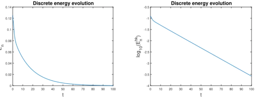
If we assume now that there are not volume forces, and we use the final time

T = 100s, and the same data and initial conditions than in the previous simulations, taking the discretization parametersh= 0.01andk= 0.001, the evolution in time

(13)

of the discrete energyEhk n , defined by (see [22]) Ehk n =ρ∥vhkn ∥H2 +µ∥∇uhkn ∥2Q+ (λ+µ)∥divuhkn ∥Y2 +c∥θhkn ∥2Y +τ 2 2 k ∗_∥∇_θhk n ∥ 2 H+k∗∥∇ν hk n ∥ 2 H

is plotted in Figure 2 in both natural and semi-log scales. We observe that an exponential energy decay has been achieved. Anyway, we note that in [22] it has been proved that such behaviour is not found in the continuous case.

0 10 20 30 40 50 60 70 80 90 100 t 0 0.02 0.04 0.06 0.08 0.1 0.12 0.14 En hk

Discrete energy evolution

0 10 20 30 40 50 60 70 80 90 100 t -4 -3.5 -3 -2.5 -2 -1.5 -1 -0.5 log 10 (E n hk )

Discrete energy evolution

Figure 2. Discrete energy evolution in natural and semi-log scales.

Acknowledgements.The authors are grateful to the anonymous referees for their

useful suggestions which improve the contents of this article.

References

[1] M. Campo, J. R. Fernández, K. L. Kuttler, M. Shillor and J. M. Viaño, Nu-merical analysis and simulations of a dynamic frictionless contact problem with damage, Comput. Methods Appl. Mech. Engrg., 2006, 196(1–3), 476–488. [2] D. Chandrasekharaiah, Hyperbolic thermoelasticity: A review of recent

litera-ture, ASME. Appl. Mech. Rev., 1998, 51(12), 705-?29.

[3] S. K. R. Choudhuri, On a thermoelastic three-phase-lag model, J. Thermal Stresses, 2007, 30, 231–238.

[4] P. G. Ciarlet, Basic error estimates for elliptic problems. In: Handbook of Numerical Analysis, P.G. Ciarlet and J.L. Lions eds., 1993, vol I, 17–351. [5] M. Dreher, R. Quintanilla and R. Racke,Ill-posed problems in

thermomechan-ics, Appl. Math. Letters, 2009, 22, 1374–1379.

[6] M. Fabrizio and F. Franchi, Delayed thermal models: stability and thermody-namics, J. Thermal Stresses, 2014, 37, 160–173.

[7] A. E. Green and P. M. Naghdi,On undamped heat waves in an elastic solid, J. Thermal Stresses, 1992, 15, 253–264.

[8] A. E. Green and P. M. Naghdi,Thermoelasticity without energy dissipation, J. Elasticity, 1993, 31, 189–208.

(14)

[9] F. Hecht, New development in FreeFem++, J. Numer. Math., 2012, 20(3–4), 251–265.

[10] R. B. Hetnarski and J. Ignaczak, Generalized thermoelasticity, J. Thermal Stresses, 1999, 22, 451–470.

[11] R. B. Hetnarski and J. Ignaczak,Nonclassical dynamical thermoelasticity, Int. J. Solids Struct. 2000, 37, 215–224.

[12] J. Ignaczak and M. Ostoja-Starzewski, Thermoelasticity with Finite Wave Speeds, Oxford Mathematical Monographs, Oxford, 2010.

[13] S. Kant, M. Gupta, O. N. Shivay and S. Mukhopadhyay,An investigation on a two-dimensional problem of Mode-I crack in a thermoelastic medium, Z. Ang. Math. Phys., 2018, 69, 21.

[14] A. Kumar and S. Mukhopadhyay, Investigation on the effects of temperature dependency of material parameters on a thermoelastic loading problem, Z. Ang. Math. Phys., 2017, 68, 98.

[15] B. Kumari, A. Kumar and S. Mukhopadhyay,Investigation of harmonic plane waves: detailed analysis of recent thermoplastic model with single delay term, Math. Mech. Solids, 2018. DOI: 10.1177/1081286518755232.

[16] B. Kumari and S. Mukhopadhyay,Fundamental solutions of thermoelasticity with a recent heat conduction model with a single delay term, J. Thermal Stresses, 2017, 40, 866–878.

[17] B. Kumari, and S. Mukhopadhyay, Some theorems on linear theory of ther-moelasticity for an anisotropic medium under an exact heat conduction model with a delay, Math. Mech. Solids, 2017, 22, 1177–1189.

[18] M. C. Leseduarte and R. Quintanilla, Phragmen-Lindelof alternative for an exact heat conduction equation with delay, Comm. Pure Appl. Anal., 2013, 12, 1221–1235.

[19] R. Quintanilla,A well-posed problem for the Dual-Phase-Lag heat conduction, J. Thermal Stresses, 2008, 31, 260–269.

[20] R. Quintanilla,A well-posed problem for the Three-Dual-Phase-Lag heat con-duction, J. Thermal Stresses, 2009, 32, 1270–1278.

[21] R. Quintanilla,Some solutions for a family of exact phase-lag heat conduction problems, Mech. Res. Commun., 2011, 38, 355–360.

[22] R. Quintanilla,On uniqueness and stability for a thermoelastic theory, Math. Mech. Solids, 2017, 22(6), 1387–396.

[23] O. N. Shivay and S. Mukhopadhyay,Some basic theorems on a recent model of linear thermoelasticity for a homogeneous and isotropic medium, Math. Mech. Solids, 2018. DOI: 10.1177/1081286518762612.

[24] D. Y. Tzou,A unified approach for heat conduction from macro to micro-scales, ASME J. Heat Transfer, 1995, 117, 8–16.

[25] D. Y. Tzou,The generalized lagging response in small-scale and high-rate heat-ing, Int. J. Heat Mass Transfer, 1995, 38, 3231–3240.

[26] L. Wang, X. Zhou and X. Wei, Heat Conduction: Mathematical Models and