Crude Oil Price
Differentials
An empirical analysis on th
e factors behind the
price
divergence
between
WTI and Brent
Martin Heier and Sindre Skoglund
Supervisor: Linda Nøstbakken
Master Thesis in Financial Economics
NORWEGIAN SCHOOL OF ECONOMICS
This thesis was written as a part of the Master of Science in Economics and Business Administration at NHH. Please note that neither the institution nor the examiners are responsible − through the approval of this thesis − for the theories and methods used, or results and conclusions drawn in this work.
Abstract
The main purpose of our thesis is to examine the long-run relationship between WTI and Brent. Historically, the prices fluctuated around a constant differential, where WTI traded above Brent due to its slightly higher quality. Recently, the differential has been reversed as Brent has traded at a premium to WTI since 2010. We analyze the unusual behavior in the price relationship with the use of an Engle-Granger two-step test for cointegration to assess if the relationship has ended, and whether a new has been formed. We also decompose the WTI-Brent spread to examine if the deviation can be accrued to supply or demand conditions. Finally, we build an empirical model to determine what factors have had a significant impact on the spread’s divergence.
We find that the long-run relationship between WTI and Brent ended in January 2010, and that a new relationship was established early 2014. However, the new relationship is different from its predecessor as Brent is now being traded at a premium to WTI. From our empirical findings we infer that insufficient pipeline infrastructure at Cushing is significant in explaining the spread’s divergence. We also conclude that shipping costs significantly affected the spread and have prolonged the divergence between WTI and Brent.
Foreword
After five years at the Norwegian School of Economics, it is with pride that we finally hand in our master thesis. It marks the end of an important chapter in our lives. This Master of Science thesis is the result of extensive research and hard work over the past months.
Our thesis aims to examine the recent price divergence between WTI and Brent, the two most traded commodities in the world. Although our findings are not exhaustive in explaining the divergence, we believe our thesis highlights the most relevant factors behind the decoupling of the crude oil prices.
We want to sincerely thank our supervisor, Linda Nøstbakken, for her advice and guidance throughout the process. We had prolific discussions with Linda where she provided valuable feedback and new perspectives on our work. We would also like to thank Ragnhild Balsvik for her valuable contributions to our econometric analysis. We hope that our thesis will be as interesting to read, as it was for us writing it.
Bergen, December 2014
Martin Heier Sindre Skoglund
1. Introduction ... 6
2. Hypotheses ... 8
2.1.1 Hypothesis 1: The Long-Term Relationship ... 8
2.1.2 Hypothesis 2: The Structural Changes in North America ... 8
2.1.3 Hypothesis 3: The Financial Market Activity ... 9
3. Theory ... 10
3.1 What is Crude Oil ... 10
3.1.1 Properties of WTI and Brent ... 12
3.1.1.1 The Brent Benchmark ... 13
3.1.1.2 The WTI Benchmark ... 14
3.2 Modern History of the Oil Market ... 16
3.3 World Oil Markets Today ... 19
3.3.1 Futures Market ... 19
3.3.2 Forward Curve ... 20
4. Literature Review ... 21
5. Events that Affects the Oil Price ... 26
5.1.1 Events that Affect Prices Simultaneously ... 26
5.1.2 Events that Influence the Price of WTI ... 27
5.1.3 Events that Influence the Price of Brent ... 28
6. Stylized Theoretical Analysis ... 29
6.1.1 Assumptions ... 29
6.1.2 Demand Shock ... 31
6.1.3 Supply Shock ... 32
6.1.4 Capacity Constraints in a Two-Region Model ... 34
6.1.5 Long-Term Equilibrium ... 35
7. Empirical Analysis ... 40
7.1 Data ... 40
7.1.1 Crude Oil Price Data ... 41
7.1.2 Demand Variables ... 41
7.1.2.1 World Economic Activity ... 41
7.1.2.2 The U.S. Economy ... 42
7.1.2.3 Financial Stress ... 43
7.1.3 Supply Variables ... 43
7.1.3.2 OPEC Surplus Capacity ... 44
7.1.3.3 Saudi Arabian Crude Oil Production ... 44
7.1.4 Other Control and Dummy Variables ... 45
7.1.4.1 Currency Fluctuations ... 45
7.1.4.2 The Arab Spring ... 45
7.1.4.3 Hurricanes ... 45
7.2 Cointegration ... 45
7.2.1.1 Engle-Granger Cointegration Test ... 46
7.2.1.2 Recursive Analysis ... 48
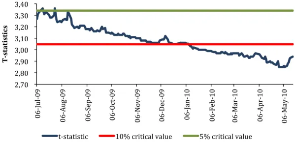
7.2.2 Ending of the Relationship ... 48
7.2.2.1 Results from the Recursive Analysis ... 48
7.2.2.2 Results from the Engle-Granger Test ... 49
7.2.2.3 Robustness Check ... 52
7.2.3 Return of the Relationship ... 52
7.2.3.1 Results from the Recursive Analysis ... 53
7.2.3.2 Results from the Engle-Granger Test ... 54
7.3 Spread Decomposition ... 55
7.3.1 The Landlocked Commodity Spread ... 56
7.3.2 The Transatlantic Commodity Spread ... 56
7.3.3 The Brent Nearby Time Spread ... 56
7.3.4 Factors Behind the Spread ... 56
7.3.5 The West Texas Crude Quality Spread ... 61
7.4 Summing Up: Cointegration and Decomposition ... 62
7.5 Empirical Findings ... 63 7.5.1 Assumptions ... 63 7.5.2 Regression Results ... 66 7.5.3 Analysis ... 68 7.6 Limitations ... 70 7.6.1 Method ... 70 7.6.2 Data ... 71 7.7 Implications ... 73 8. Conclusion ... 75 9. Bibliography ... 77 10. Appendix ... 83
10.1.1 U.S Production and Import ... 83
10.1.3 The Akaike Information Criterion ... 84
10.1.4 Robustness Test ... 84
10.1.4.1 Augmented Dickey-Fuller for Spot Prices ... 84
10.1.4.2 Recursive Analysis for Spot Prices ... 84
10.1.5 Descriptive Statistics of the Spread Decomposition ... 85
10.1.6 The Baltic Dry Index ... 86
10.1.7 Ordinary Least Squares ... 86
10.1.8 Newey-West Standard Errors: ... 88
10.1.9 Testing Coefficients ... 88
10.1.9.1 Testing One Coefficient ... 88
10.1.9.2 Testing Multiple Coefficients ... 89
10.1.10 Open Interest for WTI and Brent ... 90
Figures
FIGURE 1 - SPOT PRICE DEVELOPMENT WTI AND BRENT ... 12
FIGURE 2 – ANNUAL AVERAGE HISTORIC OIL PRICE ... 18
FIGURE 3 - DEMAND SHOCK ... 32
FIGURE 4 - SUPPLY SHOCK ... 33
FIGURE 5 - TWO-REGION MODEL ... 35
FIGURE 6 - SHORT-TERM EQUILIBRIUM ... 37
FIGURE 7 - LONG-TERM EQUILIBRIUM ... 39
FIGURE 8 - RECURSIVE ANALYSIS 2009-2010 ... 49
FIGURE 9 - RECURSIVE ANALYSIS 2013-2014 ... 53
FIGURE 10 - SPREAD DECOMPOSITION 2000-2014 ... 57
FIGURE 11 - SPREAD DECOMPOSITION 2010-2014 ... 58
FIGURE 12 - TOTAL AND WEST TEXAS CRUDE QUALITY SPREAD ... 62
FIGURE 13 – 3:2:1 CRACK SPREADS FOR WTI, BRENT AND LLS ... 74
FIGURE 14 - U.S. PRODUCTION AND IMPORT FROM CANADA ... 83
FIGURE 15 - BRENT SPOT AND OPEC SPARE CAPACITY ... 83
FIGURE 16 - RECURSIVE ANALYSIS FOR SPOT PRICES ... 85
FIGURE 17 - THE BALTIC DRY INDEX ... 86
T
ABLES
TABLE 1 - TYPICAL LIGHT SWEET CRUDE YIELD ... 11
TABLE 2 - API GRAVITY AND SULFUR CONTENT OF WTI AND BRENT ... 12
TABLE 3 - API GRAVITY AND SULFUR CONTENT OF BFOE ... 14
TABLE 4 - API GRAVITY AND SULFUR CONTENT OF LLS AND WTS ... 15
TABLE 5 – SCENARIOS AND ASSUMPTIONS ... 30
TABLE 6 - AUGMENTED DICKEY-FULLER ... 50
TABLE 7 - SECOND STEP ENGLE-GRANGER ... 51
TABLE 8 – AUGMENTED DICKEY-FULLER TEST ... 54
TABLE 9 - SECOND STEP ENGLE-GRANGER ... 55
TABLE 10 - SPREAD CORRELATIONS ... 60
TABLE 11 – AUGMENTED DICKEY-FULLER AND ENGLE-GRANGER RESULTS ... 64
TABLE 12 - REGRESSION RESULTS ... 66
TABLE 13 – T-STATISTICS AND P-VALUES ... 67
TABLE 14 - AUGMENTED DICKEY-FULLER TEST RESULTS ... 84
TABLE 15 - DESCRIPTIVE STATISTICS 2000-2010 ... 85
TABLE 16 - DESCRIPTIVE STATISTICS 2010-2014 ... 85
TABLE 17 - DESCRIPTIVE STATISTICS 2014 ... 86
1.
Introduction
West Texas Intermediate (WTI) has been trading at an unusual discount relative to Brent since 2010. Historically, the two have moved in unison, with WTI trading at a premium to Brent due to its slightly higher quality. Now, however, the two crudes have set on different paths, with WTI experiencing a fall in prices without a corresponding fall in the price of Brent. That two international benchmarks have decoupled from their long-term price relationship could have widespread implications for the oil industry.
We wish to examine the price divergence between WTI and Brent. First we will try to establish when the price relationship between the two ended. If a break is found, we will examine whether it was only a temporary occurrence and if WTI and Brent have formed a new relationship. To further study the unusual price movements, we break down the spread between WTI and Brent into supply and demand components, and build an empirical model to quantify what factors have affected the spread.
The North American benchmark WTI is of great importance in today’s oil pricing system. The crude underlies sweet crude contracts traded at the New York Mercantile Index, and is one of the most significant commodity contracts on the market. Its European counterpart Brent is financially traded on the Intercontinental Exchange in London, and accounts for over two thirds of the world’s total trade in physical oil (Intercontinental Exchange, 2013). As a consequence, Brent is widely referred to as the leading global crude benchmark.
The WTI and Brent benchmarks are integral parts of the crude oil pricing system, comprising the price foundation for nearly all other crudes. The similar qualities between the crudes are key to the benchmarking system, with their price differences being fairly constant. Historically this is said to be true, with WTI being priced $1-4 per barrel above Brent due to its slight quality premium (Carollo, 2011). Bassam Fattouh (2009) contributes the constant price differential between the crudes to the oil market being one great pool. An implication of his theory is that crudes of similar quality will move closely together, as supply and demand shocks that affect one crude should be transferred to others.
The almost constant price differential between WTI and Brent was for a long time a stated fact. However, since 2010 the price differential, or spread, has diverged from its historic trend and Brent is currently traded at a premium to its North American counterpart. The spread reached its peak in August 2011, when Brent traded at a $26 premium to WTI. According to Fattouh’s (2009) research, the prices of the two should behave similarly, with the price fluctuations of one affecting the other. This, however, has not been the case.
Although there is abundance of research, both on the price movements of crude oil and the divergence of the WTI-Brent spread, less research has been conducted towards pinpointing the end of the relationship and examining whether the crudes have formed a new relationship. With the help of econometrical techniques we wish to examine the price relationship between WTI and Brent, as well as quantifying certain effects behind the divergence.
We start by presenting our hypotheses in section 2. A presentation of the properties of crude oil, the modern history of the oil market and a description of the crude oil market is outlined in section 3. We review literature relevant to our thesis in section 4, before presenting specific events that affect crude oil prices in section 5. To easier comprehend crude oil price fluctuations we present a theoretical analysis on crude oil price movements in section 6. Our empirical analysis is presented in section 7 and is divided into sections for our sample data, cointegration analysis, spread decomposition and empirical findings. We discuss limitations and implications of our research in the same section, before presenting our final conclusions in section 8.
2.
Hypotheses
In this section we present and explain our hypotheses. They all originate from the unusual behavior in the spread between WTI and Brent and literature pertaining to the subject.
2.1.1
Hypothesis 1: The Long-Term Relationship
Our first hypothesis is based on the fact that WTI has traded at a discount to Brent since 2010. Historically, WTI and Brent moved in tandem with a spread of $1-4 per barrel in favor of WTI (Carollo, 2011). The reversal in the price relationship could imply that the widely acknowledged long-run relationship between the crudes has ended.
Hypothesis 1a: The long-term relationship between WTI and Brent ended in early 2010.
Between 2010 and 2014 Brent traded at an unusual premium to WTI, but has recently moved towards the once familiar price differential. This may have established a new relationship between the crudes, where WTI is traded at a small discount to Brent.
Hypothesis 1b: A new relationship between WTI and Brent was established at the beginning of 2014.
We also want to determine what caused the unusual behavior in the spread. Crude oil has a physical dimension that anchors its price to fundamentals in the oil market. The unusual price difference between WTI and Brent is therefore likely to be caused by changes in these fundamentals.
2.1.2
Hypothesis 2: The Structural Changes in North America
There are indications that fundamentals in the North American market have caused the price divergence between WTI and Brent. Increasing crude oil production, leading to a greater inflow of crude oil to Cushing, caused storage facilities to reach maximum capacity in 2010. A lack of pipeline infrastructure constrained transportation of the excess crude to coastal refineries, with the combined factors leading to a decrease in the price of WTI.
Hypothesis 2: Increasing crude oil production in North America, as well as insufficient pipeline infrastructure out of Cushing, caused the unusual behavior in the WTI-Brent spread.
In addition to having a physical dimension, crude oil is traded as a financial instrument. Some of these instruments can impact crude oil prices, causing shifts beyond their underlying fundamental value.
2.1.3
Hypothesis 3: The Financial Market Activity
The futures contracts for WTI and Brent are the most traded commodity contracts in the world. In 2011 a relative weight change in favor of Brent in the world’s largest commodity indices allocated large money flows in the financial market from WTI into Brent futures. The relative weight change increased the open interest, an indicator for activity and liquidity in the financial market, for Brent relative to WTI. However, these changes may already be accounted for by market participants and embedded in the prices, and so will not have an effect on the spread.
Hypothesis 3: The open interest for WTI and Brent futures did not have a significant impact on the price divergence between WTI and Brent.
We will test our hypotheses in several sections. In section 7.2 we test the relationship between WTI and Brent with an Engle-Granger two-step test for cointegration. We decompose the spread into time and commodity spreads to understand the underlying shifts in section 7.3. Finally, we present an empirical model to quantify the underlying shifts in section 7.5.
3.
Theory
In this section we present theory concerning the crude oil market and the formation of crude oil prices. Without an understanding of the fundamentals in the crude oil market, it will be difficult to comprehend the implications of our empirical findings.
3.1
What is Crude Oil
1Crude oil is a heterogeneous commodity and its appearance varies, from an almost brown sludge to a light colorless liquid. Fossil fuels, such as crude oil, are non-renewable energy sources, implying that the resource does not renew itself at a sufficient rate for sustainable economic extraction in meaningful human time frames. In its most simple form crude oil consists of molecules and hydrocarbon chains of varying length.
The number of hydrocarbons, in addition to the heat at which the hydrocarbons form, determines the density and classification of the crude oil. The American Petroleum Institute (API) classifies crude oil as either light, medium or heavy in density. The API gravity index is a measure of how heavy or light the crude oil is compared to water. The less dense the crude oil, the higher the API gravity, hence high gravity crudes are known as light crudes while low gravity crudes are referred to as heavy crudes.
Light crudes usually have an API gravity between 35 and 40 degrees. Due to fewer long-chain molecules and lower wax content, it has lower viscosity and is therefore easier to both extract and transport. This leads to lower operating costs for both producers and refiners, which in turn has historically led to higher demand.
Heavy crudes, on the other hand, usually have an API gravity between 16 and 20 degrees. What identifies heavier crudes is higher viscosity and that they contain high concentrations of sulfur and metals. These properties make them difficult to extract and transport through pipeline, making refining more costly.
1 This section is based on Deutsche Bank’s report “Oil & Gas for Beginners” (2013).
2 The assessment of the Brent benchmark is based on the article ”An Anatomy of the Crude Oil Pricing System” written by Bassam Fattouh for the Oxford Instititute for Energy Studies (2011).
In addition to hydrocarbons, all crudes contain sulfur, released on combustion as sulfur dioxide. The sulfur needs to be removed from the oil before refining, leading to higher demand for crude oils with low percentage of sulfur. Crudes containing lower percentage of sulfur are known as sweet, whereas those with high percentage are known as sour. Crude oil is classified as sweet if it contains less than 0.5% sulfur. Light sweet crude oil contains a disproportionate amount of high-quality distillate products and is therefore the most sought after crude.
If the total sulfide level in the crude is over 1% it is defined as sour and contains impurities such as hydrogen and carbon dioxide. Since these impurities must be removed before the crude can be utilized, the cost of refining increases. Due to these increased costs, sour oils are in lower demand and sold with a discount compared to high quality crudes.
Crude oil itself cannot be utilized; it has to be refined into usable products. Refining produces a wide variety of products, from heating oil to petroleum gas. The range of products from a barrel of crude oil is dependent on the quality of the crude. For WTI and Brent a typical yield, the proportion of refined products in one barrel of crude, is shown in table 1.
Table 1 - Typical Light Sweet Crude Yield (Deutsche Bank, 2013)
Not all outputs have the same market value. Some outputs, such as diesel, sell at a premium to heavier fuels. In addition, the heavier outputs tend to be more easily substitutable with other energy alternatives, capping their price movements even at higher crude oil prices.
Product Light Sweet Crude Yield
Petroleum Gas 3 %
Naptha 6 %
Gasoline 21 %
Kerosene 6 %
Gasoil/Diesel (Middle distillates) 36 %
Fuel Oil 19 %
3.1.1
Properties of WTI and Brent
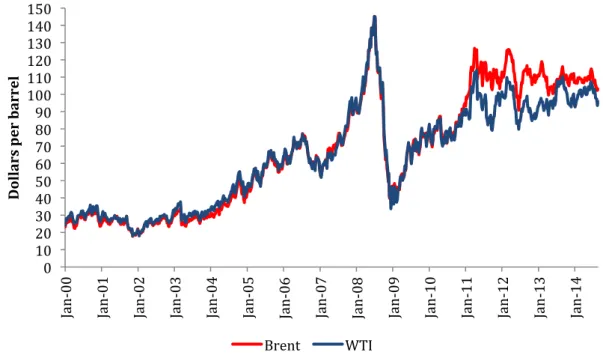
A variety of crude oils are produced around the world with their market value defined by quality characteristics. WTI and Brent are today the key international benchmarks for crude oil, with their prices used as a barometer for a majority of the industry. Their similarities can be seen in the spot price development between 2000 and 2014, where the two move in tandem until 2010. Their price development is depicted in figure 1.
Figure 1 - Spot Price Development WTI and Brent (Bloomberg L.P., 2014e)
To further illustrate, the specific quality characteristics of the WTI and Brent are outlined in table 2. WTI is of a slightly higher quality than Brent as its sulfur content is lower. All else equal, the lower sulfur content implies that WTI should be sold at a slight premium relative to Brent.
Table 2 - API Gravity and Sulfur Content of WTI and Brent (U.S. EIA, 2012b)
0 10 20 30 40 50 60 70 80 90 100 110 120 130 140 150 Ja n-‐0 0 Ja n-‐0 1 Ja n-‐0 2 Ja n-‐0 3 Ja n-‐0 4 Ja n-‐0 5 Ja n-‐0 6 Ja n-‐0 7 Ja n-‐0 8 Ja n-‐0 9 Ja n-‐1 0 Ja n-‐1 1 Ja n-‐1 2 Ja n-‐1 3 Ja n-‐1 4 D ol la rs p er b ar re l Brent WTI
Crude Oil API Gravity Sulfur Content
WTI 39.6° 0.24%
3.1.1.1
The Brent Benchmark
2The crudes comprising the Brent benchmark is extracted from the North Sea and acts as a representative for a wide variety of crudes. Brent as a benchmark has evolved from one single crude representing the whole North Sea, to a mix of several crudes. Brent was the first crude to act as a representative for the North Sea, and is a mixture of oil produced from several fields delivering to the terminal at Sullom Voe in the Shetland Islands, United Kingdom. As production started to decline in the 1980s, Brent was comingled with Ninian to stop opportunities of manipulation and distortion. The new benchmark was named Brent Blend.
Brent Blend was used as a benchmark until 2002, when production hit an all-time low. In order to counter this, the Brent Blend was broadened to include Forties and Oseberg. The new benchmark was known as Brent-Forties-Oseberg (BFO). With the inclusion of these two crudes it resulted in a distribution over a wider range of companies, reducing the dominance of oil producing companies and decreasing opportunities to distort the benchmark.
In 2007, Ekofisk was included in the benchmark, leading to the creation of the benchmark that is in use today, Brent-Forties-Oseberg-Ekofisk (BFOE). The inclusion of Ekofisk increased the physical base of the benchmark, and is the status quo of today.
The inclusion of the different crude oils with diverse quality aspects has had implications on the pricing of the benchmark. Any of the four crudes can be delivered against a BFOE contract, and thus sellers wish to deliver the cheapest grade of crude. In the BFOE blend, Forties has the lowest quality with regard to API and sulfur content and thus sets the price and quality grade of the benchmark.
2 The assessment of the Brent benchmark is based on the article ”An Anatomy of the Crude Oil Pricing System” written by Bassam Fattouh for the Oxford Instititute for Energy Studies (2011).
Table 3 - API Gravity and Sulfur Content of BFOE (U.S. EIA, 2012b)
There are several aspects that favor the choice of Brent as a benchmark. Brent is seaborne and can be transported to refineries in Europe and other parts of the world when arbitrage opportunities deem transportation profitable, making it easily marketable. The geographic location makes it an ideal benchmark as the North Sea is close to refineries both in Europe and the United States (U.S.). With four different crudes constituting the benchmark, the large production volume makes it difficult to manipulate.
However, it is not just the volume of production that makes it an ideal benchmark. An important aspect is that the United Kingdom’s government acts as an overseer for Brent, providing a transparent legal and regulatory body. In addition, due to its inclusion of several crudes, no producer has monopoly on the blend, which is one of the most important aspects of a benchmark (Horsnell & Mabro, 1993).
The Brent benchmark sets the price for most of the global crude market, which underlines its importance. Around 70% of the world’s crude is priced relative to the Brent benchmark (RBN Energy, 2013).
3.1.1.2
The WTI Benchmark
3WTI has its origin in the crude oil fields of Texas, Oklahoma, Kansas and New Mexico. The crude oil is landlocked, as opposed to the seaborne Brent, and is thus subject to domestic infrastructure problems. Deliveries of the crude are made to Cushing, Oklahoma, which is strategically placed to serve the refineries along the Gulf of Mexico.
3 The assessment of the WTI benchmark is based on the article “An Anatomy of the Crude Oil Pricing System” written by Bassam Fattouh for the Oxford Institute for Energy Studies (2011).
Crude Oil API Gravity Sulfur Content
Brent Blend 38.3° 0.37%
Forties Blend 40.3° 0.56% Oseberg Blend 37.8° 0.27% Ekofisk Blend 37.5° 0.23%
The U.S. market consists of several crudes besides WTI. One of these crudes is the Light Louisiana Sweet (LLS), which has become a local benchmark for sweet crude along the Gulf Coast. LLS is seaborne and can easily be transported to meet world demand or stockpiled cheaply on floating storage facilities, making it less exposed to the domestic problems WTI might experience. LLS is of similar quality to WTI and Brent. Another crude oil of significance in the U.S. is the West Texas Sour (WTS), a lower quality crude being stored at Cushing, OK. Both crudes’ qualitiy aspects are depicted in table 4.
Table 4 - API Gravity and Sulfur Content of LLS and WTS (U.S. EIA, 2012b)
Despite there being a wide variety of crudes, WTI has become the main benchmark for pricing crude in the U.S. This is because WTI underlies the Light Sweet Crude Oil futures contract, one of the largest and most actively traded commodity futures contract. In addition, WTI is traded in smaller volumes than other crudes, making it easier for investors to find the necessary credit and storage facilities to participate in its trading. Furthermore, its liquidity is high, solidifying it as an apt benchmark for the U.S. crude market (CME Group, 2010).
Unlike Brent, WTI has seen a surge in production, especially from unconventional oil from Canada and the U.S. A surge in crude oil prices over a prolonged period spurred innovations that lead to these resources becoming economically viable. Unconventional oil represented a major shift in supply side conditions, with North American crude production accounting for 14% of global crude production in 2012 (Erbach, 2014).
Canada has large deposits of oil sand, representing the largest undeveloped, oil resource globally. These reserves contain heavy, thick deposits of bitumen-coated sand, which require significant amounts of energy, making its extraction capital intensive.
Crude Oil API Gravity Sulfur Content
LLS 35.6° 0.37%
The unconventional oil deposits in the U.S. are mainly tight oil from the Bakken field in North Dakota and the Eagle Ford Plays in Texas. Tight oil is a subset of tight hydrocarbons with the key, differentiating factor being that its reservoir rock, shale, is also the source rock for the oil.
3.2
Modern History of the Oil Market
4The current oil pricing system has emerged in response to changing power balances, shifts in political and economic structures, as well as fundamental changes to supply and demand. It has gone from a monopolistic pricing system to the market based system we know today.
Until late 1950s the oil price was controlled by multinational companies, known as the Seven Sisters5, who accounted for 85% of the oil production outside Canada, the U.S., the USSR and China. These multinationals had interests in both up- and downstream production, owning the whole value chain from exploration to refining. Governments received royalties and taxes, but did not participate in pricing the oil. Until the 1970s the pricing system, known as the posted price, was built on these royalties. The period was characterized by a market with few participants and imperfect competition, where multinational companies set prices to minimize their tax liabilities around the world.
In 1960 the Organization of the Petroleum Exporting Countries (OPEC) was formed by Iran, Iraq, Kuwait, Saudi Arabia and Venezuela to coordinate tax and royalty policies, obtain resources from private companies, as well as preventing declining revenues for its members. Even though large multinational companies still dominated the market in the 1960s, smaller independent companies were entering the market. This was due to the fact that countries, like Venezuela and Libya, granted concessions to smaller participants as they saw an opportunity to gain higher government tax and royalties.
4 This section is sourced from “An Anatomy of the Crude Oil Pricing System” written for the Oxford Institute for Energy Studies by Bassam Fattouh (2011).
5 Anglo-Persian Oil Company (now BP), Gulf Oil, Standard Oil of California (SoCal), Texaco (now Chevron), Royal Dutch Shell, Standard Oil of New Jersey (now Esso) and Standard Oil Company of New York (Now ExxonMobil).
In the period between 1965 and 1973 the global demand for oil increased rapidly. As a response, OPEC increased production to meet the surging demand. In 1973, in response to having gained a significant share of the world crude market, power shifted in favor of OPEC as they for the first time sat a posted price.
During the 1970s the concept of marker price was introduced, a predecessor to what is now known as crude benchmarking. This further shifted the power of oil pricing from the multinational companies to OPEC. Arabian Light from Saudi Arabia was chosen as the first marker crude and prices were set relative to this.
The Iranian crisis in 1979 led to an abrupt disruption in the supply of crude oil. This forced multinational companies to buy crude in the open market to meet their refineries’ demand. As a consequence, a new spot market emerged with higher transparency, making it easier for non-OPEC countries and private companies to establish themselves in the oil market.
In the early 1980s, OPEC increased its production in response to higher crude oil prices. However, the worldwide recession in the mid 1980s caused a decline in the demand for oil. This represented a major challenge to OPEC’s marker pricing system, ultimately leading to its demise.
Another factor leading to the demise of OPEC’s marker pricing system was that more oil reached international markets as non-OPEC members made new discoveries and increased production. As non-OPEC members priced their oil to market conditions, they were able to charge a lower price for their crude compared to OPEC. Suppliers, who had an excess of crude, undercut prices in the spot market, ultimately leading to a decline in the demand for OPEC crude.
As it became clear to OPEC that attempts to defend the marker price would only result in a lower market share, they adopted a new pricing system, the netback pricing system. Other oil exporting countries adopted the system, which provided companies with a guaranteed refinery margin. This led refineries to oversupply the market with refined products, leading to the oil price collapse in 1986.
After the crisis a new market system for pricing crude oil emerged, known as formula pricing. The system is an arrangement where a buyer and seller agree in advance on the price to be paid for a product delivered in the future. This benchmark price is based upon a pre-determined calculation, and is still in use today. OPEC abandoned its netback pricing system and adopted the new market system, and so transferred the pricing power to the market.
In 1988 the new market related pricing system was widely accepted amongst most oil-exporting countries. In the subsequent years the technological revolution made electronic 24-hour trading possible from anywhere in the world. The revolution enabled the development of a complex pricing system of interlinked oil markets, consisting of spot, physical forwards, futures and other derivatives in the paper market.
With the exception of the time period around the Iranian crisis in 1979, crudes prices normally fluctuated around $20 to $30 per barrel. However, since 1998, crude prices have soared to a record high of $145 in July 2008, before falling during the financial crisis. At the time of writing, WTI and Brent is traded at around $70 dollar per barrel. The annual average of the historic oil price is depicted in figure 2.
Figure 2 – Annual Average Historic Oil Price (Inflation Data, 2014)
0 10 20 30 40 50 60 70 80 90 100 110 120 1946 1948 1950 1952 1954 1956 1958 1960 1962 1964 1966 1968 1970 1972 1974 1976 1978 1980 1982 1984 1986 1988 1990 1992 1994 1996 1998 2000 2002 2004 2006 2008 2010 2012 D ol la rs p er b ar re l
3.3
World Oil Markets Today
The global oil market is the largest energy market, measured in both value and volume. In 2011 crude oil served around 33% of the global energy needs (Deutsche Bank, 2013).
The New York Mercantile Index (NYMEX) and the Intercontinental Exchange (ICE) are the main international exchanges for the trading of crude oil. The exchanges allow for trade in both the spot market for immediate delivery and the forward and futures market for deliveries at a predetermined date. This provides market participants with hedging, speculation and price discovery opportunities.
Due to the large number of crudes around the world, benchmarks are widely used to set prices, both for physical delivery and in the financial market. The two most important are, as previously mentioned WTI and Brent. All other crudes, with some exceptions, are traded at a discount or premium to these benchmarks, depending on their quality aspects, as explained in section 3.1.
3.3.1
Futures Market
Futures trading, as we know it today, evolved when farmers and merchants committed to future exchanges of grain for cash in the 19th century. A century later, in 1983, NYMEX introduced trading in crude oil futures with delivery of light sweet crude oil at Cushing, Oklahoma. A few years later the International Petroleum Exchange, now ICE, introduced futures trading in Brent derivatives (Gülen, 1998). Since the introduction of formula pricing in 1988, and the technological development of trading, futures have played an increasing part in pricing crude oil deliveries, and has evolved into a foundation for determining spot prices for North American crude (Deutsche Bank, 2013).
The largest exchange-traded commodity in the world was for a long time WTI, trading at a volume nearly four times that of Brent (Clayton, 2013). The futures contract is often bought by refineries located on the Gulf Coast and in the mid-continent of the U.S., and is thus highly sensitive to regional supply and demand factors.
Due to the liquidity of the WTI futures contracts and the fact that the U.S. is the largest oil consumer globally, WTI is of great importance and a point of reference for the domestic market (U.S. EIA, 2014b). In addition, futures contracts for WTI are the best visible real-time reference price for the market. Negotiations in the spot market will therefore use the futures price as a reference point (Platts, 2010).
The Brent futures contract traded on ICE surpassed the WTI contract in 2013, and is today the largest traded crude oil future in the world (Clayton, 2013). Brent futures are, unlike WTI, settled financially. The settlement is a weighted average of all trades in the physical market for the month in question for each underlying component of the Brent benchmark. The financial instrument is far more complex than WTI, due to the inclusion of four crudes, Brent-Forties-Oseberg-Ekofisk, in one instrument (Fattouh, 2011).
Crude oil has, unlike pure financial assets, a physical dimension that anchors expectations to fundamentals of the oil market. Every day millions of barrels are bought and sold at prices determined in the market. By the law of one price a good must sell for the same price in all locations, and thus the futures market should eventually converge with the spot market to remove the possibility of arbitrage. However, if perceptions of future market fundamentals are uncertain, exaggerated or both, the futures market can diverge away from the underlying fundamental value and create a bubble (Deutsche Bank, 2013).
Market participants use the futures market in different ways to make a profit or hedge against loss. Commercial traders, producers and consumers of crude and refined products, optimize their portfolio by hedging exposure. Mainstream institutional and retail investorstrade in the market to profit from movements in the price, often known to be hedge funds or pension funds. Traders and commodity trading advisor’sattempt to profit from price deviations between regions and commodities or to anticipate the future price of crude oil (Deutsche Bank, 2013).
3.3.2
Forward Curve
The forward curve is the series of sequential prices for future delivery of crude oil or expected future settlements of an index. It has increased in importance along with the
growing financial market, with expectations of supply and demand being reflected in the curve. An upward sloping forward curve indicates higher prices in the future. This again indicates that one expects demand to increase more relative to supply, that supply is going to tighten, or that spare capacity of crude oil is more limited in the future.
An upward sloping forward curve, referred to as contango, where the futures price of a commodity increase with time, is considered normal, stripped from all expectations of future demand and supply. This is due to the fact that cost of carry, i.e., the cost of storing the crude, is included in the curve and thus the price will be higher for future delivery. If the curve slopes downwards, referred to as backwardation, it implies that the market expects either demand to decrease more relative to supply, a surge in supply or that the spare capacity of crude oil is less limited in the future (Deutsche Bank, 2013).
4.
Literature Review
In this section we present relevant literature for our thesis. We review literature regarding the pricing of non-renewable resources, and more specifically WTI and Brent. Literature pertaining to the crude oil markets and the WTI-Brent spread is also presented. Based on the literature review we give a brief discussion on how we utilize earlier research in our thesis.
The pricing of crude oil has been widely reviewed by several papers (see e.g. Hotelling, 1931; Horsnell & Mabro, 1993; Bacon & Tordo, 2004; Hamilton, 2008; Carollo, 2011; Amadeo, 2014). All reviews are based on the fact that crude oil is a finite resource; meaning that at some point in time oil reserves might be depleted. It was Harold Hotelling who first described the evolution of non-renewable resource pricing. In his article “The Economics of Exhaustible Resources” from 1931, Hotelling states that the price of a finite resource must rise at a rate equal to the discount rate, known as the Hotelling’s rule or scarcity rent. He also showed that in competitive markets, his rule maximizes the value of the resource stock. As a consequence, all else equal, the price of crude oil must rise and continue to rise in the future.
However, Hotelling’s model does not fully reflect reality, as his assumptions are simplifications of the real world. Hotelling assumes perfect competition and that the stock is fully known. Further, he assumes that the resource extracted is used completely with no waste, nothing left for reuse and that there are no externalities or market failures. Lastly, Hotelling assumes that the cost of extraction is constant and that there are no alternatives to the resource.
Hotelling’s model has been extended in various ways in later papers. Krautkraemer (1998) finds that the Hotelling model has not been consistent with empirical studies of non-renewable resource prices, as there has not been a persistent increase in prices over the last 125 years. His review emphasizes that, as non-renewable stocks are not known, technological progress that lowers the cost of extraction and processing, and the discovery of new deposits, has played a greater role than finite availability in pricing renewable resources. His empirical analysis also proves that non-renewable resources often have usable residuals from production, and thus must be calculated in the total price of the non-renewable resource.
In a theoretical analysis in the same research paper, Krautkraemer reviews the effects of backstop technology on the price of non-renewable resources. As a finite resource increases in price, other alternative resources, backstops, will become relatively cheaper and thus preferable for consumers. He also illustrates how heterogeneous quality aspects affect the price of a non-renewable resource. Based on his review, Krautkraemer extends the basic model to account for these factors.
Recently, attention has been focused towards incorporating the issue of climate policy in the Hotelling model. Kolstad and Toman (2001) argue that crude oil prices should reflect climate issues, and modifies the model to take into account how increased greenhouse gas emissions causes reduction in welfare over time.
Hotelling’s model and later research on the subject have provided a deeper understanding of how prices of non-renewable resources are formed. Thus, the intuition behind the model and its extensions is essential when interpreting our empirical analysis based on the price divergence between WTI and Brent.
Hamilton (2008) surveys crude oil prices in the period between 1970 and 2008. He attributes strong growth in demand from emerging economies, coupled with a failure of global production to increase, as reasons behind the exuberant rise in oil prices since 2000. However, his article does not examine specific crude prices, only general crude price movements. A natural extension of Hamilton’s work would be to study specific crudes, such as WTI and Brent, seeing as not all exogenous factors move crude prices with the same strength. Our thesis will build on Hamilton’s research and extend the time period analyzed to capture the shale oil revolution in the U.S., and its impact on crude oil prices.
In an extensive research effort by Kilian (2009; 2014), crude oil prices were retrieved back to 1975 and decomposed to examine whether historical oil price shocks could best be explained by demand or supply conditions. The three-way decomposition consisted of (i) crude oil supply shocks (ii) increased aggregated, global demand for all industrial commodities and (iii) a preventative increase in demand for crude oil. Kilian finds that demand conditions has the largest effect on price fluctuations, both in the short and long-term. His findings broke with earlier supposed truisms, that supply conditions best could explain oil price movements. In our empirical analysis, we use these findings by decomposing the spread to study whether the divergence between WTI and Brent can be explained by supply or demand conditions.
In an empirical study of the global crude market, Nordhaus (2009) concludes that the crude oil market is integrated, where the sum of total demand and supply and inventory levels determine the price. Nordhaus emphasizes the fact that crude oils from different geographic regions are largely interchangeable when of similar quality. They are as such fungible; shipping the same or similar oil from elsewhere can make up for a shortfall in a specific region. However, his findings do not imply that short-term deviations from a more or less constant long-run relationship between crudes signify an ending of a relationship. As Balke and Fomby (1997) observe, due to the existence of adjustment and transaction costs, movements toward the long-run equilibrium do not occur in a linear fashion or instantaneously. In our work we wish to examine if the divergence in the WTI-Brent spread is only a short-term occurrence and whether prices are moving back towards their long-term relationship.
To examine whether there is a long-term relationship between WTI and Brent prices, Reboredo (2011) uses a copula approach. His paper examines the dependence structure between crude oil benchmarks, suggesting that crude prices co-move and are linked with the same intensity during bear and bull markets. These findings support Nordhaus’ (2009) conclusion of the crude oil market being one great pool. However, these articles do not examine the reasons behind the co-movements. As WTI and Brent have diverged from their long-term price relationship, we extend their research and study what affects WTI and Brent prices, and if their relationship has altered. The claim that the crude market is one globalized pool is backed up by arbitrage theory. Several empirical papers (see e.g. Hamilton, 2008; Fattouh, 2011) as well as theoretical papers (see e.g. Schwarz & Szakmary, 1994; Al-Loughani & Moosa, 1995; Bacon & Tordo, 2005) have supported this claim. Their results indicate that the world crude oil market, in the long run, is a large integrated market where prices co-move. These results imply that price differences between crude oils should reflect quality differences and transportation costs in the long run. The recent divergence between WTI and Brent has, at least in the short term, disproved this theory, and we therefore examine the factors behind the divergence.
Theoretical research supporting the case for a globalized crude oil market has been empirically tested. Fattouh (2009) finds, with the help of standard root tests, that crude oil prices cannot deviate without restrictions and are thus linked, confirming the globalization theory. One implication of Fattouh’s research is that crudes of similar quality in different markets should move in unison such that their spread is more or less constant in the long run. He presents a relationship between WTI and Brent built on his assumption of the crude oil market being one globalized pool, formally:
𝑃!",!+𝐶!"+𝐷 =𝑃!"#,! (1)
Here 𝑃!" and 𝑃!"# are the prices for Brent and WTI at time t, 𝐶!" represents the cost of carrying Brent and D is the quality discount. If the WTI-Brent differential is greater than zero it will lead to arbitrage, i.e., U.S. refineries will import Brent, and continue to do so until the price relationship is again attained. Fatthouh’s findings are in
contrast to what has recently occurred in the spread between WTI and Brent, where WTI has been sold at a discount to Brent over a prolonged period of time. This has led us to postulate a new price relationship between the crudes:
𝑃!",!+𝐶!"+𝐷+𝑆=𝑃!"#,! (2) Based on our hypothesis, we have added a term, S, to capture structural changes in North America. In our empirical analysis we will quantify the factors that has affected the spread. If these have a significant affect, it will give validation to our extended model.
In an earlier paper, Fattouh (2007) claims that the long-term price relationship between WTI and Brent started to show signs of weakness already in 2006. He implies that pipeline logistics and the insufficient of infrastructure is a significant factor in what he terms as a breakdown of the WTI price. Fattouh also highlights the fact that Brent is a seaborne crude, as opposed to WTI, and hence does not suffer from the same pipeline bottlenecks. However, these findings are not based on statistical evidence, but rather on descriptive data on the price movements of WTI. An empirical analysis would have strengthened the conclusions of Fattouh. Further, his article was written in 2007, and is thus outdated given recent events. We add to Fattouh’s observations by formally testing his findings by using cointegration analysis to see whether the long-run relationship between WTI and Brent has temporarily ended.
In an analysis of the WTI-Brent spread, Büyükşahin et al. (2012) find that WTI has periodically traded at what they refer to as unheard of discounts to Brent since the fall of 2008. They find structural breaks in the long-term relationship in 2008 and 2010 and provide empirical evidence using an econometric model where financial and macroeconomic variables help predict the observed spread levels. Our thesis builds on these structural breaks in the relationship, but use a cointegration approach to formally examine if WTI and Brent were in a long-term relationship. We wish to empirically test the divergence in the spread by decomposing it into time and commodity spreads. We extend their research by testing an updated data sample and
quantifying what factors caused the recent price divergence between WTI and Brent. In addition we examine whether the two crudes are back in a long-term relationship, an occurrence Büyükşahin et al. did not test for.
In the same research paper, they also examined if financial aspects caused a structural break between WTI and Brent. Two major indices for commodities, the Standard & Poor’s GSCI commodity index and Dow-Jones UBS commodity price index shifted its relative crude oil exposure away from WTI over to Brent. These two indices are the most widely used benchmarks for commodity index funds, and the shift towards Brent caused large money flows from WTI into Brent futures. Büyükşahin et al. finds evidence for a structural break in the WTI-Brent spread in December 2010. This result is a good indicator for a possible ending of the long-term relationship between the two crudes, and their findings lead us to empirically test whether the financial market has had a significant effect on the spread between WTI and Brent.
5.
Events that Affects the Oil Price
As the presented theory and literature has shown, there are several factors that move the price of WTI and Brent, both independently and simultaneously. However, the theory presented in the literature review can only explain oil price movements up to a certain point. We present specific events that affect crude prices. In addition, we also present specific events that affect the prices of WTI and Brent individually, as they are produced in separate parts of the world, and will thus be influenced by local occurrences. These events will be implemented in our empirical research.
5.1.1
Events that Affect Prices Simultaneously
Economic growth has a positive effect on all crude prices. In the build-up to the financial crisis in 2008, low interest rate policies led to excess liquidity and economic growth that put upward pressure on crude prices. With the collapse of Lehman Brothers and the following financial crisis, the sudden evaporation of economic growth was followed by a reduction in the price of crude. In our empirical model we account for both the U.S. and world economy to control for shifts in economic growth.
The commodity market is highly linked to stress stemming from global financial markets. In times of high levels of financial stress, demand declines leading to decreased commodity prices. We control for this in our empirical model by isolating fluctuations in demand stemming from financial stress.
Lighter crudes, like WTI and Brent, are usually sold at a premium relative to the heavier crudes. This light-heavy spread reflects the yield produced from distillation. The fact that lighter products are in higher demand, forces an upward shift in the price of lighter crudes in times of tightness in the crude oil markets. This is augmented by the fact that spare capacity in the market is mainly from producers of heavy crude. They can alleviate the tightness in the market, but not satisfy the demand for lighter products. This in sum has the implication of increasing the light-heavy spread in tight markets. When decomposing the spread into different components, we examine the light-heavy spread between WTI and WTS to study if there are spillover effects from the unusual behavior in the WTI-Brent spread.
Certain economies with excess supply of crude keep oil in reserve or adjust production for political or economic reasons. OPEC and the U.S. hold reserves to be able to have spare capacity on hand for market management. Both reserves are readily available and can change supply in the market, altering the price of crudes and distillate products in a way the countries see fit. In addition, Saudi Arabia, the largest producer in OPEC, adjusts production for political or economic reasons. The U.S. and Saudi Arabian crude production, and OPEC spare capacity, is controlled for in our empirical model, as they affect prices of both Brent and WTI.
5.1.2
Events that Influence the Price of WTI
The growing inflow of crude oil to Cushing, as a response to increased production in North America, explained in section 3.1.2, led storage facilities to almost reach peak capacity. This has induced the expansion of storage capacity, doubling Cushing’s storage to meet the increased production (CME Group, 2010). Additional capacity prompted the increased trading of WTI, solidifying Cushing as a trading hub of great importance. In addition to the increased capacity, pipelines were built to increase the influx of crude. In total, this has managed to alleviate pressure on pipeline infrastructure into Cushing and its surrounding storage facilities.
However, the production of pipelines to shift crude out of Cushing has not kept the same pace. Between 2010 and 2013 capacity for delivering crude to Cushing increased significantly due to the construction of pipelines, such as the TransCanada Keystone pipeline that originates in Alberta, Canada. The growing supply of crude oil to Cushing far surpassed the surrounding refinery and pipeline take-away capacity. This has resulted in a bottleneck in Cushing, causing a large build-up of crude and depressing the WTI price (Genscape, 2014). We empirically test whether these pipeline and capacity issues have had a significant impact on the spread and its unusual behavior.
Local weather conditions can also have an effect on the WTI price. The Gulf of Mexico and the Southern U.S. has witnessed extreme weather such as hurricanes. In 2005 hurricanes forced refineries and production sites along the Gulf Coast to shut down, which immediately increased the price of WTI as supply dropped (U.S. EIA, 2014d). As we wish to test for certain supply conditions in North America, we need to isolate drops in supply stemming from these weather conditions. We therefore control for hurricanes in our empirical model.
5.1.3
Events that Influence the Price of Brent
Brent, as opposed to WTI, is a seaborne crude, making it more sensitive to demand from global and emerging markets. After Japan shut down its nuclear facilities after the Fukushima incident in 2011, their demand for fossil fuel greatly increased. These factors put upward pressure on the Brent crude price (The Economist, 2011). In our empirical model we account for factors that affect the demand for seaborne crudes, by both including the immediate demand for Brent and world economic activity.
The demand for Brent has also been affected by geopolitical situations. With the Tunisian revolution and the subsequent political turmoil during the Arab Spring, crude oil supplies from these areas have been under risk. The Libyan crisis removed a large supply of sweet crude, and the continuing turmoil in other parts of the Middle East have put production facilities under duress. As Brent is a close substitute to these crudes, this has put upward pressure on the price. In our empirical model, we account for political unrest to isolate the fluctuations caused by supply disruptions and the risk premium added by investors.
6.
Stylized Theoretical
Analysis
In the following section we use the theory presented so far and apply it in a theoretical framework to easier comprehend why crude prices fluctuate. The focus of our stylized theoretical analysis will be on the North American market, as we hypothesized that the problems in Cushing have been the main driver behind the divergence between WTI and Brent. In the presentation of each scenario, we apply the theoretical framework to real life occurrences, which will be a useful backdrop when interpreting our empirical analysis in section 7. Before we present our theoretical analysis, we address certain assumptions that are inherent throughout all scenarios.
6.1.1
Assumptions
The depiction of the crude oil market is static and focuses only on short-term effects. In the long run, quality differences and transportation costs determine the price. The market for crude is global, with no regional differences. These assumptions are supported by previous research, as discussed in the literature review. We further assume that the market is perfectly competitive, with no supplier or consumer having any form of market power.
Two types of crude oil supply the market. Seaborne crude from the North Sea referred to as Brent and landlocked crude sourced in Cushing, referred to as WTI. The price of Brent is a proxy for world price in our scenarios. The crudes are assumed to be aggregated and thus depict the market as a whole. Due to the small quality differences between WTI and Brent, we assume them to be identical products with no switching cost for the buyers.
We depict two markets in our theoretical analysis. The first is the inland North American market, denoted Landlocked, representing the crude oil market north of Cushing. The second market is the market south of Cushing, denoted Seaborne, able to utilize WTI, Brent or a combination.
The landlocked crude, WTI, faces capacity constraints from its selling point Cushing to the Seaborne market. Pipelines that supply Cushing with oil have enough capacity to handle increased supply, whereas the pipelines that transport oil out of Cushing to
the Seaborne market does not have the ability to handle increased production. This implies that demand for crude in the Seaborne market can only be supplied by WTI up until the point of maximum pipeline capacity. The vertical line denoted capacity constraint illustrates this.
We illustrate several scenarios to depict how crude oil prices are affected by exogenous changes in supply and demand. First we present two scenarios that illustrate how supply and demand shocks affect the price of WTI in the Seaborne market without the possibility of importing Brent. We subsequently expand both scenarios to account for capacity constraints at Cushing. The next scenario depicts the Landlocked market’s ability to shift WTI to the Seaborne market, with and without capacity constraints. In this scenario we allow for the import of Brent. Finally, we present a cost-differential model, where the short-term assumption is eased to examine how different modes of transportation to the Seaborne market can affect the price and quantity supplied of each crude.
All scenarios are based on the assumption that the market is in equilibrium prior to any exogenous change. Furthermore, we assume downward sloping demand functions, illustrating the fact that demand falls with rising crude oil prices. The supply curve is upward sloping, reflecting increasing costs as output increases.
Table 5 gives an overview of the different scenarios. Table 5 – Scenarios and Assumptions
Assumption
Capacity Constraint Without With Without With Without With With
Landlocked Perspective x x x
Seaborne Perspective x x x x x
Isolated Market x x x x
Brent Price Given x x
Demand Shock Supply Shock Two-Region Model
Long-Term Equilibrium
6.1.2
Demand Shock
The first scenario illustrates the effect of a positive demand shock to the Seaborne market. We assume the market is isolated in that only WTI can be supplied and discuss the scenario with and without capacity constraints. The effects are illustrated in figure 3.
Without constraints, a positive shock will increase demand for crude oil in the Seaborne market, increasing quantity, regardless of price. This relates to a positive shift in the demand curve, increasing both the price and quantity demanded of WTI, from [Po, Q0] to a new equilibrium [P1, Q1].
However, with a constraint, the inability to increase supply out of Cushing to the Seaborne market will have a feedback-effect on the price. Consumers will outbid each other to gain access to the limited supply of WTI crude, increasing its price above what would have been the market price without capacity constraints. The price increase will continue until the market is again at equilibrium, with higher prices and no change in quantity [P2, Q0]. The feedback effect arises because at the quantity supplied, marginal willingness to pay is higher than marginal cost. Hence, consumers outbid each other until equilibrium is established where marginal cost equals willingness to pay.
Figure 3 - Demand Shock
The market for WTI has over the last decade experienced increased demand without being able to supply the market south of Cushing with crude. The U.S. demand for oil has grown almost every year, increasing pressure on Cushing to pump oil to the market. Without pipeline expansion from Cushing to refineries on the coast, the bottleneck will have the effect of increasing prices for WTI, all else equal.
6.1.3
Supply Shock
This scenario depicts the effects of a positive supply shock to the Seaborne market. As in the first scenario, we assume that the Seaborne market is isolated and we discuss the scenario with and without constraints. The effects of a supply shock are illustrated in figure 4.
A positive shock to supply without capacity constraints increases the supply of oil to the Seaborne market. The supply curve experiences a positive shift, decreasing prices
but increasing the quantity supplied. The market is now in a new equilibrium, moving from [P0, Q0] to [P1, Q1].
With capacity constraint, a supply shock will decrease WTI prices further. Again we assume that the market is in equilibrium at [P0, Q0] prior to the supply shock. With increased supply of WTI, no increase in demand and a capacity constraint, competition between producers will cause a decrease in price. As the increased supply into Cushing cannot be supplied to the Seaborne market, competition increases further as oil producers with low marginal cost cut prices to keep market shares. This feedback effect gives rise to a new equilibrium at [P2, Q0] with the same quantity consumed, but at a lower price.
Figure 4 - Supply Shock
WTI has been subject to increased production volumes due to the unconventional oil revolution in North America. As a consequence, producers were eager to expand pipeline capacity into Cushing, leading to a rush in pipeline construction. Amongst
the projects was the Keystone XL pipeline in 2011 (Reuters, 2013). Though pipelines leading into Cushing increased, pipeline projects sending oil out were insufficient in handling the increased crude volumes. This led to large accumulations of oil at Cushing, leading to a depression of the WTI price.
6.1.4
Capacity Constraints in a Two-Region Model
In this scenario we depict the Landlocked market’s ability to shift WTI to the Seaborne market. The Seaborne market has the possibility of consuming WTI, Brent or a combination of the two. We assume that the price of Brent is given, as the quantity shifted from the Landlocked to the Seaborne market has little or no impact on the world price. It is assumed that the price of Brent is higher than WTI as the glut of oil in the Landlocked market has depreciated prices relative to Brent. We will discuss the scenario with and without capacity constraints to illustrate the effects of a pipeline bottleneck on the WTI price. The initial equilibrium in the Landlocked market is [P0, Q0], before we open for the possibility of shifting oil to the Seaborne market. All effects are illustrated in figure 5.
Without a constraint on the possibility of shifting oil to the Seaborne market, producers of WTI will increase their production until the cost of the marginal producer equals the price of Brent. This will lead to an increased production of WTI equal to [Q2], with producers being able to charge the world price, [PBrent]. The new
equilibrium in the Landlocked market is [PBrent, Q1], with producers of WTI supplying [Q2-Q1] to the Seaborne market.
If the same scenario is depicted with capacity constraints, the Landlocked market can only shift oil to the Seaborne market until maximum capacity. This will constrict the supply of WTI to the Seaborne market, having the effect of decoupling WTI and world prices. The effect of the constraint is that producers with lower marginal costs will decrease prices to stay competitive. With the constraint producers can only increase production to [Q4], obtaining price [P1]. This leads to a new equilibrium in the Landlocked market [Q3, P1], with the Seaborne market being supplied with [Q4-Q3] from producers of WTI.
Figure 5 - Two-Region Model
This scenario illustrates the price divergence that has occurred in recent years between WTI and Brent. With increasing volumes of unconventional oil flowing into Cushing, without the same possibility of shifting it to consumers south of Cushing, prices diverged. This resulted in an increased inflow of other crudes to the Seaborne market to saturate demand.
6.1.5
Long-Term Equilibrium
We are also interested in examining the effects of a capacity constraint when the short-term assumption is eased and increase the number of transportation alternatives. We will look at both the marginal costs of transporting WTI from the Landlocked to the Seaborne market and the marginal cost of transporting Brent. The model depicts the different marginal cost per barrel to illustrate the price spread. The model itself does not predict a price spread between the crudes, but is implied in the transaction. We will first depict the short-term market where only pipelines are able to transport
WTI, before we ease the short-term assumption and include other means of transportation.
The marginal cost of shifting oil through pipelines from the Landlocked to the Seaborne market is initially lower than the marginal cost of Brent, reflecting the fact that pumping oil through existing pipelines is almost perfectly elastic. However, when maximum capacity is reached, the marginal cost curve is kinked 90 degrees, implying that supply is perfectly inelastic. As a consequence, producers of WTI can only supply [QPipeline] to the Seaborne market in the very short run.
The seaborne Brent has a higher marginal cost than WTI, as new tankers are required to transport additional crude. We assume no shortage of oil tankers, as Brent is not affected by the same capacity constraints as WTI. For each additional tanker hired, the price of carry by sea will rise, increasing marginal costs.
Given these assumptions, producers of WTI can only supply the market with [QPipeline], while the producers of Brent supply the remaining demand [QBrent-QPipeline] in the very short run. Even if the marginal cost of production for WTI is lower than Brent, it is unable to be transported to the coastal market where it can be sold at world prices. This is illustrated in figure 6.