Asymmetric Multivariate Stochastic Volatility
∗Manabu Asai
Faculty of Economics Soka University
Michael McAleer
School of Economics and Commerce University of Western Australia
Revised: November 2005
∗ The authors wish to acknowledge the helpful comments and suggestions of two
referees, and insightful discussions with Jiti Gao, Christian Gourieroux, Peter Robinson, Neil Shephard, George Tauchen, Ruey Tsay and Jun Yu. An earlier version of this paper was presented at the Symposium on Econometric Theory and Applications (SETA), Academia Sinica, Taiwan, May 2005. The first author acknowledges the financial support of the Japan Society for the Promotion of Science, the Australian Academy of Science, and the Grant-in-Aid for the 21st Century COE program “Microstructure and Mechanism Design in Financial Markets” from the Ministry of Education, Culture, Sports, Science and Technology of Japan. The second author is most grateful for the financial support of the Australian Research Council.
Abstract
This paper proposes and analyses two types of asymmetric multivariate stochastic volatility (SV) models, namely: (i) SV with leverage (SV-L) model, which is based on the negative correlation between the innovations in the returns and volatility; and (ii) SV with leverage and size effect (SV-LSE) model, which is based on the signs and magnitude of the returns. The paper derives the state space form for the logarithm of the squared returns which follow the multivariate SV-L model, and develops estimation methods for the multivariate SV-L and SV-LSE models based on the Monte Carlo likelihood (MCL) approach. The empirical results show that the multivariate SV-LSE model fits the bivariate and trivariate returns of the S&P 500, Nikkei 225, and Hang Seng indexes with respect to AIC and BIC more accurately than does the multivariate SV-L model. Moreover, the empirical results suggest that the univariate models should be rejected in favour of their bivariate and trivariate counterparts.
Keywords and phrases: Multivariate stochastic volatility, asymmetric leverage, dynamic leverage, size effect, numerical likelihood, Bayesian Markov chain Monte Carlo, importance sampling.
1
Introduction
In both the conditional and stochastic volatility (SV) literature, there has been some confusion regarding the definitions of asymmetry and leverage. Originally, Christie (1982) investigated the negative relation between the ex-post volatility in the rate of returns on equity and the current value of the equity. We will refer to this phenomenon as the “leverage” effect. On the other hand, the “asymmetric” effect in volatility means that the effects of positive returns on volatility are different from those of negative returns of a similar magnitude. Therefore, leverage denotes asymmetry, but not all asymmetric effects display leverage. In the class of ARCH specifications that have been developed to capture asymmetric effects, the Exponential GARCH (EGARCH) model of Nelson (1991) and the GJR model of Glosten, Jagannathan and Runkle (1992) are widely used. Using the terminology given above, the EGARCH model can describe leverage whereas the GJR model can capture asymmetric effects but not leverage (for further details, see Asai and McAleer (2005b)).
The asymmetric property of the SV model is based on the direct correlation between the innovations in both returns and volatility. For a theoretical development in the continuous time framework, Hull and White (1987) generalized the Black-Scholes option pricing formula to analyze SV and the negative correlation between the innovation terms. In empirical research, extensions of a simple discrete time model due to Taylor (1986) have been analyzed by Wiggins (1987), Chesney and Scott (1989), and Harvey and Shephard (1996) in order to accommodate the direct correlation. Although this extension has been called the asymmetric SV model, we will refer to the asymmetric behavior based on the direct correlation between the innovations as the “SV with leverage” (SV-L) model to distinguish it from an alternative model of asymmetry to be discussed below.
Danielsson (1994) suggested an alternative type of asymmetric SV model which is similar in spirit to that of the EGARCH model. Nelson (1991) used the absolute value function to capture the sign and magnitude of the previous value of normalized returns in accommodating asymmetric behaviour into an ARCH-type model. Danielsson (1994) used the absolute value function as in Nelson (1991), but incorporated the observed return into the SV specification as it is not computationally straightforward in the SV framework to incorporate the normalized disturbances. For this reason, we will refer to this type of specification as the “SV with leverage and size effect” (SV-LSE) model.
Recently, So, Li and Lam (2002) considered a different type of threshold effects model in which the breaks in the constant and autoregressive parameter in the SV equation depend on the signs of the previous returns. An alternative form of asymmetry can be based on threshold effects, as proposed in Glosten, Jagannathan and Runkle (1992) in the context of conditional volatility models. These models will not be discussed in detail here as the empirical results in Asai and McAleer (2005a) show that their model is generally inferior to the SV-L model in terms of AIC and BIC. A variety of symmetric and asymmetric, univariate and multivariate, conditional and stochastic volatility models is analysed in McAleer (2005).
The first multivariate SV model was proposed by Harvey, Ruiz and Shephard (1994), who specified the model in terms of instantaneous correlations in the mean and volatility equations. However, their estimation technique was based on the inefficient quasi-maximum likelihood (QML) procedure. Danielsson (1998) suggested a multivariate SV-L model based on the specification considered by Harvey, Ruiz and Shephard (1994), but only estimated a symmetric version of the model. Shephard (1996) proposed a one factor multivariate SV model, while Liesenfeld and Richard (2003) proposed an efficient importance sampling method and estimated the one factor model.
This paper considers multivariate extensions of the SV-L and SV-LSE models. The SV-L model, which is considered in Danielsson (1998), assumes a negative correlation between the returns and volatility innovations. As an alternative, the SV-LSE model accommodates the effect of the sign and magnitude of the previous return in the volatility equation by using the absolute value function. Both models assume instantaneous correlations in the mean and volatility equations.
In order to estimate these multivariate models, this paper employs the numerical or Monte Carlo Likelihood (MCL) method proposed by Durbin and Koopman (1997). Sandmann and Koopman (1998) and Koopman and Uspensky (2002) used the MCL method to estimate the SV-L model and the SV in mean model (without asymmetry), respectively. The efficiency of the MCL method is similar to the Bayesian Markov chain Monte Carlo (MCMC) method proposed by Jacquier, Polson and Rossi (1994). However, for the problem considered in this paper, the computational burden of the MCL method is about one-fifth of the MCMC method, and one-eighth of Danielsson’s
(1994) accelerated Gaussian importance sampling (AGIS) approach.
The paper is organized as follows. Section 2 discusses univariate and multivariate asymmetric SV models, and presents a state space form for the logarithm of the squared returns which follow the multivariate SV-L model. Section 3 discusses the MCL method and develops an extension for estimating multivariate SV models. Section 4 presents some empirical results by using trivariate data of Standard and Poor's 500 Composite Index, Nikkei 225 Index, and Hang Seng Index. Section 5 presents some concluding remarks.
In the following section, exp( ) and ln( ) denote the element-by-element
exponential and logarithmic operators, respectively, and diag x{ }=diag x{ ,1 K,xm}
denotes the M -dimensional diagonal matrix, with diagonal elements given by
1
( , , m)
x= x K x ′.
2 Asymmetric Stochastic Volatility Models
Alternative univariate and multivariate asymmetric SV-L and SV-LSE models will be considered in this section.
2.1 Univariate Models
The SV-L model captures asymmetry through the negative correlation between the returns and volatility innovations, as follows:
exp( / 2), ~ (0,1), 1,..., , t t t t y h N t T σε ε = = (1) 1 2 , ~ (0, ), ( ) , t t t t t t h h N E η η µ φ η η σ ε η λσ + = + + = (2)
where yt =Rt−E R
(
t|ℑt−1)
and Rt is the return on a financial asset. For purposes ofidentification, it is necessary to set either σ =1 or µ =0. This paper uses the
restriction σ =1 as it is preferable for comparing the SV-LSE model with the model of
Danielsson (1994) shown below. As discussed in Chesney and Scott (1989), this model has an interpretation of some continuous time models.
Conditionally on the signs of yt, Harvey and Shephard (1996) showed that the state
space form for the logarithm of squared returns, xt =lnyt2, was given as follows:
2 2 , ln ~ ln (1), t t t t t x h ξ ξ ε χ = + = (3) 1 2 2 , ~ (0, ), Cov( , ) t t t t t t t t h As h N A Bs η µ φ η η σ ξ η + = + + + − = (4)
where st takes the value one (minus one) if yt is positive (otherwise),
0.7979
A= λση, and B=1.1061λση. The mean and variance of ξt are -1.2703 and
2
/ 2
π , respectively. Harvey and Shephard (1996) proposed the quasi-maximum
likelihood (QML) method of estimating the model based on the Kalman filter. The
normal approximation of lnχ2(1), which is far from being normal, implies that the
QML estimator is likely to have poor small sample properties, even though it is consistent.
In order to cope with this problem, Sandmann and Koopman (1998) suggested the Monte Carlo likelihood (MCL) method, which will be explained in Section 3 below. Asai and McAleer (2005a) conducted Monte Carlo experiments to investigate the finite sample properties of the MCL estimator. It was shown that the bias in the MCL
estimator was generally very small, and that the coverage probability (or the fraction of times that the true parameter values falls within the confidence interval) was close to the true value.
It may be useful to note two other estimation methods, namely the efficient method of moments (EMM) method proposed by Gallant and Tauchen (1996), and the Bayesian MCMC method of Jacquier, Polson and Rossi (2004) and Yu (2005). The EMM matches the scores of an auxiliary model via simulation. Gallant and Tauchen (1996) stated that, if the auxiliary model is a good approximation to the distribution of the data, the EMM estimator is as efficient as maximum likelihood. Chernov et al. (2003) used the EMM approach to estimate asymmetric SV models in the more general framework. However, the EMM provides no estimate of the instantaneous volatility, so that an
additional form of estimation is required. Second, compared with the MCL method of
Sandmann and Koopman (1998), the Bayesian MCMC method is computationally demanding. The Monte Carlo results of Sandmann and Koopman (1998), which compare the MCL method with the MCMC method of Jacquier, Polson and Rossi (1994), show that MCL yields a larger bias than MCMC when the unconditional variance of the time-varying log-volatility is relatively small. This outcome is not particularly relevant for the data set used in this paper as such a result suggests that the volatility is not particularly significant.
This paper focuses on another asymmetric type of SV model. Danielsson (1994) considered the following model:
exp(yt =εt ht/ 2), εt ~N(0,1), t=1,K, ,T (5)
2
1 1 2| | , ~ (0, ),
t t t t t t
h+ = +µ γ y +γ y +φh +η η N ση (6)
where (E ε ηs t)=0 for any s and t. This model incorporates the effect of the sign
and magnitude of the previous return into the volatility equation by using the absolute value function. We refer to this type of asymmetry as an “SV with leverage and size effect” (SV-LSE) model. In the original work of Danielsson (1994), the weak serial correlation of stock returns was also considered in the SV model. In the current paper,
estimate the model using the accelerated Gaussian importance sampler (AGIS) algorithm, which is a simulation-based technique with time requirements and precision that are similar to those of the MCMC method. However, the AGIS method is difficult to generalize to multivariate SV-L models, and remains computationally demanding relative to the MCL method.
Asai and McAleer (2005a) estimated the SV-L and SV-LSE models by using returns of S&P 500 and TOPIX stock index returns, and the AUD/USD and Japanese Yen/USD exchange rates. The empirical results showed that all four data sets always preferred the SV-LSE model to the SV-L model on the basis of both AIC and BIC.
2.2 Multivariate Models
Danielsson (1998) considered a multivariate extension of the SV-L model. The matrix representation of the model is given by
{
1/ 2 / 2}
{
(
)
}
, , exp 0.5 , t mt t t t h h t t y D D diag e e diag h ε = = K = (7) 1 , t t t h+ = +µ φoh +η (8) 1 ,11 , 0 ~ , , 0 { , , }, t t m mm P L N L L diag ε η η η ε η λ σ λ σ ⎡ ⎛ ⎞⎤ ⎛ ⎞ ⎛ ⎞ ⎢ ⎜ ⎟⎥ ⎜ ⎟ ⎜ ⎟ Σ ⎢⎝ ⎠ ⎥ ⎝ ⎠ ⎣ ⎝ ⎠⎦ = K (9)where ht =(h1t,K,hmt)′ is the vector of unobserved log-volatility, µ and φ are
1
m× parameter vectors, the operator o denotes the Hadamard (or
element-by-element) product, Σ =η
{ }
ση,ij is the positive-definite covariance matrix,and Pε ={ρij} is the correlation matrix, such that Pε is a positive definite matrix with
1 ii
model reduces to the model of Harvey, Ruiz, and Shephard (1994). If the off-diagonal
elements of Pε and Ση are all equal to zero, each element of yt follows the
univariate SV-L model. In other words, all assets affect each other through the correlation matrix of the conditional distribution and/or the covariance matrix of the log-volatility process.
Assuming that the off-diagonal elements of Ση are all equal to zero, the model
corresponds to the constant conditional correlation (CCC) model proposed by Bollerslev, Engle and Wooldridge (1988) in the framework of multivariate GARCH models. In the CCC model, each conditional variance is specified as a univariate GARCH model (that is, with no spillovers from any other asset), while each conditional covariance assumes a constant conditional correlation times the corresponding
conditional standard deviations. Thus, if the off-diagonal elements of Ση are not all
equal to zero, then the elements of ht have spillover effects across assets. It should be
noted that Danielsson (1998) only suggested the multivariate SV-L model given in equations (7)-(9), but did not estimate the model.
Conditionally on the signs of each element of yt, the logarithmic transformation
of each element of yt2 gives
2 2 ln , ln , t t t t t t x y h ξ ξ ε = = + = (10) 1 , , ~ (0, ), ( ) , t t t t t t t t t h h N E L η µ µ φ η η η ξ ∗ ∗ + ∗ ∗ ∗ = + + + Σ ′ = o (11)
1 1 1 , 2 ( ) , t LP L LP P s st t P L η∗ η ε− ε− ε πιι ε− ⎡⎧ ′⎫ ′ ⎤ Σ = Σ − + ⎢⎨ − ⎬ ⎥ ⎩ ⎭ ⎣ o ⎦ 1 1 2 2 , ( ) , t LP sε t Lt LPε Rε c st µ ι π π ∗= − ∗ = − ⎡⎧⎪ − ⎫⎪ ′ ⎤ ⎢⎨ ⎬ ⎥ ⎪ ⎪ ⎢⎩ ⎭ ⎥ ⎣ o ⎦
where st =(s1t,K,smt)′ and sit takes one (minus one) if yit is positive (otherwise),
L and Pε are defined by (9), and Pε and Rε are given in the Appendix (where
equations (10) and (11) are also derived). When λ1=L=λm=0, that is, L=0, this
state space form reduces to the model of Harvey, Ruiz, and Shephard (1994). If there is
no correlation across the variables, that is, Pε =Im and Σ =η diag
{
ση,11,K,ση,mm}
,each yit has the state space form derived in Harvey and Shephard (1994).
The mean of each element of ξt is -1.2703. Harvey, Ruiz, and Shephard (1994)
showed that the covariance matrix of ξt, denoted Σξ, is given by Σ =ξ (π2/ 2)
{ }
ρij∗ ,where ρii∗ =1, 2 2 1 2 ( 1)! (1/ 2) n ij ij n n n n ρ ρ π ∞ ∗ = − =
∑
(12)and ( )x n =x x( +1)L(x+ −n 1). If ρij∗ can be estimated, then it is also possible to
estimate the absolute value of ρij, and the cross correlation between different values of
it
ε . Estimation of the signs of ρij may be obtained by returning to the untransformed
observations, and noting that the sign of each of the pairs ε εit jt ( ,i j=1,K,m) will be
the same as the corresponding pairs of observed values, y yit jt. Thus, the sign of ρij is
By using the density function of lnχ2(1) given in Sandmann and Koopman
(1998) and the linear transformation, we have the density function of ξt as follows:
( )
/ 2 1/ 2 1{
1/ 2 1/ 2}
( ) 2 | | exp ( ) ( ) , 2 m f x = π − Pξ − ⎡⎢ c m−ι′Pξ− ι ι+ ′Pξ− x k x− ⎤⎥ ⎣ ⎦where Pξ =
{ }
ρij∗ , c= −1.2703, ι is an m×1 vector of ones,(
)
1 ( ) exp ( ) , m i i k x c q x cι = =∑
+ − (13)and qi is the i-th row of Pξ−1/ 2. If there is no correlation among the variables, that is,
m
Pξ =I , then the density function reduces to a multiple of the density function of
2
lnχ (1). In Section 3, this paper develops an MCL method to estimate the multivariate
SV-L model based on the true density function and the state space form given in equations (10) and (11).
The SV-LSE model can be extended to the multivariate case in a similar way, as follows: , t t t y =Dε (14)
{
h1t/ 2, hmt/ 2}
{
exp 0.5(
)
}
, t t D =diag e Ke =diag h (15) 1 1 2 | | , t t t t t h+ = +µ γ oy +γ o y +φoh +η (16) 0 0 ~ , , 0 0 t t P N ε η ε η ⎡ ⎛ ⎞⎤ ⎛ ⎞ ⎛ ⎞ ⎢ ⎜ ⎟⎥ ⎜ ⎟ ⎜ ⎟ Σ ⎢⎝ ⎠ ⎥ ⎝ ⎠ ⎣ ⎝ ⎠⎦ (17)and Ση are all equal to zero, each element of yt follows an independent univariate
SV-LSE model. If the off-diagonal elements of Ση are all equal to zero, then the model
corresponds to the SV version of the CCC model of Bollerslev, Engle and Wooldridge (1988). Section 3 will explain the MCL method to estimate the multivariate SV-LSE model.
3 Monte Carlo Maximum Likelihood Estimation
This section develops the MCL method to estimate two types of multivariate asymmetric SV models, namely the multivariate SV-L and SV-LSE models. The first part of this section briefly explains the general framework of the MCL approach proposed by Durbin and Koopman (1997). The reminder of this section constructs the approximating densities, as required by the MCL approach, for each of the multivariate
SV-LSE and SV-L models. The MCL is based on the density of xt =lnyt2.
3.1 Likelihood Evaluation via Importance Sampling
For the MCL method, the likelihood function can be approximated arbitrarily by decomposing it into a Gaussian part, which is constructed by the Kalman filter, and a remainder function, for which the expectation is evaluated through simulation.
Let x=( ,x1 KxT) ' and h=( ,h1 K,hT)′, and denote the marginal densities of x
and h, their joint density, and the conditional density of x given h for a given
unknown parameter vector ψ , by ( |p x ψ), ( |p h ψ), ( , |p x h ψ) and ( | , )p x hψ ,
respectively. The likelihood function is defined by
( )Lψ = p x( |ψ)=
∫
p x h( , |ψ)dh=∫
p x h( | , ) ( |ψ p h ψ)dh. (18)Durbin and Koopman (1998) considered the likelihood of the approximating Gaussian model as
( | , ) ( | ) ( ) ( | ) . ( | , ) g g x h p h L g x g h x ψ ψ ψ ψ ψ = =
Note that the MCL method uses the same density of |h ψ as the true model to
construct the approximating Gaussian model. Substituting ( |p h ψ) from the above
equation into (18) gives
( | , ) ( ) ( ) ( | , ) ( | , ) ( | , ) ( ) , ( | , ) g g g p x h L L g h x dh g x h p x h L E g x h ψ ψ ψ ψ ψ ψ ψ ψ = ⎡ ⎤ = ⎢ ⎥ ⎣ ⎦
∫
where Eg denotes the expectation with respect to ( | , )g h xψ . The advantage of the
approach of Durbin and Koopman (1998) is that it requires simulation only to estimate departures of the likelihood from the Gaussian likelihood, rather than the likelihood
itself. Durbin and Koopman (1998) suggested that ( | , )g h xψ be employed as the
importance density for the simulations.
The log-likelihood function is given by
( | , ) ln ( ) ln ( ) ln , ( | , ) g g p x h L L E g x h ψ ψ ψ ψ ⎡ ⎤ = + ⎢ ⎥ ⎣ ⎦ (19)
and its consistent estimator is
2 2 ˆ ln ( ) ln ( ) ln , 2 g w w L L w Ns ψ = ψ + + (20)
where N is the number of simulations,
( ) 2 2 ( ) 1 1 1 1 ( | , ) , ( ) , 1 ( | , ) i N N i w i i i i i p x h w w s w w w N N g x h ψ ψ = = = = − = −
∑
∑
Koopman (1998), Sandmann and Koopman (1998) and Koopman and Uspnesky (2002) for detailed discussions of the method).
The MCL method obtains estimates of the parameters, ψ , through numerical
optimization of equation (20). The log-likelihood function of the approximating model,
lnLg( )ψ , can be used to obtain the starting values. The choice of N governs the
accuracy of the approximation to the likelihood function such that, as N increases, the
approximation becomes more accurate. All the calculations in this paper are based on
200
N = .
Sandmann and Koopman (1998), Koopman and Uspnesky (2002) and Asai and McAleer (2005a) investigated finite sample properties of MCL estimator for univariate SV models. As stated in the previous section, these authors showed that the MCL method is useful practically for estimating various kinds of SV models
3.2 Approximating Gaussian Density for Asymmetric Multivariate SV Models
For convenience, this paper first constructs the approximating Gaussian density for the multivariate SV-L model. As the transformed multivariate SV-L model has the state space form given by (10) and (11), the approximating Gaussian density is based on the linear Gaussian model given by:
2 ln , ~ ( , ), 1, , , t t t t t t t x y h u u N µ H t T = = + = K (21)
where µt and Ht are selected in such a way that the time-varying mean and variance
of xt implied by the approximating model (21) are as close as possible to the true
model given by (10) and (11).
As for the non-Gaussian true density given by p(ξ ψt | ), we have
( t| t, , )t ( t t| , )t ( t| , )t
Based on this fact, it is possible to obtain µt and Ht by equalizing the first and
second derivatives of p x h s( t | t, , )t ψ and the approximating density with respect to ξt,
as follows: 1 ˆ 2 1 ˆ ln ( | , ) ( ) 0, ln ( | , ) 0, t t t t t t t t t t t t t t t p s H p s H ξ ξ ξ ξ ξ ψ ξ µ ξ ξ ψ ξ ξ − = − = ∂ − − − = ∂ ∂ − + = ′ ∂ ∂
where ˆξt =Eg(ξt| , , )x sψ is obtained from the Kalman filter and smoother. Although
this approach yields a positive definite matrix Ht, as follows:
{
}
1 2 1 1 ˆ ˆ 1 ( ) exp( ) , 2 t t m i i i i k q q q ξ ξ ξ ξ ξ ξ ξ ξ − − = = = ⎧ ∂ ⎫ = ′ ⎨ ∂ ∂ ′ ⎬ ⎩ ⎭∑
where ( )k and qi are defined by equation (13), this matrix is not stable. Instead of
this covariance matrix, it is suggested in this paper that the following method be used:
1/ 2 1/ 2 , t t t H =Q P Qξ (22) where 1 1 2 2 , , , 1 1 ˆ ( ), t mt t mt t z z it i it z z Q diag e e z c q ξ cι ⎧ ⎫ = ⎨ ⎬ − − ⎩ ⎭ = + − K in order to yield:
{ }
1/ 2(
)
1 ˆ 0.5 m exp (ˆ ) . t t t i t i i H Pξ c q c q µ ξ − ι ξ ι = ⎡ ′ ′⎤ = + ⎢ − + − ⎥ ⎣∑
⎦These µt and Ht can be interpreted as natural extensions of the approach of
Sandmann and Koopman (1998) in that they reduce to the original values proposed in
the MCL method when m=1, namely 0 and 2 /( t 1)
t e
ξ
ξ − for µt and Ht ,
respectively. It should be noted that ˆξt =Eg(ξt| , , )x sψ is obtained from the Kalman
filter and smoother. This procedure usually requires 7-9 iterations before convergence at each step of the optimization.
In addition to Ht, it is necessary to guarantee the positive definiteness of
( )
, t t t t t H L L η ∗ ∗ ∗ ⎛ ′⎞ ⎜ ⎟ Ω = ⎜ Σ ⎟ ⎝ ⎠where L∗t and Ση∗t are defined by equation (11), in order to perform the Kalman filter
and smoother. Asai (2005) suggested using the nearest covariance matrix proposed by Higham (1988), who proved that the nearest positive symmetric matrix in the Frobenius
norm to any real symmetric matrix C is (C+P) / 2, where P is the symmetric polar
factor of C. When Ωt is non-positive semi-definite in the approximating density, this
approach replaces Ωt by its nearest covariance matrix.
Now consider the approximating Gaussian density for the multivariate SV-LSE models, for which the approximating model is given by equations (16) and (21). Thus, we can apply the same approach stated above except for the nearest covariance matrix.
As L=O in this case, Ωt is always positive definite.
4 Empirical Results
This section examines the MCL estimates of the univariate and multivariate SV-L and SV-LSE SV models for three sets of empirical data, namely Standard and Poor's 500 Composite Index (S&P), Nikkei 225 Index (Nikkei), and Hang Seng Index (Hang Seng).
The sample period for all three series is 1/2/1986 to 10/4/2000, giving T =3605
observations. Returns Rit are defined as 100 {log × Pit - log } Pi t, -1 minus the sample
mean, where Pit is the closing price on day t for stock i. The autocorrelation
structure in the stock returns was removed by using the following threshold AR(1) model:
(
it| t 1)
i d,t1 i d,t1 i t, 1E R ℑ− =c − +θ −R −
where dit is 0 if Rit >0, and 1 otherwise. Hereafter, for convenience we will refer to
the stock returns as yˆit =Rit −E Rˆ
(
it|ℑt−1)
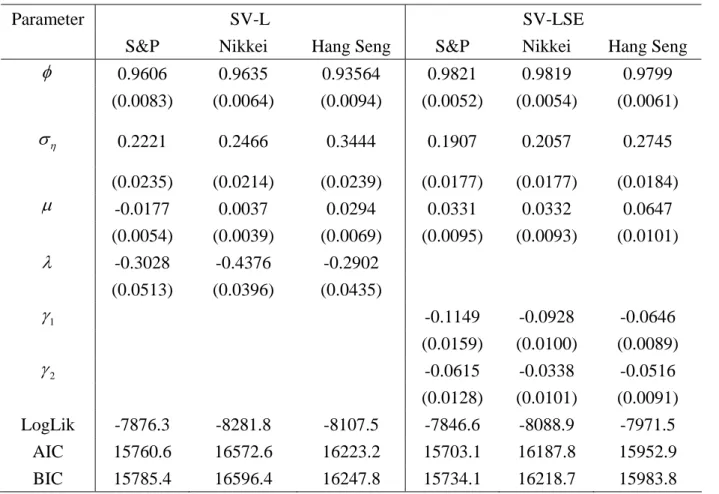
.Table 1 shows the MCL estimates of the univariate SV-L and SV-LSE models. All
the estimated parameters are significant at the five percent level, except for µ in the
SV-L model for Nikkei. As Table 1 also shows that ρ<0 in the SV-L models and
1 2 0
γ <γ < in the SV-LSE model, there exist clear leverage effects in all three data sets.
The SV-L and SV-LSE models are estimated by using the MCL method based on the
distribution of lnyt2. For all data sets, the SV-LSE model is preferred to the SV-L
model on the basis of AIC and BIC.
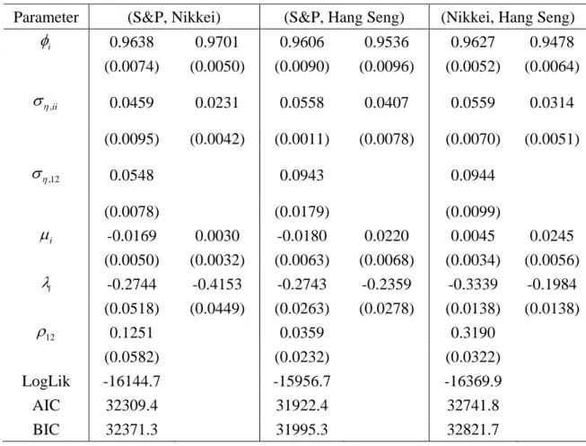
Table 2 presents the estimates of the bivariate SV-L model. For each pair of three
data sets, all the estimates of ση,12, which is the parameter of the instantaneous
correlation of volatility, are significant at the five percent level. While the correlation
between the variables, ρ12, is significant for the pairs (S&P, Nikkei) and (Nikkei, Hang
Seng), it is insignificant for the pair (S&P, Hang Seng). The significance (and insignificance) and signs of the estimates of the other parameters are unchanged from the univariate case in Table 1.
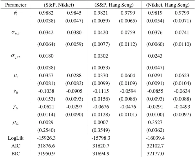
For the bivariate SV-LSE model, the MCL estimates in Table 3 indicate that the
estimates of ση,12 and ρ12 are significant for all three pairs of variables, which
AIC and BIC in Table 3 for SV-LSE with those in Table 2 for SV-L, the bivariate SV-L model is preferred for all data sets. The results in Tables 1-3 also indicate the likelihood
ratio tests for the null hypothesis ση,ij =ρij =0 for any , (i j i≠ j) reject the
univariate models in favour of their bivariate counterparts.
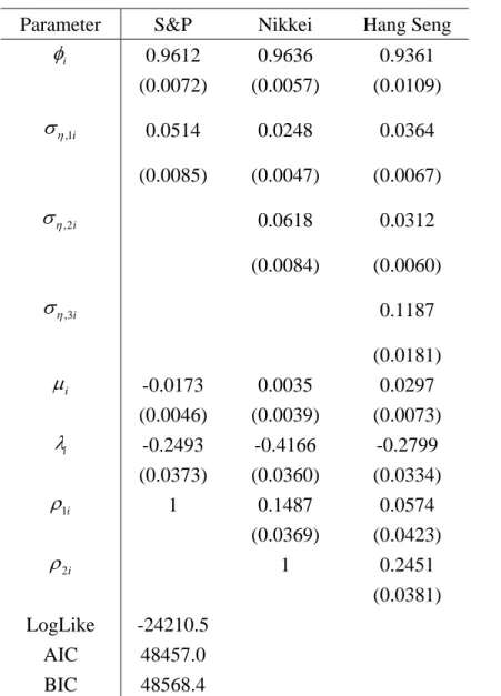
Table 4 shows the results for the trivariate SV-L model. All the estimated
off-diagonal elements of Ση and Pε are significant at the five percent level, except
for ρ13, which is the correlation between the conditional distributions of S&P and Hang
Seng. This result is consistent with the estimates from the bivariate models. The
significance of the estimated off-diagonal elements of Ση and Pε implies the
rejection of the univariate models in favour of the trivariate SV-L model. The signs and significance of the other parameter estimates are unchanged from the univariate case.
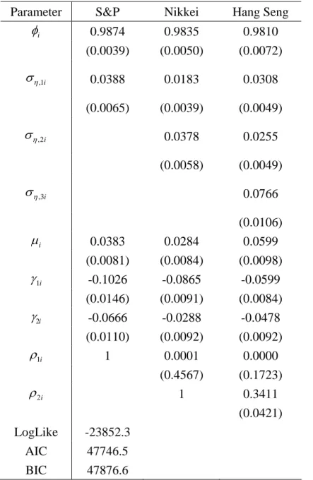
Table 5 presents the MCL estimates for the trivariate SV-LSE model. As all the
estimated off-diagonal elements of Ση and Pε are significant at the five percent level,
this result is also consistent with the estimates from the bivariate models. The
significance of all the off-diagonal elements of Ση and Pε implies the rejection of the
univariate models in favour of the trivariate SV-LSE model. The signs and significance of the other estimated parameter are unchanged from the univariate case.
5 Concluding Remarks
In this paper, two types of asymmetric multivariate stochastic volatility (SV) models were proposed and analysed, namely: (i) “SV with leverage” (SV-L) model based on the negative correlation between the innovations in the returns and volatility; and (ii) “SV with leverage and size effect” (SV-LSE) model based on the signs and magnitude of the returns.
The paper derived the state space form for the logarithm of the squared returns which follow the multivariate SV-L model, and developed estimation methods for the multivariate SV-L and SV-LSE models based on the Monte Carlo likelihood (MCL)
approach. The empirical results showed that the multivariate SV-LSE model fits the data more accurately with respect to AIC and BIC than does the multivariate SV-L model to the bivariate and trivariate returns of S&P 500, Nikkei 225, and Hang Seng indexes. Moreover, the empirical results suggest that the univariate models should be rejected in favour of their bivariate and trivariate counterparts.
The asymmetric multivariate SV-LSE and SV-L models can be extended in terms of distributional considerations, as follows:
(1) Modelling the tails of the conditional distribution: A direct way of accommodating
this problem is to assume the Student t-distribution or a mixture of two or more normal
distributions (for further details, see Liesenfeld and Jung (2000), Bai, Russell and Tiao (2003), and Watanabe and Asai (2003), among others). In this context, we may consider asymmetric multivariate SV models with heavy-tailed distributions.
(2) An alternative is to consider the two factor model analyzed by Chernov et al. (2003). In their specification, the second SV factor is expected to act as a factor dedicated to the exclusive modelling of the tail behaviour. The empirical analysis of Asai (2005) indicates that AIC and BIC tend to select two-factors among multi-factors for S&P 500 and TOPIX stock returns. Based on these results, the asymmetric multivariate and multi-factor SV model would seem to be useful candidates for extension.
Appendix A:
Some Moments of the Folded Normal and Half Normal
Distributions
If X has a normal distribution with mean µ and variance σ2, X N
(
µ σ, 2)
,then Y = X is said to have a folded normal distribution. Leone, Nelson and
Nottingham (1961) discussed various properties and applications of the folded normal distribution, while Elandt (1961) derived the general formula for the moments. The first and second moments are given by
( )
( )
2 2 2 2 2 2 exp 1 2 , 2 , E Y E Y µ µ σ µ π σ σ µ σ ⎛ ⎞ ⎡ ⎛ ⎞⎤ = ⎜− ⎟− ⎢ − Φ⎜ ⎟⎥ ⎝ ⎠ ⎣ ⎦ ⎝ ⎠ = +where Φ
( )
x is the distribution function of the standard normal distribution. If thefolding is about the mean, such that µ =0, this leads to a half normaldistribution. The
first and second moments of the half normal distribution are 2 π and σ2 ,
respectively. For odd moments, E Y⎡⎣ 2n+1⎤ =⎦
( )
2n ...6 4 2⋅ ⋅ σ2n+1 2 π(
n=1, 2, 3,K)
.This paper uses the mean of the folded normal distribution, which requires the
derivation of two expectations, namely E⎡⎣Φ
( )
aε ε2⎤⎦ and E⎡⎣Φ( )
aε ε lnε2⎤⎦ ,where a is a constant and ε follows a half normal distribution with unit variance.
In order to derive these expectations, it is convenient to use the power series of
( )
z( )
( )
2(
1)
0 1 , 2 1 3 5 2 1 n n z z z n φ ∞ + = Φ = + ⋅ ⋅ +∑
Kwhere φ
( )
z is the standard normal density function (see Abramowitz and Stegun(1970, Section 26.2.11)). Substituting the power series into the above expectations leads to the following:
( )
2(
1)
( )
2 3 2 0 1 2 1 3 5 2 1 n n n a E a E a n ε ε ∞ + φ ε ε + = ⎡ ⎤ ⎡Φ ⎤= + ⎣ ⎦∑
⋅ ⋅ K + ⎣ ⎦,( )
2(
1)
( )
2 2 2 2 2 0 1 ln ln ln , 2 1 3 5 2 1 n n n a E a E E a n ε ε ε ε ε ∞ + φ ε ε + ε = ⎡ ⎤ ⎡Φ ⎤= ⎡⎣ ⎤⎦+ ⎣ ⎦∑
⋅ ⋅ K + ⎣ ⎦as it is possible to exchange the summation and integral for these cases. Based on the odd moments of the half normal distribution, we have
( )
2 2 1(
2)
3/ 2(
(
)
)
0 2 4 6 2 2 1 1 1 3 5 2 1 n n n n E a a a n ε ε π ∞ − − + = ⋅ ⋅ + ⎡Φ ⎤= + ⎣ ⎦∑
⋅ ⋅ KK + .In order to obtain an analytical solution of the above expression, the expectations of the chi-squared distribution and a property of the gamma function are required, namely:
[
]
2 2 2 ln ln E ε ε E χ π ⎡ ⎤ = ⎣ ⎦ ,(
)
( )
[
]
1 1 2 2 2 1 2 ln ln 2 n n n n E χν χν ν E χ ν ν + + + + Γ + + ⎡ ⎤ = ⎣ ⎦ Γ ,According to Abramowitz and Stegun (1970, Section 26.4.36),
[
ln]
( )
2 ln 2E χν =ψ ν + , where ψ
( )
is the digamma function, which leads to thefollowing:
( )
{
( )
}
(
)
(
)
{
(
)
}
1/ 2 2 2 3/ 2 2 1 2 0 1 ln 1 ln 2 1 2 1 n 3 2 ln 2 . n n E a a a a a n ε ε ε ψ π ψ − ∞ − − + = ⎡ ⎡Φ ⎤= + + + ⎣ ⎦ ⎢⎣ ⎤ +∑
+ + + ⎥⎦Appendix B. Moments of the Multivariate Half Normal Distribution
In order to consider the multivariate half normal distribution, consider anm-dimensional random vector, X , which follows a multivariate normal distribution
with mean zero and correlation matrix given by P=
{ }
ρij . As X N(
0,P)
, X issaid to have a multivariate half normal distribution. It is straightforward to extend this result to a more general covariance matrix. The purpose of this Appendix is to derive the
first two moments of X and the expectation of the outer-product of X and lnX2.
First, consider a cross-product of the elements of X. For i≠ j, we have
(
|)
i j i j i
E x x = ⎣E x E x⎡ x ⎤⎦.
Noting that xj|xi N
(
ρijxi,1−ρij2)
and xj |xi has the folded normal distribution,we obtain the moments of x xi j as follows:
(
2)
3/ 2(
)
2 2 1 1 2 i j ij i i E x x a ρ E a x x π − ⎡ ⎤ ⎡ ⎤ = + − ⎣ − ⎣Φ ⎦⎦where a=ρij 1−ρij2 . Appendix A shows the closed-form solution of the last
expectation, and also the first two moments of xi . Therefore, we have the first two
moments of the multivariate half normal distribution as
2
, X ,
E X ι E XX P
π ′
= =
where the
( )
i i, element of PX is one, while the( )
i j, element is given by(
2)
3/ 2 2 2(
(
)
)
0 2 4 6 2 2 2 1 1 1 3 5 2 1 n ij ij n n n ρ ρ π ∞ + = ⎡ ⋅ ⋅ + ⎤ − ⎢ + ⎥ ⋅ ⋅ + ⎣∑
⎦ K K .Now consider the expectation of the outer product of X and lnX2, that is,
{
2}
ln X
R ≡ ⎢E X⎡ X ′⎤⎥
⎣ ⎦ . For the univariate standard normal variable x , where
( )
0,1x N , Harvey and Shephard (1996) showed that
(
2)
{
( )
}
ln 1 2 ln 2 2
E x x = ψ + π .
Thus, the
( )
i i, element of RX is{
ψ( )
1 2 +ln 2}
2 π , so that it is only necessaryto consider the off-diagonal elements of RX , E x⎡⎣ i lnx2j⎤⎦. As the expectation of
|
i j
(
)
( )
2 2 1/ 2 2 2 2 2 2 ln | ln 2 1 1 exp ln 2 1 2 ln 2 2 ln . 2 i j i j j j j ij j j j E x x E E x x x a E a x x E a x x x π ρ ψ π − ⎡ ⎤ ⎡ ⎤= ⎡⎣ ⎤⎦ ⎣ ⎦ ⎣ ⎦ ⎡ ⎛ ⎞ ⎤ = + ⎢ ⎜− ⎟ ⎥ ⎝ ⎠ ⎣ ⎦ ⎡⎧ ⎛ ⎞ ⎫ ⎡ ⎤⎤ − ⎢⎨ ⎜ ⎟+ ⎬ − ⎣Φ ⎦⎥ ⎝ ⎠ ⎩ ⎭ ⎣ ⎦For the right-hand side, we can derive the solution of the first term by tedious
calculation, while the last term is given in Appendix A. Therefore, the
( )
i j, element ofX R is give by
(
2) (
2)
2 0 2 2 1 ln 1 1 ln 2 2 n ij ij ij n n ρ ρ ρ ψ π ∞ = ⎡ − + − ⎧ ⎛ + ⎞+ ⎫⎤ ⎨ ⎬ ⎢ ⎜⎝ ⎟⎠ ⎥ ⎩ ⎭ ⎣∑
⎦.Appendix C. Moments of the Transformed Leverage MSV Model
The logarithmic transformation of the Leverage MSV model yields the state space
form of equations (10) and (11), which will be developed in this Appendix. Let Es
denote the expectation conditional on the signs of yt, st, and assign a similar
interpretation to the respective variance and covariance operators. Recalling the fact that
(
1 1)
| ,
t t N LPε t η LP Lε
η ε −ε Σ − −
and the results of Appendix B, we have
[
]
1 2 1 ( ) ( | ) , t Es t E Es t t Es LPε t LP sε t µ η η ε ε π ∗≡ = = ⎡ − ⎤= − ⎣ ⎦[
]
, 1 1 1 1 1 1 1 1 1 1 ( ) ( ) ( ) ( ) 2 ( | ) 2 ( ) 2 ( ) , t s t s t t s t s t s t t t t t s t t t t t t V E E E E E LP s s P L LP L LP E P L LP s s P L LP L LP P s s P L η ε ε η ε ε ε ε ε η ε ε ε ε η η η η η η η ε π ε ε π ιι π ∗ − − − − − − − − − − ′ ′ Σ ≡ = − ′ ′ = − ′ ′ = Σ − + − ⎡⎧ ′⎫ ′ ⎤ = Σ − + ⎢⎨ − ⎬ ⎥ ⎩ ⎭ ⎣ o ⎦ and{ }
( )
{ }
(
)
{ }
{ }
2 2 2 1 1 2 1 ( , ) ln ln 2 | ln 2 ln 2 ( ) , t s t t s t t s t t s t t t t s t t t t L Cov E E E E E c LP s LP E c s LP R c s ε ε ε ε η ξ η ε η ε η ε ε ι π ε ε ι π ι π ∗ − − − ⎡ ′⎤ ⎛ ′⎞ ≡ = ⎢ ⎥− ⎜ ⎟ ⎣ ⎦ ⎝ ⎠ ⎡ ′⎤ ′ = ⎢ ⎥− ⎣ ⎦ ⎡ ⎡ ′⎤ ⎤ ′ = ⎢ ⎢ ⎥− ⎥ ⎣ ⎦ ⎣ ⎦ ⎡⎧⎪ ⎫⎪ ⎤ ′ = ⎢⎨ − ⎬ ⎥ ⎪ ⎪ ⎢⎩ ⎭ ⎥ ⎣ o ⎦where Pε and Rε are the correlation matrices of the multivariate half normal
distribution arising from εt N
(
0,Pε)
and the expectation of the outer-product oft
ε and lnεt2 , respectively. The constant c is defined by
( )
1 2 ln 2 1.2703References
Abramowitz, M. and N. Stegun (1970), Handbook of Mathematical Functions, Dover
Publications, NY.
Asai, M. (2005), “Autoregressive Stochastic Volatility Models with Heavy-Tailed Distribution: A Comparison with Multi-Factor Volatility Models”, unpublished paper, Faculty of Economics, Soka University.
Asai, M. and M. McAleer (2005a), “Dynamic Asymmetric Leverage in Stochastic
Volatility Models”, Econometric Reviews, 24, 317-332.
Asai, M. and M. McAleer (2005b), “Alternative Leverage and Threshold Effects in Stochastic Volatility Models”, unpublished paper, Faculty of Economics, Soka University.
Bai, X., J.R. Russell and G.C. Tiao (2003), “Kurtosis of GARCH and Stochastic
Volatility Models with Non-normal Innovations,” Journal of Econometrics, 114,
349-360.
Bollerslev, T., R.F. Engle and J. Wooldridge (1988), “A Capital Asset Pricing Model
with Time Varying Covariances”, Journal of Political Economy, 96, 116–131.
Chernov, M., A.R. Gallant, E. Ghysels and G. Tauchen (2003), “Alternative Models for
Stock Price Dynamics”, Journal of Econometrics, 116, 225-257.
Chesney, M. and L.O. Scott (1989), “Pricing European Currency Options: A Comparison of the Modified Black-Scholes Model and a Random Variance Model”,
Journal of Financial and Quantitative Analysis, 24, 267-284.
Christie, A.A. (1982), “The Stochastic Behavior of Common Stock Variances: Value,
Leverage and Interest Rate Effects”, Journal of Financial Economics, 10, 407-432.
Danielsson, J. (1994), “Stochastic Volatility in Asset Prices: Estimation with Simulated
Danielsson, J. (1998), “Multivariate Stochastic Volatility Models: Estimation and a
Comparison with VGARCH Models”, Journal of Empirical Finance, 5, 155–173.
Durbin, J. and S.J. Koopman (1997), “Monte Carlo Maximum Likelihood Estimation
for Non-Gaussian State Space Models”, Biometrika, 84, 669-684.
Elandt (1961), “The Folded Normal Distribution: Two Methods of Estimating
Parameters from Moments,” Technometrics, 3, 551-562.
Gallant, A.R. and G. Tauchen (1996), “Which Moments to Match?”, Econometric
Theory, 12, 657–681.
Glosten, L., R. Jagannathan and D. Runkle (1992), “On the Relation Between the
Expected Value and Volatility of Nominal Excess Returns on Stocks”, Journal of
Finance, 46, 1779-1801.
Harvey, A.C., E. Ruiz and N. Shephard (1994), “Multivariate Stochastic Variance
Models”, Review of Economic Studies, 61, 247-264.
Harvey, A.C. and N. Shephard (1996), “Estimation of an Asymmetric Stochastic
Volatility Model for Asset Returns”, Journal of Business and Economic Statistics, 14,
429-434.
Higham, N.J. (1988), “Computing a Nearest Symmetric Positive Semidefinite Matrix”,
Linear Algebra and its Applications, 103, 103-118.
Hull, J. and A. White (1987), “The Pricing of Options on Assets with Stochastic
Volatility”, Journal of Finance, 42, 281-300.
Jacquier, E., N.G. Polson and P.E. Rossi (1994), “Bayesian Analysis of Stochastic
Volatility Models”, Journal of Business and Economic Statistics, 12, 371-389.
Jacquier, E., N.G. Polson and P.E. Rossi (2004), “Bayesian Analysis of Stochastic
Volatility Models with Fat-tails and Correlated Errors”, Journal of Econometrics, 122,
Koopman, S.J. and E.H. Uspensky (2002), “The Stochastic Volatility in Mean Model:
Empirical Evidence from International Stock Markets”, Journal of Applied
Econometrics, 17, 667-689.
Leone, F.C., L.S. Nelson and R.B. Nottingham (1961), “The Folded Normal
Distribution,” Technometrics, 3, 543-550.
Liesenfeld, R. and R.C. Jung (2000), “Stochastic Volatility Models: Conditional
Normality Versus Heavy-Tailed Distributions,” Journal of Applied Econometrics, 15,
137-160.
Liesenfeld, R. and J.-F. Richard (2003), “Univariate and Multivariate Stochastic
Volatility Models: Estimation and Diagnostics”, Journal of Empirical Finance, 10,
505-531.
McAleer, M. (2005), “Automated Inference and Learning in Modeling Financial
Volatility”, Econometric Theory, 21, 232-261.
Nelson, D.B. (1991), “Conditional Heteroskedasticity in Asset Returns: A New
Approach”, Econometrica, 59, 347-370.
Sandmann, G. and S.J. Koopman (1998), “Estimation of Stochastic Volatility Models
via Monte Carlo Maximum Likelihood”, Journal of Econometrics, 87, 271-301.
Shephard, N. (1996), “Statistical Aspects of ARCH and Stochastic Volatility”, in D.R.
Cox, D.V. Hinkley and O.E. Barndorff-Nielsen (eds.), Time Series Models in
Econometrics, Finance and Other Fields, Chapman & Hall, London, pp. 1-67.
So, M.K.P., W.K. Li and K. Lam (2002), “A Threshold Stochastic Volatility Model”,
Journal of Forecasting, 21, 473-500.
Taylor, S.J. (1986), Modelling Financial Time Series, Wiley, Chichester.
Watanabe, T. and M. Asai (2003), “Stochastic Volatility Models with Heavy-Tailed Distributions: A Bayesian Analysis,” unpublished paper, Faculty of Economics, Tokyo Metropolitan University.
Wiggins, J.B. (1987), “Option Values Under Stochastic Volatility: Theory and
Empirical Estimates”, Journal of Financial Economics, 19, 351-372.
Yu, J. (2005), “On Leverage in a Stochastic Volatility Model”, Journal of Econometrics,
Table 1: MCL Estimates of the Univariate SV-L and SV-LSE Models
Parameter SV-L SV-LSE
S&P Nikkei Hang Seng S&P Nikkei Hang Seng
φ 0.9606 0.9635 0.93564 0.9821 0.9819 0.9799 (0.0083) (0.0064) (0.0094) (0.0052) (0.0054) (0.0061) η σ 0.2221 0.2466 0.3444 0.1907 0.2057 0.2745 (0.0235) (0.0214) (0.0239) (0.0177) (0.0177) (0.0184) µ -0.0177 0.0037 0.0294 0.0331 0.0332 0.0647 (0.0054) (0.0039) (0.0069) (0.0095) (0.0093) (0.0101) λ -0.3028 -0.4376 -0.2902 (0.0513) (0.0396) (0.0435) 1 γ -0.1149 -0.0928 -0.0646 (0.0159) (0.0100) (0.0089) 2 γ -0.0615 -0.0338 -0.0516 (0.0128) (0.0101) (0.0091) LogLik -7876.3 -8281.8 -8107.5 -7846.6 -8088.9 -7971.5 AIC 15760.6 16572.6 16223.2 15703.1 16187.8 15952.9 BIC 15785.4 16596.4 16247.8 15734.1 16218.7 15983.8
Note: ‘LogLik’ is the log-likelihood based on lnyt2, and AIC and BIC are calculated based on
Table 2: MCL Estimates for the Bivariate SV-L Model
Parameter (S&P, Nikkei) (S&P, Hang Seng) (Nikkei, Hang Seng)
i φ 0.9638 0.9701 0.9606 0.9536 0.9627 0.9478 (0.0074) (0.0050) (0.0090) (0.0096) (0.0052) (0.0064) ,ii η σ 0.0459 0.0231 0.0558 0.0407 0.0559 0.0314 (0.0095) (0.0042) (0.0011) (0.0078) (0.0070) (0.0051) ,12 η σ 0.0548 0.0943 0.0944 (0.0078) (0.0179) (0.0099) i µ -0.0169 0.0030 -0.0180 0.0220 0.0045 0.0245 (0.0050) (0.0032) (0.0063) (0.0068) (0.0034) (0.0056) i λ -0.2744 -0.4153 -0.2743 -0.2359 -0.3339 -0.1984 (0.0518) (0.0449) (0.0263) (0.0278) (0.0138) (0.0138) 12 ρ 0.1251 0.0359 0.3190 (0.0582) (0.0232) (0.0322) LogLik -16144.7 -15956.7 -16369.9 AIC 32309.4 31922.4 32741.8 BIC 32371.3 31995.3 32821.7
Note: ‘LogLik’ is the log-likelihood based on lnyt2, and AIC and BIC are calculated
Table 3: MCL Estimates for the Bivariate SV-LSE Model
Parameter (S&P, Nikkei) (S&P, Hang Seng) (Nikkei, Hang Seng)
i φ 0.9882 0.9845 0.9821 0.9799 0.9819 0.9799 (0.0038) (0.0047) (0.0059) (0.0065) (0.0054) (0.0071) ,ii η σ 0.0342 0.0380 0.0420 0.0759 0.0376 0.0741 (0.0064) (0.0059) (0.0077) (0.0112) (0.0060) (0.0110) ,12 η σ 0.0180 0.0302 0.0243 (0.0038) (0.0053) (0.0047) i µ 0.0357 0.0288 0.0370 0.0604 0.0291 0.0623 (0.0081) (0.0083) (0.0099) (0.0109) (0.0091) (0.0104) 1i γ -0.1038 -0.0905 -0.1115 -0.0594 -0.0855 -0.0634 (0.0153) (0.0093) (0.0156) (0.0086) (0.0093) (0.0088) 2i γ -0.0621 -0.0297 -0.0676 -0.0476 -0.0291 -0.0493 (0.0114) (0.0090) (0.0128) (0.0101) (0.0100) (0.0097) 12 ρ 0.0029 0.0007 0.3527 (0.2540) (0.3549) (0.0362) LogLik -15926.3 -15798.3 -16039.4 AIC 31876.6 31620.7 32102.7 BIC 31950.9 31694.9 32177.0
Note: ‘LogLik’ is the log-likelihood based on lnyt2, and AIC and BIC are calculated based
Table 4: MCL Estimates for the Trivariate SV-L Model
Parameter S&P Nikkei Hang Seng
i φ 0.9612 0.9636 0.9361 (0.0072) (0.0057) (0.0109) ,1i η σ 0.0514 0.0248 0.0364 (0.0085) (0.0047) (0.0067) ,2i η σ 0.0618 0.0312 (0.0084) (0.0060) ,3i η σ 0.1187 (0.0181) i µ -0.0173 0.0035 0.0297 (0.0046) (0.0039) (0.0073) i λ -0.2493 -0.4166 -0.2799 (0.0373) (0.0360) (0.0334) 1i ρ 1 0.1487 0.0574 (0.0369) (0.0423) 2i ρ 1 0.2451 (0.0381) LogLike -24210.5 AIC 48457.0 BIC 48568.4
Note: ‘LogLik’ is the log-likelihood based on lnyt2, and
Table 5: MCL Estimates for the Trivariate SV-LSE Model
Parameter S&P Nikkei Hang Seng
i φ 0.9874 0.9835 0.9810 (0.0039) (0.0050) (0.0072) ,1i η σ 0.0388 0.0183 0.0308 (0.0065) (0.0039) (0.0049) ,2i η σ 0.0378 0.0255 (0.0058) (0.0049) ,3i η σ 0.0766 (0.0106) i µ 0.0383 0.0284 0.0599 (0.0081) (0.0084) (0.0098) 1i γ -0.1026 -0.0865 -0.0599 (0.0146) (0.0091) (0.0084) 2i γ -0.0666 -0.0288 -0.0478 (0.0110) (0.0092) (0.0092) 1i ρ 1 0.0001 0.0000 (0.4567) (0.1723) 2i ρ 1 0.3411 (0.0421) LogLike -23852.3 AIC 47746.5 BIC 47876.6
Note: ‘LogLik’ is the log-likelihood based on lnyt2, and