C A R F W o r k i n g P a p e r
CARF is presently supported by Bank of Tokyo-Mitsubishi UFJ, Ltd., Citigroup, Dai-ichi Mutual Life Insurance Company, Meiji Yasuda Life Insurance Company, Nippon Life Insurance Company, Nomura Holdings, Inc. and Sumitomo Mitsui Banking Corporation (in alphabetical order). This financial support enables us to issue CARF Working Papers.
CARF Working Papers can be downloaded without charge from: http://www.carf.e.u-tokyo.ac.jp/workingpaper/index.cgi
Working Papers are a series of manuscripts in their draft form. They are not intended for circulation or distribution except as indicated by the author. For that reason Working Papers may not be reproduced or distributed without the written consent of the author.
CARF-F-177
Pricing Average Options on Commodities
Kenichiro Shiraya
Mizuho-DL Financial Technology Co.,Ltd. Akihiko Takahashi
The University of Tokyo First Version: October 2009 Current Version: February 2012
Pricing Average Options on Commodities
1Kenichiro Shiraya2, Akihiko Takahashi 3 February 11, 2012
1We are very grateful to the editor, Professor Robert Webb and an anonymous referee for
their efforts and precious comments.
2Kenichiro Shiraya is a Senior Financial Engineer at Mizuho-DL Financial Technology Co.,
Ltd., Chiyoda-ku, Tokyo, Japan. Ote Center Building 16F,1-3 Otemachi 1-chome, Chiyoda-ku, Tokyo, Japan. Tel: 81-3-5219-2396, e-mail: kenichiro-shiraya@fintec.co.jp. The views expressed in this paper are those of the author and do not necessarily represent the views of Mizuho-DL Financial Technology Co., Ltd.
3Akihiko Takahashi is a Professor at the Graduate School of Economics, University of Tokyo,
Abstract
This paper proposes a new approximation formula for pricing average options on com-modities under a stochastic volatility environment. In particular, it derives an option pricing formula under Heston and an extended λ-SABR stochastic volatility models (which includes an extended SABR model as a special case). Moreover, numerical examples support the accuracy of the proposed average option pricing formula.
1
Introduction
Average options are very popular derivatives in over-the-counter (OTC) commodity markets. 1 On the contrary, analytic approximation formulas for pricing average price commodity options are unknown except for the Black-Scholes model.
It is fairly common in market practice to price exotic options based on calibration to option prices in a more liquid market (e.g. see pp.48-49 in [1]). For instance, average price options on West Texas Intermediate (WTI) crude oil futures contracts are evaluated based on a model whose parameters are obtained by calibration to the prices of the more liquid American vanilla options on WTI futures traded on the NYMEX division of the CME Group.
However, it is almost impossible for one parameter set under the Black-Scholes op-tion pricing model to reproduce market prices with various strikes for a given maturity. Hence, it is well-known in practice that the Black-Scholes option pricing model is not appropriate for valuation of average price options with calibration to the prices of more liquid plain-vanilla options (e.g. see p.1 in [2]), and that more complex models such as stochastic volatility models are necessary for the calibration.
This paper applies stochastic volatility models and proposes a new approximation formula for pricing average option under Heston model as well as an extension of the λ-SABR (SABR) model (Labordere [11] (Haganet. al.[7])). To the best of our knowledge, this paper is the first one that provides an analytic (approximation) formula under a stochastic volatility environment for the valuation of average options traded in the commodity markets. Moreover, it gives estimates of average option prices under stochastic volatility markets based on the parameters obtained by calibration to the market prices of American options on WTI futures under stochastic volatility models. In addition, our pricing models take the specific feature of the WTI average price option into consideration: the underlying price of an average option is the average of the settlement prices of the first nearby WTI futures contract during the last one month prior to the maturity of the average option. Note also that the expiration of an average option is the last business day of a calendar month, while trading of a WTI futures contract usually ceases on the third business day prior to the twenty-fifth calendar day. Hence, the settlement prices of WTI futures contracts with two consecutive maturities are relevant for the the underlying price of the average option. (See (2) in Section 2.) Similarly, American options on WTI futures with two consecutive maturities are relevant for calibration to plain-vanilla option prices. The proposed models in this paper incorporate those features of the WTI average price option.
Although Yoshida [24] and Takahashi[13],[14] apply the asymptotic expansion method to pricing average options, the underlying price they consider is a continuous average of an asset price that does not represent the underlying price of a contract in the real world precisely. Hence the formula they derived can not be used directly for valuation of average options traded in actual markets. Also they do not investigate the numerical
1
Average options are traded mainly in OTC markets (e.g. see P.40 in [9]), while they are illiquid in the listed markets such as CME Group.
accuracies of the third order expansion under stochastic volatility models.
As for pricing average options with stochastic volatility models, there are some exiting works: for instance, Fouque and Han[4] have derived asymptotic solutions to arithmetic average options under a class of fast mean-reverting stochastic volatility models. Wong and Cheung[22] extended their works to geometric average options pricing and calibration. Fouque and Han[5] used the solution of Wong and Cheung[22] to construct an efficient simulation method for arithmetic average options. Although these works did not consider the types of options in this paper directly, their methods may be applicable to the product considered here.
This paper takes Heston model(Heston [8]) and the extendedλ-SABR model that includes the extended SABR model as a special case: They are very popular models for calibration to plain-vanilla option prices in the various markets. Numerical experiments show the sufficient accuracies of our approximation formulas for pricing average options under those stochastic volatility models. Moreover, calibration to the market prices of American options on WTI futures are implemented and average option prices in the WTI market are estimated based on the calibrated parameters.
Note that it is not efficient in numerical computation to calibrate directly to the American options under a stochastic volatility model. Alternatively, an implied volatil-ity for each strike and maturvolatil-ity is estimated from a market price of the American option under a binomial version of Black-Scholes model. Then, the corresponding European option price is computed with its implied volatility. Next, given a maturity, calibra-tion is implemented against those European prices with different strikes simultaneously under Heston, SABR and λ-SABR models. 2 Especially, vanilla option prices under λ-SABR model are computed by the third order expansion formula of the asymptotic method, which makes calibration very efficient.
Finally, the prices of average options traded in the WTI market are evaluated with the calibrated parameters by the asymptotic expansion formula as well as Monte Carlo simulations. Further, those estimated prices are compared with the settlement prices of average options traded in CME Group. Note that average options in CME Group are illiquid since they are traded mainly in OTC market. However, there are no official prices in the OTC market, while the settlement prices in CME Group are announced every day for the contracts with positive open interests. Thus, the settlement prices of average options are used as the reference prices in our study.
The organization of the paper is as follows: The next section briefly explains the structures of average options traded in commodity markets and then describes the extended λ-SABR and Heston models. Section 3 derives a new asymptotic expansion formula for the average options. Section 4 presents series of numerical experiments. Section 5 concludes. Appendix summarizes formulas of the conditional expectations used for the asymptotic expansion up to the third order.
2
Average Options under Stochastic Volatility Models
This section briefly describes the structure of average options on commodities, where the underlying assets are the averages of spot prices or future prices. Then, it presents two stochastic volatility models, an extended λ-SABR model and Heston model ([8]) used in the subsequent analysis: the extended λ-SABR model adds a drift term to the original model introduced by [11]. Note that the model with λ = 0 is reduced to the extended SABR model. (The original SABR model is introduced by [7].)
2.1 Average Option on Commodities
The underlying asset price of an average option contract on commodities is the average of settlement prices from the first business day to the last business day of a calendar month. In addition, there are two standard types of contracts.
One type is mostly applied to average options on metals in OTC markets(e.g. Copper). It calculates an average of a commodity’s spot-price every business day through the month. Let the reference dates t1,· · ·, tn (t1 < · · · < tn = T), and the spot priceS. Then, the underlying asset’s price of this type is expressed as follows:
X(T) = 1 n ( n ∑ i=1 S(ti) ) . (1)
Another standard type is mainly traded in OTC oil markets(e.g. WTI). It refers to a futures price every business day. As the expiration of trading a futures contract is about a week before the end of a calendar month, the futures contracts with two consecutive maturities become the underlying assets of an average option. More precisely, let the reference dates t1,· · ·, tn1 for the first contract and t′1,· · · , t′n2 for the subsequent contract (t1<· · ·< tn1 < t1′ <· · ·< t′n2 =T). Also denote the relevant two underlying futures prices asSi,i= 1,2. Then, the average price of this type is expressed as follows:
X(T) = 1 n1+n2 (n 1 ∑ i=1 S1(ti) + n2 ∑ i=1 S2(t′i) ) . (2)
Thus, the payoff functions of average call and put options with strike priceK and maturity T are given by max{X(T)−K,0} and max{K−X(T),0}, respectively.
The subsequent sections will concentrate on the second type because it includes the first type as a special case in terms of the way of averaging. However, there is a difference in the underlying asset, a spot or futures. In order that the difference does not cause any problems, this paper will present the underlying assets’ models and pricing formulas which can be applied to both types.
Moreover, it is common in practice that pricing an average option is based on the calibration to the prices of the liquid vanilla options whose underlying assets are the same spot or futures contracts as those of the average option. Hence, in order for calibration, this paper will apply stochastic volatility models to the underlying assets’ dynamics.
2.2 Stochastic Volatility Models
We take an extendedλ-SABR model and Heston model as the underlying asset model. As remarked before, the extended λ-SABR model becomes the extended SABR model when λ= 0.
First, the extendedλ-SABR model is described. For an average option on a com-modity, the dynamics of the related two underlying asset prices Si (i= 1,2) are de-scribed under the equivalent martingale measure as follows:
dS1(t) = α1(t)S1(t)dt+v1σ1(t)S1(t)β1dZ1(t), (3) dS2(t) = α2(t)S2(t)dt+v2σ2(t)S2(t)β2dZ2(t), (4) dσ1(t) = λ1(θ1−σ1(t))dt+ν1σ1(t)dZ3(t), (5) dσ2(t) = λ2(θ2−σ2(t))dt+ν2σ2(t)dZ3(t), (6) where αi,βi ∈[0,1], λi >0, θi >0 and νi >0 (i= 1,2) are constants, and Z1, Z2, Z3 are correlated Brownian motions with correlations ρ12, ρ23, ρ31∈[−1,1].
Note that Brownian motionZ3driving a stochastic volatility componentσi(i= 1,2) is common for two assets while the correlation (ρ13 or ρ23) between the underlying asset price Si(i = 1,2) and its volatility σi(i = 1,2) is allowed to be different for each asset. Moreover, positive constants v1 and v2 represent different levels of two assets’ volatilities. When the underlying assets are futures contracts, the prices are martingales under the equivalent martingale measure and hence α1(t) =α2(t) = 0 in the corresponding stochastic differential equations described above.
LetW1, W2, W3 independent Brownian motions. Then, the underlying asset prices’ processes are rewritten as follows:
dS1(t) = α1(t)S1(t)dt+µ1σ1(t)S1(t)β1dW1(t), (7) dS2(t) = α2(t)S1(t)dt+µ2,1σ2(t)S2(t)β2dW1(t) +µ2,2σ2(t)S2(t)β2dW2(t), (8) dσ1(t) = λ1(θ1−σ1(t))dt+ν1,1σ1(t)dW1(t) +ν1,2σ1(t)dW2(t) +ν1,3σ1(t)dW3(t), (9) dσ2(t) = λ2(θ2−σ2(t))dt+ν2,1σ1(t)dW1(t) +ν2,2σ2(t)dW2(t) +ν2,3σ2(t)dW3(t), (10) where µ1 =v1, µ2,1 =v2ρ12, µ2,2 =v2c22:=v2 √ 1−ρ212, ν1,1 =ν1ρ31, ν1,2 =ν1c23:=ν1 (ρ23−ρ31ρ12) c22 , ν1,3 =ν1 √ 1−ρ231−c223, ν2,1 =ν2ρ31, ν2,2 =ν2c23:=ν2 (ρ23−ρ31ρ12) c22 , ν2,3 =ν2 √ 1−ρ231−c223. Remark . SABR and λ-SABR models are introduced by Hagan et. al. [7] and Labor-dere [11], respectively. They are defined as follows:
dF(t) = α(t)F(t)βdZ1(t),
dα(t) = λ(¯λ−α(t))dt+να(t)dZ2(t) (λ-SABR), or
dα(t) = να(t)dZ2(t) (SABR),
with F(0) = F, α(0) = α and dZ1dZ2 = ρdt. The term of “SABR model” stands for “stochastic-αβρ model”. This paper extended these models by adding drifts.
Next, Heston model is described. In the similar manner as above, the dynamics of the underlying asset prices in Heston model under the equivalent martingale measure with Brownian motion Z1, Z2, Z3 is given as follows:
dS1(t) = α1(t)S1(t)dt+v1 √ V1(t)S1(t)dZ1(t), (11) dS2(t) = α2(t)S2(t)dt+v2 √ V2(t)S2(t)dZ2(t), (12) dV1(t) = λ1(θ1−V1(t))dt+ν1 √ V1(t)dZ3(t), (13) dV2(t) = λ2(θ2−V2(t))dt+ν2 √ V2(t)dZ3(t). (14) The expression with independent Brownian motions W1, W2, W3 with the same trans-formation of parameters as the extended λ-SABR are obtained:
dS1(t) = α1(t)S1(t)dt+µ1 √ V1(t)S1(t)dW1(t), (15) dS2(t) = α2(t)S1(t)dt+µ2,1 √ V2(t)S2(t)dW1(t) +µ2,2 √ V2(t)S2(t)dW2(t), (16) dV1(t) = λ1(θ1−V1(t))dt+ν1,1 √ V1(t)dW1(t) +ν1,2 √ V1(t)dW2(t) +ν1,3 √ V1(t)dW3(t), (17) dV2(t) = λ2(θ2−V2(t))dt+ν2,1 √ V2(t)dW1(t) +ν2,2 √ V2(t)dW2(t) +ν2,3 √ V2(t)dW3(t). (18)
3
Approximation Formula of Average Options
This section derives an approximation formula for pricing average options on commodi-ties explained in the previous section. Note that the formula based on an asymptotic expansion approach is general enough to be applied to pricing average options under all multi-dimensional diffusion processes. Specifically, this section presents concrete applications for the extended λ-SABR model and Heston model.
3.1 Approximation Formula for Extended λ-SABR Model
First, for given ϵ ∈ (0,1), the extended λ-SABR model in an asymptotic expansion approach is described as follows:
S1(ϵ)(T) = S1(0) +
∫ T 0
+ϵ ∫ T 0 ¯ µ1σ1(ϵ)(t)S (ϵ) 1 (t)dW1(t), (19) S2(ϵ)(T) = S2(0) + ∫ T 0 α2(t)S2(ϵ)(t)dt +ϵ (∫ T 0 ¯ µ2,1σ(2ϵ)(t)S (ϵ) 2 (t)dW1(t) + ∫ T 0 ¯ µ2,2σ(2ϵ)(t)S2(ϵ)(t)dW2(t) ) , (20) σ(1ϵ)(T) = σ1(0) + ∫ T 0 λ1(θ1−σ(1ϵ)(t))dt +ϵ (∫ T 0 ¯ ν1,1σ1(ϵ)(t)dW1(t) + ∫ T 0 ¯ ν1,2σ1(ϵ)(t)dW2(t) + ∫ T 0 ¯ ν1,3σ1(ϵ)(t)dW3(t) ) , (21) σ(2ϵ)(T) = σ2(0) + ∫ T 0 λ2(θ2−σ(2ϵ)(t))dt +ϵ (∫ T 0 ¯ ν2,1σ2(ϵ)(t)dW1(t) + ∫ T 0 ¯ ν2,2σ2(ϵ)(t)dW2(t) + ∫ T 0 ¯ ν2,3σ2(ϵ)(t)dW3(t) ) , (22) X(ϵ)(T) = 1 n1+n2 (n 1 ∑ i=1 S1(ϵ)(ti) + n2 ∑ i=1 S2(ϵ)(t′i) ) . (23) whereϵµ¯1 = µ1, ϵµ¯2,1 = µ2,1, ϵµ¯2,2 = µ2,2, ϵν¯1 = ν1, ϵν¯2,1 = ν2,1, ϵν¯2,2 = ν2,2. Then, Si(T), σi(T), X(T) is expanded around 0 as
X(ϵ)(T) ≈ X(0)(T) +ϵX(1)(T) +· · · , (24) Si(ϵ)(T) ≈ Si(0)(T) +ϵSi(1)(T) +· · ·, (25) σ(iϵ)(T) ≈ σi(0)(T) +ϵσ(1)i (T) +· · ·, (26) where X(n)(T) := ∂nX∂ϵ(ϵ)n(T)|ϵ=0,Si(n)(T) := ∂ nS(ϵ) i (T) ∂ϵn |ϵ=0,σi(n)(T) := ∂ nσ(ϵ) i (T) ∂ϵn |ϵ=0. Remark . The validity of asymptotic expansions appearing in what follows is justi-fied by Watanabe Theory(Watanabe[20]) in Malliavin calculus. In particular, Theorem 2.3 of Watanabe[20] and its truncated version, Theorem 2.2 of Yoshida[23] provided a justification of asymptotic expansions for generalized Wiener functionals. Subse-quent works such as Takahashi[13],[14], Kunitomo and Takahashi[10] and Takahashi-Yoshida[17],[18] have applied Watanabe theory to finance for pricing derivatives and deriving optimal portfolios as well as hedging portfolios. For more detailed explanation and references, see Takahashi[16].
For example, when the underlying factors are generated by (multi-dimensional) gen-eral diffusion processes, Kunitomo-Takahashi[10] provided a justification of the asymp-totic expansion. See Section 3(pp. 920-931) of the paper. Especially, Theorem 3.3. and Corollary 3.1.(p.925) stated it for the case of average options. Since this paper concentrates on the practical applications of an asymptotic expansion, the details are omitted.
The next proposition provides the first four coefficients in the asymptotic expansion of X(ϵ)(T).
Proposition 3.1. We defineN1 and N2 as
N1(t) = 1t≤t1e ∫t1 0 α1(s)ds+· · ·+ 1 t≤tn1e ∫tn1 0 α1(s)ds, N2(t) = 1t≤t′1e ∫t′1 0 α2(s)ds+· · ·+ 1 t≤t′n2e ∫t′n 2 0 α2(s)ds. Set M =n1+n2 andW(t) = (W1(t), W2(t), W3(t))′. Then,
X(0)(T) = N1(0)S1(0) +N2(0)S2(0) M , (27) X(1)(T) = ∫ T 0 f11(s)′dW(s), (28) X(2)(T) = 2 4 ∑ i=1 ∫ T 0 ∫ s 0 f2i(u)′dW(u)g2i(s)′dW(s), (29) X(3)(T) = 6 ( 6 ∑ i=1 ∫ T 0 ∫ s 0 ∫ u 0 f3i(v)′dW(v)g3i(u)′dW(u)h3i(s)′dW(s) + 4 ∑ i=1 ∫ T 0 (∫ s 0 g4i(u)′dW(u) ) (∫ s 0 f4i(u)′dW(u) ) ×h4i(s)′dW(s) ) . (30)
Also setηi(t) =θi+ (σi(0)−θi)e−λit,ξi(t) =Si(0)e
∫t 0αi(s)ds and then,f 11(t),f2i(t), g2i(t) (i= 1,· · ·,4), f3i(t) ,g3i(t), h3i(t) (i= 1,· · ·,6),f4i,g4i, h4i (i= 1,· · · ,4), are expressed as follows: f11(t) = 1 M N 1(t)¯µ1e− ∫t 0α1(s)dsξβ1 1 (t)η1(t) +N2(t)¯µ2,1e− ∫t 0α2(s)dsξβ2 2 (t)η2(t) N2(t)¯µ2,2e− ∫t 0α2(s)dsξβ2 2 (t)η2(t) 0 , f21(t) =f31(t) =f41(t) =g41(t) =g43(t) = µ¯1e −∫t 0α1(s)dsξβ1 1 (t)η1(t) 0 0 ,
f22(t) =f32(t) =f42(t) =g42(t) =g44(t) = ¯ µ2,1e− ∫t 0α2(s)dsξβ2 2 (t)η2(t) ¯ µ2,2e− ∫t 0α2(s)dsξβ2 2 (t)η2(t) 0 , g33(t) = e−λ1t η1(t) f21(t), g34(t) = e−λ2t η2(t) f22(t), g35(t) = νν¯¯11,,12 ¯ ν1,3 , g36(t) = νν¯¯22,,12 ¯ ν2,3 , f23(t) =f33(t) =f35(t) =f43(t) =η1(t)eλ1tg35(t), f24(t) =f34(t) =f36(t) =f44(t) =η2(t)eλ2tg36(t), g31(t) = µ¯1ξ β1−1 1 (t)β1η1(t) 0 0 , g32(t) = µ¯2,1ξ β2−1 2 (t)β2η2(t) ¯ µ2,2ξ2β2−1(t)β2η2(t) 0 , g21(t) =h31(t) =h33(t) = N1 (t) M g31(t), g22(t) =h32(t) =h34(t) = N2(t) M g32(t), g23(t) =h35(t) = N1 (t) M g33(t), g24(t) =h36(t) = N2(t) M g34(t), h41(t) = 1 2M N1µ¯1ξ β1−2 1 (t)β1(β1−1)η1(t)e ∫t 0α1(s)ds 0 0 , h42(t) = 1 2M N2µ¯2,1ξ2β2−2(t)β2(β2−1)η2(t)e ∫t 0α2(s)ds N2µ¯2,2ξ2β2−2(t)β2(β2−1)η2(t)e ∫t 0α2(s)ds 0 , h43(t) = N 1e−λ1t M η1(t) g31(t), h44(t) = N 2e−λ2t M η2(t) g32(t).
Proof. We will derive X(0)(T),X(1)(T),and X(2)(T) explicitly. and X(3)(T) can be derived in the similar manner.
First, we calculate X(0)(T). X(0)(T) = 1 n1+n2 (n 1 ∑ i=1 S1(0)(ti) + n2 ∑ i=1 S2(0)(t′i) ) , S1(0)(t) = ( ∫ t 0 α1(s)(S1(0)(s) +ϵS1(1)(s) +· · ·)ds +ϵ ∫ t 0 ¯ µ1(σ(0)1 (s) +ϵσ(1)1 (s) +· · ·)(S1(0)(s) +ϵS1(1)(s) +· · ·)β1dW1(s) +O(ϵ2) ) ϵ=0 = ∫ t 0 α1(s)S1(0)(s)ds.
S1(0)(t) can be solved asS1(0)(t) =e∫0tα1(s)dsS1(0), and S(0)
2 is derived in the same way. Then substituting Si(0)(t) for X(0)(T).
Next, we calculate X(1)(T). X(1)(T) = ∂X (ϵ)(T) ∂ϵ ϵ=0 = 1 n1+n2 (n 1 ∑ i=1 ∂S1(ϵ)(ti) ∂ϵ ϵ=0+ n2 ∑ i=1 ∂S2(ϵ)(t′i) ∂ϵ ϵ=0 ) = 1 n1+n2 (n 1 ∑ i=1 S1(1)(ti) + n2 ∑ i=1 S2(1)(t′i) ) , S1(1)(t) = ∂S (ϵ) 1 (t) ∂ϵ ϵ=0 = ( ∫ t 0 α1(s)(S1(1)(s) +ϵS (2) 1 (s) +· · ·)ds + ∫ t 0 ¯ µ1(σ (0) 1 (s) +ϵσ (1) 1 (s) +· · ·)(S (0) 1 (s) +ϵS (1) 1 (s) +· · ·) β1dW 1(s) +ϵ ∫ t 0 ¯ µ1(σ(0)1 (s) +ϵσ (1) 1 (s) +· · ·)β1S1(1)(s)(S (0) 1 (s) +ϵS (1) 1 (s) +· · ·)β1−1dW1(s) +ϵ ∫ t 0 ¯ µ1(σ(1)1 (s) +ϵσ (2) 1 (s) +· · ·)(S (0) 1 (s) +ϵS (1) 1 (s) +· · ·)β1dW1(s) +O(ϵ2) ) ϵ=0 = ∫ t 0 α1(s)S1(1)(s)ds+ ∫ t 0 ¯ µ1σ1(0)(s)S (0) 1 (s)β1dW1(s), σ(0)1 (t) = ( σ1(0) + ∫ t 0 λ1(θ1−(σ(0)1 (s) +ϵσ(1)1 (s) +· · ·))ds +ϵ 3 ∑ i=1 ∫ t 0 ν1,i(σ1(0)(s) +ϵσ (1) 1 (s) +· · ·)dWi(t) +O(ϵ2) ) ϵ=0 = σ1(0) + ∫ t 0 λ1(θ1−σ1(0)(s))ds.
Those equations can be solved by method of variation of constants as: σ(0)1 (t) = θ1+ (σ1(0)−θ1)e−λ1t, S1(1)(t) = ∫ t 0 ¯ µ1σ1(0)(s)e ∫t sα(u)duS(0) 1 (s) β1dW 1(s).
S2(1) is derived in the same way and the coefficientf11 is derived.
In the same way, to calculateX(2)(T), we get the following equations. X(2)(T) = ∂ 2X(ϵ)(T) ∂ϵ2 ϵ=0 = 1 n1+n2 (n 1 ∑ i=1 S1(2)(ti) + n2 ∑ i=1 S2(2)(t′i) ) ,
S1(2)(t) = ∂ 2S(ϵ) 1 (t) ∂ϵ2 ϵ=0 = ∫ t 0 α1(s)S1(2)(s)ds+ 2 ∫ t 0 ¯ µ1β1σ1(0)(s)S1(0)(s)β1−1S1(1)(s)dW1(s) +2 ∫ t 0 ¯ µ1σ(1)1 (s)S (0) 1 (s)β1dW1(s), σ1(1)(t) = ∂σ (ϵ) 1 (t) ∂ϵ ϵ=0 = − ∫ t 0 λ1σ1(1)(s)ds+ 3 ∑ i=1 ∫ t 0 ν1,iσ(0)1 (s)dWi(t). Those equations can be solved again as follows:
σ(1)1 (t) = 3 ∑ i=1 ∫ t 0 ν1,ie−λ1(t−s)σ(0)1 (s)dWi(t), S1(2)(t) = 2 ∫ t 0 ¯ µ1σ1(0)(s)e ∫t sα1(u)duβ1S(0) 1 (s) β1−1 ∫ s u ¯ µ1σ1(0)(u)e ∫s uα1(w)dwS(0) 1 (u) β1dW 1(u)dW1(s) +2 ∫ t 0 ¯ µ1e ∫t sα1(u)duS(0) 1 (s)β1 ( 3 ∑ i=1 ∫ s 0 ν1,ie−λ1(s−u)σ(0)1 (u)dWi(u) ) dW1(s).
S2(2) is derived in the similar manner, again. Then we can derive f2i(t), g2i(t), i = 1,· · ·,4.
The remaining coefficients can be easily derived in the same way, and the details of derivation are omitted.
Let the riskless interest rate r > 0. Then, the asymptotic expansion of the call price of an average option up to the ϵ3-order with maturity dateT and strike price K is given as follows: C(0) = e−rT ( ϵ ( y ∫ ∞ −y n[x; 0,Σ]dx+ ∫ ∞ −y x n[x; 0,Σ]dx ) +ϵ21 2 ∫ ∞ −y E [ X(2)(T)X(1)(T) =x ] n[x; 0,Σ]dx +ϵ3 ( 1 6 ∫ ∞ −y E [ X(3)(T)X(1)(T) =x ] n[x; 0,Σ]dx +1 8E [( X(2)(T) )2 X(1)(T) =y ] n[y; 0,Σ] )) +o(ϵ3),
where y= X(0)(ϵT)−K, Σ =∫0T f11(s)′f11(s)dsand n[x; 0,Σ] = √21πΣexp
(
−x2 2Σ
)
A more concrete approximation of the price is obtained by the application of con-ditional expectation formulas shown in the appendix.
Remark . The convergence of the option price with the asymptotic expansion was guaranteed by Theorem 3.5 and Corollary 3.1 of Kunitomo and Takahashi[10].
Finally, the following theorem summarizes an analytic approximation formula for pricing average options under the extended λ-SABR model.
Theorem 3.2. The asymptotic expansion up to the ϵ3-order of C(0), the price of an average call option at the contract date with maturity dateT and strike priceK is given as follows: C(0) = e−rT [ ϵ { yN ( y √ Σ ) + Σn[y; 0,Σ] } +ϵ2 ∫ ∞ −y C1 H2(x; Σ) Σ2 n[x; 0,Σ]dx +ϵ3 {∫ ∞ −y C2 H3(x; Σ) Σ3 n[x; 0,Σ]dx+C3n[y; 0,Σ] + ( C4 H4(y; Σ) Σ4 +C5 H2(y; Σ) Σ2 +C6 ) n[y; 0,Σ] }] +o(ϵ3), (31) where y = X(0)(ϵT)−K, Σ = ∫0Tf11(s)′f11(s)ds, n[x; 0,Σ] = √21πΣexp ( −x2 2Σ ) and N(x) denotes the standard normal distribution function. Moreover, Hk(x; Σ) denotes k-th order Hermite polynomial:
Hk(x; Σ) := (−Σ)kex 2/2Σ dk dxke− x2/2Σ . For example,H0(x; Σ) = 1,H1(x; Σ) =x, H2(x; Σ) =x2−Σ, H3(x; Σ) =x3−3Σx, H4(x; Σ) =x4−6Σx2+ 3Σ2. Moreover, Σ = ∫ T 0 f11(s)′f11(s)ds, C1 = 4 ∑ i=1 ∫ T 0 f11(s)′g2i(s) ∫ s 0 f11(u)′f2i(u)duds, C2 = 6 ∑ i=1 ∫ T 0 f11(s)′h3i(s) ∫ s 0 f11(u)′g3i(u) ∫ u 0 f11(v)′f3i(v)dvduds + 4 ∑ i=1 ∫ T 0 f11(s)′h4i(s) ∫ s 0 f11(u)′g4i(u)du ∫ s 0 f11(u)′f4i(u)duds, C3 = 4 ∑ i=1 ∫ T 0 f11(s)′h4i(s) ∫ s 0 g4i(u)′f4i(u)duds,
C4 = 1 2 10 ∑ i=1 (∫ T 0 f11(s)′g5i(s) ∫ s 0 f11(s)′f5i(u)duds ) × (∫ T 0 f11(s)′k5i(s) ∫ s 0 f11(s)′h5i(u)duds ) , C5 = 1 2 10 ∑ i=1 (∫ T 0 f11(s)′k5i(s) ∫ s 0 f11(u)′g5i(u) ∫ u 0 f5i(v)′h5i(v)dvduds + ∫ T 0 f11(s)′g5i(s) ∫ s 0 f11(u)′k5i(u) ∫ u 0 f5i(v)′h5i(v)dvduds + ∫ T 0 f11(s)′g5i(s) ∫ s 0 f5i(u)′k5i(u) ∫ u 0 f11(v)′h5i(v)dvduds + ∫ T 0 g5i(s)′k5i(s) ∫ s 0 f11(u)′h5i(u)du ∫ s 0 f11(u)′f5i(u)duds + ∫ T 0 f11(s)′k5i(s) ∫ s 0 g5i(u)′h5i(u) ∫ u 0 f11(v)′f5i(v)dvduds ) , C6 = 1 2 10 ∑ i=1 ∫ T 0 g5i(s)′k5i(s) ∫ s 0 f5i(u)′h5i(u)duds, where f11(t), f2i(t) (i = 1,· · · ,4), f3i(t) (i = 1,· · ·,6), f4i (i = 1,· · ·,4), g2i(t) (i = 1,· · ·,4), g3i(t) (i = 1,· · · ,6), g4i(t) (i = 1,· · ·,4), h3i(t) (i = 1,· · · ,6) and h4i(t) (i= 1,· · · ,4) are defined above and f5i(t), g5i(t), h5i(t), k5i(t) (i= 1,· · · ,10) are given as follows:
f51(t) =h51(t) =f55(t) =f56(t) =f57(t) =f21(t), f52(t) =h52(t) =h55(t) =f58(t) =f59(t) =f22(t), f53(t) =h53(t) =h56(t) =h58(t) =f510(t) =f23(t), f54(t) =h54(t) =h57(t) =h59(t) =h510(t) =f24(t), g51(t) =k51(t) =g55(t) =g56(t) =g57(t) =g21(t), g52(t) =k52(t) = 1 2k55(t) =g58(t) =g59(t) =g22(t), g53(t) =k53(t) = 1 2k56(t) = 1 2k58(t) =g510(t) =g23(t), g54(t) =k54(t) = 1 2k57(t) = 1 2k59(t) = 1 2k510(t) =g24(t).
Remark . The integrals on the right hand side of (31) are evaluated by the following relation: ∫ ∞ −y 1 ΣkHk(x; Σ)n[x; 0,Σ]dx = 1 Σk−1Hk−1(−y; Σ)n[y; 0,Σ] (k≥1).
Remark . A plain-vanilla option of European type is regarded as a special case of an average option. Hence, set n1 = 1,n2 = 0andt1 =T in (23). Then, an approximation
formula for pricing plain-vanilla options with maturity T under the extended model is obtained by application of this theorem.
3.2 Approximation Formula for Heston Model
An approximation formula for Heston model is obtained in a similar manner as above: Only thing to be done is that the coefficients in Theorem 3.2 are changed to the following.
Set ζi(t) =
√
θi+ (Vi(0)−θi)e−λitand for given ϵ ∈ (0,1), set ϵµ¯1 = µ1, ϵµ¯2,1 = µ2,1, ϵµ¯2,2 =µ2,2, ϵ¯ν1=ν1, ϵν¯2,1=ν2,1, ϵ¯ν2,2 =ν2,2 and S1(ϵ)(T) = S1(0) + ∫ T 0 α1(t)S1(ϵ)(t)dt +ϵ ∫ T 0 ¯ µ1 √ V1(ϵ)(t)S1(ϵ)(t)βdW1(t), (32) S2(ϵ)(T) = S2(0) + ∫ T 0 α2(t)S2(ϵ)(t)dt +ϵ (∫ T 0 ¯ µ2,1 √ V2(ϵ)(t)S2(ϵ)(t)βdW1(t) + ∫ T 0 ¯ µ2,2 √ V2(ϵ)(t)S2(ϵ)(t)βdW2(t) ) , (33) V1(ϵ)(T) = V1(0) + ∫ T 0 λ1(θ1−V1(ϵ)(t))dt +ϵ (∫ T 0 ¯ ν1,1 √ V1(ϵ)(t)dW1(t) + ∫ T 0 ¯ ν1,2 √ V1(ϵ)(t)dW2(t) + ∫ T 0 ¯ ν1,3 √ V1(ϵ)(t)dW3(t) ) , (34) V2(ϵ)(T) = V2(0) + ∫ T 0 λ2(θ2−V2(ϵ)(t))dt +ϵ (∫ T 0 ¯ ν2,1 √ V2(ϵ)(t)dW1(t) + ∫ T 0 ¯ ν2,2 √ V2(ϵ)(t)dW2(t) + ∫ T 0 ¯ ν2,3 √ V2(ϵ)(t)dW3(t) ) , (35) X(ϵ)(T) = 1 n1+n2 (n 1 ∑ i=1 S1(ϵ)(ti) + n2 ∑ i=1 S2(ϵ)(t′i) ) . (36) Then, f11(t) = 1 M N1(t)¯µ1S1(0)N2(ζt1)¯(µt) +2,2SN2(0)2(tζ)¯2µ(2t,)1S2(0)ζ2(t) 0 ,
f21(t) =f31(t) =g31(t) =f41(t) = µ¯1ζ01(t) 0 , f22(t) =f32(t) =g32(t) =f42(t) = µµ¯¯22,,21ζζ22((tt)) 0 , g21(t) =h31(t) = 2h33(t) = N1 (t) M S1(0)f21(t), g22(t) =h32(t) = 2h34(t) = N2 (t) M S2(0)f22(t), g35(t) = 1 ζ1(t) νν¯¯11,,12 ¯ ν1,3 , g36(t) = 1 ζ2(t) νν¯¯22,,12 ¯ ν2,3 , f23(t) =f33(t) =f35(t) =g41(t) =f43(t) =g43(t) =ζ12(t)eλ1tg35(t), f24(t) =f34(t) =f36(t) =g42(t) =f44(t) =g44(t) =ζ22(t)eλ2tg36(t), g33(t) = e−λ1t ζ1(t) µ¯01 0 , g34(t) = e−λ2t ζ2(t) µµ¯¯22,,12 0 , g23(t) = 2h35(t) =h41(t) = N1 (t) 2M S1(0)g33(t), g24(t) = 2h36(t) =h42(t) = N2 (t) 2M S2(0)g34(t), h43(t) = − e−λ1t 4ζ12(t)g23, h44(t) = −e−λ2t 4ζ22(t) g24.
f5i(t),g5i(t), h5i(t),k5i(t) (i= 1,· · ·,10) are given as follows: f51(t) =h51(t) =f55(t) =f56(t) =f57(t) =f21(t), f52(t) =h52(t) =h55(t) =f58(t) =f59(t) =f22(t), f53(t) =h53(t) =h56(t) =h58(t) =f510(t) =f23(t), f54(t) =h54(t) =h57(t) =h59(t) =h510(t) =f24(t), g51(t) =k51(t) =g55(t) =g56(t) =g57(t) =g21(t), g52(t) =k52(t) = 1 2k55(t) =g58(t) =g59(t) =g22(t), g53(t) =k53(t) = 1 2k56(t) = 1 2k58(t) =g510(t) =g23(t), g54(t) =k54(t) = 1 2k57(t) = 1 2k59(t) = 1 2k510(t) =g24(t).
4
Numerical Examples
This section examines effectiveness of our approximation formula through numerical examples.
The asymptotic expansion method is applied to the equations (19) - (23) and (32) - (36) with ϵ = 0.0001 for the extended λ-SABR(SABR) model and Heston model, respectively. 3
4.1 Accuracy of the Approximation Formula
This subsection compares the approximate prices with estimated prices by Monte Carlo simulations.
The setup of the numerical experiments is listed as follows: • Benchmark Prices by Monte Carlo Simulations: 4
time steps: 2,500/year number of trials: 10 million
• The underlying asset prices: S1(0) = 96,S2(0) = 106 the riskless interest rate: 0(r= 0),
the drift of the underlying asset prices: 0(α1(t) =α2(t) = 0),
v1 = 1.1, v2 = 0.9, σ1(0) = σ2(0), V1(0) = V2(0), β1 = β2, λ1 = λ2, θ1 = θ2, ν1 =ν2
• The term of the reference to the first contract(S1) is from 0.9 year to 0.96 year, and the term of the reference to the second contract(S2) is from 0.96 year to 1 year for an one year maturity option.
The term of the reference to the first contract(S1) is from 1.9 year to 1.96 year, and the term of the reference to the second contract(S2) is from 1.96 year to 2 year for a two year maturity option.
Then, the terms are equally divided into 15 for the first contract and 10 for the second contract. (n1= 15, n2 = 10,M = (n1+n2) = 25)
• Call option prices with strike prices: K=70,90,100,120,150 • λ-SABR model parameters (Table 1)
Case i is a benchmark case: In particular, σ(0) and θ are adjusted so that the initial volatility is equal to that of the log-normal case where the volatility is 30%. The other cases differ from the benchmark case in the following parameters: ii: β
iii: correlations between the underlying assets’ prices and their volatilities iv, v: level of volatility
3
The equations (19) - (23) and (32) - (36) are transformed from (7) - (10) and (15) - (18), respectively.
4Inλ-SABR model, if volatility goes to non-positive due to discretization, setσ(t
i+1) =σ(ti)+λθ∆t
andS(ti+1) =S(ti) +αS(ti)∆t. If the underlying price goes to non-positive due to discretization, set
Table 1: λ-SABR Parameter σ(0) β λ θ ν ρ12 ρ23 ρ31 T i 3.0 0.5 1.0 3.0 0.3 0.9 -0.1 -0.2 1.0 ii 0.3 1.0 1.0 0.3 0.3 0.9 -0.1 -0.2 1.0 iii 3.0 0.5 1.0 3.0 0.3 0.0 0.0 0.0 1.0 iv 1.0 0.5 1.0 1.0 0.3 0.9 -0.1 -0.2 1.0 v 5.0 0.5 1.0 5.0 0.3 0.9 -0.1 -0.2 1.0 vi 3.0 0.5 1.0 3.0 0.1 0.9 -0.1 -0.2 1.0 vii 3.0 0.5 1.0 3.0 0.7 0.9 -0.1 -0.2 1.0 viii 3.0 0.5 0.1 3.0 0.3 0.9 -0.1 -0.2 1.0 ix 3.0 0.5 2.0 3.0 0.3 0.9 -0.1 -0.2 1.0 x 3.0 0.5 1.0 3.0 0.3 0.9 -0.1 -0.2 2.0
vi, vii: level of volatility on volatility viii, ix: speed of mean-reversion x: maturity
• Heston model parameters (Table 2)
Table 2: Heston Parameter V(0) λ θ ν ρ12 ρ23 ρ31 T i 0.09 1.0 0.09 0.3 0.9 -0.1 -0.2 1.0 ii 0.09 1.0 0.09 0.3 0.0 0.0 0.0 1.0 iii 0.01 5.0 0.01 0.3 0.9 -0.1 -0.2 1.0 iv 0.25 1.0 0.25 0.3 0.9 -0.1 -0.2 1.0 v 0.09 1.0 0.09 0.1 0.9 -0.1 -0.2 1.0 vi 0.09 1.0 0.25 0.7 0.9 -0.1 -0.2 1.0 vii 0.09 0.5 0.09 0.3 0.9 -0.1 -0.2 1.0 viii 0.09 2.0 0.09 0.3 0.9 -0.1 -0.2 1.0 ix 0.09 1.0 0.09 0.3 0.9 -0.1 -0.2 2.0
Case i is a benchmark case: In particular, V(0) and θ are adjusted so that the initial variance is equal to that of the log-normal case(β= 1) where the volatility is 30%. The other cases differ from the benchmark case in the following parameters: ii: correlations between the underlying assets’ prices and their variances
iii, iv: level of variance
(Also, λin Case iii is adjusted for satisfying Feller condition (2λθ ≥ν2, see [3]) that guarantees a positive variance process.)
v, vi: level of volatility on variance vii, viii: speed of mean-reversion ix: maturity
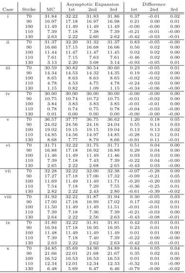
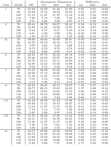
Finally, the results of numerical experiments are shown. Table 3 and Table 4 show the effectiveness of our formula: In particular, the third order expansion generally improves the lower order expansions and provides sufficient accuracies in practice for all cases.
Table 3: Result: λ-SABR Model Asymptotic Expansion Difference Case Strike MC 1st 2nd 3rd 1st 2nd 3rd i 70 31.84 32.22 31.83 31.86 0.37 -0.01 0.02 90 16.97 17.18 16.97 16.98 0.21 0.00 0.01 100 11.49 11.49 11.49 11.49 -0.00 -0.00 0.00 110 7.39 7.18 7.38 7.39 -0.21 -0.01 -0.00 130 2.63 2.22 2.60 2.62 -0.42 -0.03 -0.01 ii 70 31.37 32.20 31.32 31.37 0.83 -0.05 -0.00 90 16.66 17.15 16.68 16.66 0.50 0.02 0.00 100 11.44 11.47 11.47 11.45 0.02 0.02 0.00 110 7.61 7.15 7.63 7.61 -0.46 0.02 0.00 130 3.13 2.20 3.08 3.14 -0.93 -0.05 0.01 iii 70 30.59 30.82 30.54 30.60 0.23 -0.05 0.01 90 14.34 14.53 14.32 14.35 0.19 -0.02 0.00 100 8.65 8.63 8.63 8.65 -0.02 -0.02 0.00 110 4.78 4.53 4.75 4.78 -0.24 -0.03 0.00 130 1.15 0.82 1.09 1.15 -0.34 -0.06 -0.00 iv 70 30.00 30.00 30.00 30.00 -0.00 -0.00 0.00 90 10.75 10.74 10.72 10.75 -0.01 -0.02 0.00 100 3.84 3.83 3.83 3.85 -0.01 -0.01 0.00 110 0.78 0.74 0.75 0.78 -0.04 -0.03 -0.00 130 0.01 0.00 0.00 0.00 -0.00 -0.00 -0.00 v 70 36.57 37.77 36.75 36.62 1.20 0.18 0.05 90 24.02 24.56 24.16 24.04 0.55 0.14 0.03 100 19.02 19.15 19.15 19.04 0.13 0.13 0.02 110 14.85 14.56 14.97 14.85 -0.28 0.12 0.01 130 8.68 7.77 8.79 8.66 -0.91 0.11 -0.01 vi 70 31.71 32.22 31.75 31.71 0.51 0.04 0.00 90 16.88 17.18 16.92 16.89 0.29 0.04 0.00 100 11.46 11.49 11.49 11.46 0.03 0.03 0.00 110 7.39 7.18 7.43 7.39 -0.22 0.04 -0.00 130 2.65 2.22 2.68 2.65 -0.43 0.03 -0.00 vii 70 32.28 32.22 32.00 32.38 -0.07 -0.28 0.09 90 17.27 17.18 17.06 17.32 -0.09 -0.21 0.05 100 11.69 11.49 11.49 11.71 -0.20 -0.20 0.03 110 7.54 7.18 7.29 7.55 -0.36 -0.25 0.01 130 2.82 2.22 2.43 2.80 -0.61 -0.39 -0.02 viii 70 31.92 32.22 31.87 31.94 0.30 -0.05 0.03 90 17.00 17.18 16.99 17.02 0.17 -0.02 0.01 100 11.50 11.49 11.49 11.51 -0.01 -0.01 0.01 110 7.39 7.18 7.36 7.39 -0.21 -0.03 0.00 130 2.64 2.22 2.56 2.63 -0.43 -0.08 -0.01 ix 70 31.80 32.22 31.81 31.81 0.42 0.01 0.01 90 16.94 17.18 16.95 16.95 0.23 0.01 0.01 100 11.48 11.49 11.49 11.49 0.01 0.01 0.00 110 7.39 7.18 7.40 7.39 -0.22 0.00 -0.00 130 2.63 2.22 2.62 2.63 -0.42 -0.01 -0.01 x 70 34.85 35.69 34.90 34.89 0.84 0.05 0.04 90 21.66 22.01 21.68 21.67 0.35 0.02 0.01 100 16.52 16.53 16.53 16.53 0.01 0.01 0.00 110 12.34 12.01 12.34 12.33 -0.32 0.01 -0.00 130 6.48 5.69 6.47 6.46 -0.79 -0.00 -0.02 4.2 Calibration
This subsection applies SABR,λ-SABR and Heston models to calibration of the market prices of the WTI futures American option on July 1, 2009. American options on WTI futures are plain-vanilla options in NYMEX that is a part of CME Group.
In particular, our goal in the next subsection is to evaluate average options with two-month maturity(AUG09), four-month maturity(OCT09) and sixteen-month
ma-Table 4: Result: Heston Model Asymptotic Expansion Difference Case Strike MC 1st 2nd 3rd 1st 2nd 3rd i 70 31.39 32.20 31.40 31.35 0.81 0.01 -0.04 90 16.45 17.15 16.72 16.43 0.70 0.27 -0.02 100 11.14 11.47 11.47 11.14 0.32 0.32 -0.01 110 7.28 7.15 7.58 7.29 -0.13 0.30 0.01 130 2.91 2.20 3.00 2.95 -0.71 0.09 0.04 ii 70 30.41 30.79 30.27 30.41 0.38 -0.14 0.01 90 13.99 14.48 14.06 13.97 0.49 0.07 -0.02 100 8.44 8.57 8.57 8.43 0.13 0.13 -0.00 110 4.81 4.48 4.90 4.81 -0.33 0.09 0.00 130 1.45 0.79 1.32 1.47 -0.66 -0.13 0.02 iii 70 30.00 30.00 30.00 30.01 -0.00 -0.00 0.01 90 10.70 10.73 10.72 10.71 0.04 0.02 0.01 100 3.70 3.82 3.82 3.68 0.12 0.12 -0.01 110 0.75 0.73 0.75 0.74 -0.02 -0.00 -0.01 130 0.02 0.00 0.00 0.01 -0.02 -0.01 -0.01 iv 70 35.25 37.74 35.54 35.18 2.49 0.29 -0.07 90 23.26 24.52 23.65 23.23 1.27 0.39 -0.02 100 18.70 19.11 19.11 18.69 0.41 0.41 -0.00 110 14.96 14.52 15.40 14.98 -0.44 0.43 0.01 130 9.52 7.74 9.94 9.58 -1.78 0.42 0.06 v 70 31.27 32.20 31.26 31.25 0.93 -0.01 -0.02 90 16.56 17.15 16.65 16.56 0.59 0.08 -0.00 100 11.38 11.47 11.47 11.38 0.08 0.08 -0.00 110 7.57 7.15 7.66 7.58 -0.42 0.09 0.00 130 3.11 2.20 3.14 3.13 -0.91 0.03 0.02 vi 70 32.83 34.25 33.10 32.67 1.42 0.27 -0.16 90 18.77 20.15 19.63 18.63 1.37 0.86 -0.14 100 13.62 14.61 14.61 13.52 0.98 0.98 -0.10 110 9.73 10.15 10.66 9.67 0.42 0.93 -0.07 130 4.94 4.25 5.40 4.98 -0.68 0.47 0.04 vii 70 31.42 32.20 31.43 31.38 0.78 0.01 -0.05 90 16.40 17.15 16.74 16.37 0.75 0.34 -0.03 100 11.05 11.47 11.47 11.05 0.41 0.41 -0.01 110 7.19 7.15 7.57 7.20 -0.03 0.38 0.01 130 2.87 2.20 2.97 2.91 -0.67 0.10 0.04 viii 70 31.35 32.20 31.36 31.32 0.85 0.01 -0.03 90 16.51 17.15 16.70 16.50 0.65 0.19 -0.01 100 11.25 11.47 11.47 11.25 0.22 0.22 -0.00 110 7.40 7.15 7.61 7.41 -0.25 0.21 0.01 130 2.98 2.20 3.05 3.01 -0.78 0.07 0.03 ix 70 33.77 35.66 34.04 33.66 1.88 0.27 -0.12 90 20.75 21.98 21.30 20.68 1.23 0.55 -0.06 100 15.89 16.50 16.50 15.86 0.60 0.60 -0.04 110 12.05 11.98 12.66 12.04 -0.08 0.61 -0.01 130 6.83 5.66 7.27 6.89 -1.17 0.45 0.06
turity(OCT10) on July 1, 2009. Note that the underlying price of an average option is the average of the settlement prices of the first nearby WTI futures contract during the last one month prior to the maturity of the average option. Also, the expiration of an average option is the last business day of a calendar month, while trading of a WTI futures contract usually ceases on the third business day prior to the twenty-fifth calendar day. Hence, the WTI futures and their American options with two consecutive maturities are relevant for pricing an average options with calibration to plain-vanilla option prices.
In this analysis, the underlying asset prices are the average prices during August 2009 for the two-month maturity(AUG09), October 2009 for the four-month matu-rity(OCT09) and during October 2010 for the sixteen-month maturity(OCT10) of rel-evant futures; the relrel-evant futures are SEP09 and OCT09 for the two-month maturity, NOV09 and DEC09 for the four-month maturity, and NOV10 and DEC10 for the
sixteen-month maturity. 5 Prices of SEP09, OCT09, NOV09, DEC09, NOV10 and DEC10 on July 1, 2009 are 70.27, 71.08, 71.78, 72.36, 76.06 and 76.4, respectively.
American options with two and three-month maturities are traded almost everyday while options with longer maturities are traded occasionally except options on DEC futures. For example, the volumes of trades of American futures options on July 1, 2009 are listed in Table 5.
Table 5: Volumes of Trades on July 1 2009(1000 barrel)
Strike SEP09 OCT09 NOV09 DEC09 NOV10 DEC10
50 (Put) 4,220 0 0 370 0 4 55 (Put) 262 410 0 2,250 0 400 60 (Put) 2,302 2,800 5 6,605 0 0 65 (Put) 2,270 1,200 40 900 0 100 70 (Put) 501 156 1 3,575 0 0 75 (Call) 350 105 100 5 0 0 80 (Call) 1,237 116 245 901 0 0 85 (Call) 1,300 0 0 1,001 0 0 90 (Call) 70 1,200 0 415 0 250 95 (Call) 0 0 0 1 0 0 100 (Call) 100 0 0 2,686 0 1,414
For pricing OTC average options, if there are no trades of the relevant American options, practitioners refer to the implied volatilities of the settlement prices of the American options. The settlement prices are announced every day for the contracts with positive open interests. Those settlement prices rarely show unreasonable move-ments, which indicates that those prices can be used for the targets of the calibration. For computational efficiency, the settlement prices of American options are trans-formed to those of the European options before calibration: More precisely, after an implied volatility of each American option price is estimated under a binomial version of the Black-Scholes model, the corresponding European option price is computed. Here-after, this European option price is called the“transformed CME” option price. Then, calibration is implemented against the“transformed CME” option prices with differ-ent strikes simultaneously, where out-of-the-money (OTM) and at-the money (ATM) prices are used for the calibration; the strikes of the options range usd 50 to usd 100 with every five dollars. 6
Moreover, the stochastic volatility models used for calibration to the “transformed CME” option prices are the following:
(i) SABR model (β1=β2 = 0.5 in (7) and (8) withλ1=λ2 = 0 in (9) and (10)) (ii) SABR model (β1=β2 = 1 in (7) and (8) withλ1 =λ2 = 0 in (9) and (10))
5
Trading of SEP09(OCT09) ceases before the end of August(September) 2009. Also, trading of NOV09(DEC09) ceases before the end of October(November) 2009 and trading of NOV10(DEC10) ceases before the end of October(November) 2010.
(iii) λ-SABR model (β1=β2 = 0.5 in (7) and (8)) (iv) λ-SABR model (β1=β2 = 1 in (7) and (8))
(v) Heston model
Note that the drifts of the underlying asset processes are set to be zero (α1(t) =α2(t) = 0) due to the futures contracts. Also,v1andv2are fixed to be one (v1=v2= 1) because the initial values of volatilities can be adjusted. Then, plain-vanilla European option prices are computed by the formula of Hagan et.al.[7] for SABR model, our third order asymptotic expansion formula for λ-SABR model and the formula of [8] for Heston model.
The calibrated parameters are obtained through minimization of the sum of the squared differences between model-based and transformed CME call option prices. That is,
min Θ
∑
K
(Model Based Option Price(T, K)−Transformed CME Option Price(T, K))2,
whereT andK denote maturities (SEP09, OCT09, NOV09, DEC09, Nov10 or DEC10) and strike prices (usd 50 to usd 100 with every five dollars), respectively. Also, Θ stands for the set of parameters for calibration. Note that our price-based calibration above is similar to the implied volatility-based calibration weighted by Vega for adjustment of illiquidity in West[21] 7, because the values of options with closer to ATM are more sensitive to the volatility change.
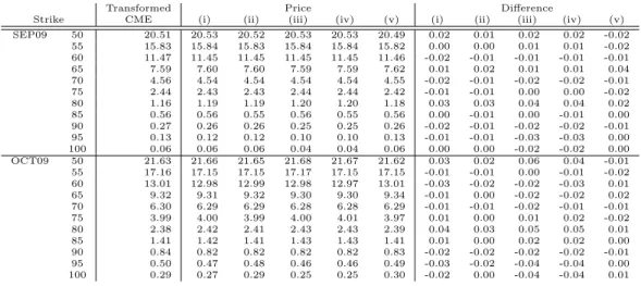
Parameters from calibration are reported in Table 6, 7 and 8. The calibrated and transformed call option prices are shown in Table 9, 10 and 11: “-” in columns of Price and Difference in the tables means that the settlement prices are not announced.
Table 6: Parameters(SEP09, OCT09)
σ(0) V(0) λ θ ν ρ SEP09 (i) 3.607 - - - 1.427 -0.225 (ii) 0.433 - - - 1.519 -0.369 (iii) 3.606 - 0.008 1.788 1.434 -0.209 (iv) 0.434 - 0.093 0.140 1.522 -0.342 (v) - 0.209 0.334 0.607 1.478 -0.377 OCT09 (i) 3.623 - - - 1.140 -0.188 (ii) 0.433 - - - 1.252 -0.363 (iii) 3.616 - 0.016 1.792 1.175 -0.170 (iv) 0.435 - 0.087 0.140 1.227 -0.335 (v) - 0.207 0.226 0.804 1.256 -0.372
It is observed that while all models generally provide good calibration at first glance, the Feller condition(2λθ ≥ ν2) necessary for the positive variance process in Heston model (v) is not satisfied for all contracts. In other words, the smiles of implied
Table 7: Parameters(NOV09, DEC09) σ(0) V(0) λ θ ν ρ NOV09 (i) 3.606 - - - 1.000 -0.190 (ii) 0.430 - - - 1.109 -0.383 (iii) 3.614 - 0.035 1.838 0.993 -0.172 (iv) 0.430 - 0.016 0.163 1.086 -0.357 (v) - 0.211 0.084 0.887 1.058 -0.392 DEC90 (i) 3.519 - - - 0.993 -0.172 (ii) 0.419 - - - 1.098 -0.365 (iii) 3.523 - 0.007 1.590 0.977 -0.152 (iv) 0.419 - 0.008 0.223 1.063 -0.340 (v) - 0.217 0.024 0.515 1.019 -0.378
Table 8: Parameters(NOV10, DEC10)
σ(0) V(0) λ θ ν ρ NOV10 (i) 2.771 - - - 0.511 -0.126 (ii) 0.323 - - - 0.630 -0.384 (iii) 2.773 - 0.001 2.765 0.494 -0.112 (iv) 0.322 - 0.005 0.326 0.610 -0.363 (v) - 0.016 0.367 0.618 0.834 -0.404 DEC10 (i) 2.742 - - - 0.581 -0.112 (ii) 0.321 - - - 0.653 -0.371 (iii) 2.750 - 0.000 2.753 0.555 -0.098 (iv) 0.321 - 0.002 0.331 0.626 -0.350 (v) - 0.011 0.365 0.617 0.865 -0.390
Table 9: Calibration to Futures Call Option Prices(SEP09, OCT09)(usd)
Transformed Price Difference
Strike CME (i) (ii) (iii) (iv) (v) (i) (ii) (iii) (iv) (v) SEP09 50 20.51 20.53 20.52 20.53 20.53 20.49 0.02 0.01 0.02 0.02 -0.02 55 15.83 15.84 15.83 15.84 15.84 15.82 0.00 0.00 0.01 0.01 -0.02 60 11.47 11.45 11.45 11.45 11.45 11.46 -0.02 -0.01 -0.01 -0.01 -0.01 65 7.59 7.60 7.60 7.59 7.59 7.62 0.01 0.02 0.01 0.01 0.04 70 4.56 4.54 4.54 4.54 4.54 4.55 -0.02 -0.01 -0.02 -0.02 -0.01 75 2.44 2.43 2.43 2.44 2.44 2.42 -0.01 -0.01 0.00 0.00 -0.02 80 1.16 1.19 1.19 1.20 1.20 1.18 0.03 0.03 0.04 0.04 0.02 85 0.56 0.56 0.55 0.56 0.55 0.56 0.00 -0.01 0.00 -0.01 0.00 90 0.27 0.26 0.26 0.25 0.25 0.26 -0.02 -0.01 -0.02 -0.02 -0.01 95 0.13 0.12 0.12 0.10 0.10 0.13 -0.01 -0.01 -0.03 -0.03 0.00 100 0.06 0.06 0.06 0.04 0.04 0.06 0.00 0.00 -0.02 -0.02 0.00 OCT09 50 21.63 21.66 21.65 21.68 21.67 21.62 0.03 0.02 0.06 0.04 -0.01 55 17.16 17.15 17.15 17.17 17.15 17.15 -0.01 -0.01 0.00 -0.01 -0.02 60 13.01 12.98 12.99 12.98 12.97 13.01 -0.03 -0.02 -0.02 -0.03 0.01 65 9.32 9.31 9.32 9.30 9.30 9.34 -0.01 0.00 -0.02 -0.02 0.02 70 6.30 6.29 6.29 6.28 6.28 6.29 -0.01 -0.01 -0.02 -0.01 -0.01 75 3.99 4.00 3.99 4.00 4.01 3.97 0.01 0.00 0.01 0.02 -0.02 80 2.38 2.42 2.41 2.43 2.43 2.39 0.04 0.03 0.05 0.05 0.01 85 1.41 1.42 1.41 1.43 1.43 1.41 0.01 0.00 0.02 0.02 0.00 90 0.84 0.82 0.82 0.82 0.82 0.83 -0.02 -0.02 -0.02 -0.02 -0.01 95 0.50 0.47 0.48 0.46 0.46 0.49 -0.03 -0.02 -0.04 -0.04 0.00 100 0.29 0.27 0.29 0.25 0.25 0.30 -0.02 0.00 -0.04 -0.04 0.01
volatilities in American options on WTI futures are so extreme that Heston model has difficulty in calibration under the Feller condition.
Table 10: Calibration to Futures Call Option Prices(NOV09, DEC09)(usd)
Transformed Price Difference
Strike CME (i) (ii) (iii) (iv) (v) (i) (ii) (iii) (iv) (v) NOV09 50 22.59 22.65 22.63 22.66 22.66 22.59 0.06 0.04 0.07 0.07 0.01 55 18.26 18.26 18.26 18.26 18.26 18.25 0.01 0.00 0.01 0.01 -0.01 60 14.24 14.21 14.22 14.20 14.20 14.24 -0.03 -0.02 -0.04 -0.04 0.00 65 10.65 10.62 10.63 10.61 10.61 10.66 -0.03 -0.02 -0.04 -0.04 0.01 70 7.61 7.60 7.60 7.60 7.60 7.62 -0.02 -0.01 -0.02 -0.02 0.00 75 5.20 5.21 5.21 5.22 5.22 5.19 0.01 0.01 0.02 0.02 -0.01 80 3.41 3.44 3.43 3.45 3.45 3.41 0.04 0.03 0.05 0.05 0.00 85 2.19 2.22 2.21 2.23 2.22 2.20 0.03 0.02 0.04 0.04 0.01 90 1.42 1.40 1.40 1.41 1.41 1.41 -0.01 -0.02 -0.01 -0.01 -0.01 95 0.91 0.89 0.89 0.88 0.88 0.91 -0.03 -0.02 -0.04 -0.03 -0.01 100 0.58 0.56 0.58 0.54 0.54 0.59 -0.02 0.00 -0.04 -0.04 0.01 DEC09 50 23.49 23.58 23.56 23.59 23.59 23.51 0.09 0.07 0.10 0.10 0.02 55 19.28 19.29 19.29 19.29 19.29 19.28 0.01 0.01 0.01 0.01 0.00 60 15.38 15.32 15.33 15.31 15.31 15.36 -0.06 -0.05 -0.07 -0.07 -0.02 65 11.83 11.78 11.79 11.77 11.77 11.83 -0.05 -0.04 -0.07 -0.06 0.00 70 8.78 8.75 8.76 8.75 8.75 8.78 -0.02 -0.01 -0.02 -0.02 0.00 75 6.28 6.30 6.30 6.31 6.31 6.28 0.02 0.02 0.03 0.03 0.00 80 4.38 4.42 4.41 4.44 4.44 4.38 0.05 0.04 0.06 0.06 0.01 85 3.00 3.05 3.04 3.06 3.06 3.02 0.05 0.04 0.07 0.07 0.03 90 2.11 2.09 2.09 2.10 2.10 2.09 -0.02 -0.02 -0.01 -0.01 -0.02 95 1.47 1.43 1.44 1.43 1.43 1.46 -0.04 -0.03 -0.05 -0.04 -0.01 100 1.02 0.99 1.01 0.96 0.97 1.03 -0.03 -0.01 -0.06 -0.05 0.01
Table 11: Calibration to Futures Call Option Prices(NOV10, DEC10)(usd)
Transformed Price Difference
Strike CME (i) (ii) (iii) (iv) (v) (i) (ii) (iii) (iv) (v) NOV10 50 27.98 28.00 28.02 28.01 28.06 28.05 0.02 0.04 0.03 0.08 0.07 55 - - - -60 20.47 20.39 20.42 20.37 20.39 20.48 -0.08 -0.05 -0.10 -0.08 0.01 65 - - - -70 14.08 14.05 14.06 14.04 14.03 14.09 -0.03 -0.02 -0.04 -0.05 0.01 75 11.45 11.44 11.43 11.44 11.42 11.44 -0.01 -0.02 -0.01 -0.03 -0.01 80 9.24 9.21 9.19 9.21 9.19 9.17 -0.03 -0.05 -0.03 -0.04 -0.07 85 7.35 7.35 7.32 7.35 7.34 7.29 0.00 -0.03 0.00 -0.01 -0.06 90 5.74 5.82 5.80 5.83 5.83 5.78 0.09 0.06 0.09 0.09 0.04 95 - - - -100 3.56 3.62 3.64 3.61 3.64 3.65 0.06 0.08 0.05 0.08 0.08 DEC10 50 28.46 28.59 28.55 28.60 28.60 28.53 0.13 0.09 0.14 0.14 0.07 55 24.64 24.65 24.64 24.64 24.64 24.65 0.01 0.01 0.00 0.00 0.01 60 21.07 20.98 20.99 20.96 20.96 21.01 -0.09 -0.08 -0.11 -0.11 -0.06 65 17.73 17.62 17.64 17.60 17.61 17.67 -0.12 -0.09 -0.13 -0.13 -0.07 70 14.61 14.61 14.63 14.60 14.61 14.65 -0.01 0.01 -0.01 -0.01 0.04 75 11.91 11.97 11.98 11.98 11.98 12.00 0.06 0.07 0.07 0.07 0.09 80 9.68 9.72 9.71 9.74 9.74 9.72 0.04 0.03 0.05 0.05 0.04 85 7.81 7.84 7.82 7.86 7.85 7.82 0.03 0.01 0.05 0.04 0.01 90 6.29 6.30 6.27 6.31 6.31 6.27 0.01 -0.03 0.02 0.01 -0.02 95 5.04 5.06 5.03 5.06 5.06 5.04 0.02 -0.02 0.02 0.02 0.00 100 4.15 4.07 4.05 4.06 4.06 4.07 -0.07 -0.10 -0.09 -0.09 -0.08
When the Feller condition is not satisfied, the volatility process of Heston model is not well-defined. Thus, Heston model is not adopted for pricing average options in the next subsection, where the estimated average prices based the calibration are compared with CME Group’s settlement prices.
Also, note thatλ≈0 in the calibrated λ-SABR for all of maturities and hence the model is not distinguished with SABR model. We also remark that the estimates of parameters(λ,θ) inλ-SABR and Heston models are sometimes are not stable because the estimates often converge to local optima.
4.3 Average Option Prices with Calibrated Parameters
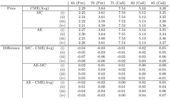
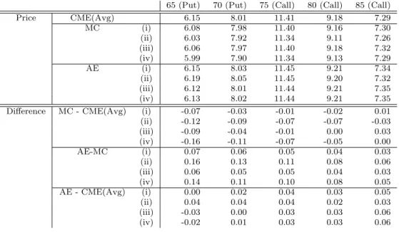
This subsection shows the approximate prices of average options with calibrated pa-rameters and compares the prices with the ones obtained by Monte Carlo simulations as well as with the settlement prices in CME Group.
Note that there are few trades of average options in CME Group since average options are traded mainly in OTC market; for instance, there were no trades for AUG09 , OCT09 and OCT10 on July 1, 2009 except only 125 barrel trades for 70 Put of AUG09. However, there are no official prices in the OTC market. On the other hand, the settlement prices in CME Group are announced every day for the contracts with positive open interests. Thus, we use the settlement prices of average options as the reference prices.
In Monte Caro simulation, the term is divided into 195 time-steps for AUG09, 305 time-steps for OCT09 and 600 time-steps for OCT10, and the number of trials are set to be 10,000,000. 8
The interest rates used for discounting are 0.41% for AUG09, 0.77% for OCT09 and 1.62% for OCT10. The correlation between two underlying futures prices, SEP09 and OCT09 is calculated based on the daily rates of returns from April 30, 2009 to July 1, 2009; the correlation is estimated as 0.99920. The correlation between NOV09 and DEC09 is calculated based on the daily rates of returns from February 27, 2009 to July 1, 2009; it is estimated as 0.99941. The correlation between NOV10 and DEC10 is calculated based on the daily rates of returns from February 29, 2008 to July 1, 2009; it is estimated as 0.99990. The average option prices computed under those conditions are reported in Table 12, 13 and 14.
Compared with prices computed by Monte Carlo simulations, the approximations with β = 1((ii),(iv)) are less accurate than those with β = 0.5((i),(iii)). Because the asymptotic expansion method is based on an expansion around a normal distribution and the distribution of the underlying asset price is closer to a normal whenβ is closer to zero, the smaller is β, the approximation becomes more accurate in general.
It is also observed in “MC - CME(Avg)” that the settlement prices of AUG09, OCT09 and OCT10 in CME Group are generally close to the average options prices with calibrated parameters, which implies that the settlement prices of average options may be given consistently with the prices of WTI futures American options.
As previously noted, λ ≈ 0 is estimated in calibration under λ-SABR model and the estimates of parameters(λ,θ) are sometimes are unstable. Hence, at least for above examined cases, SABR model with β = 0.5 seems the better model for calibration to the market prices of the American option on WTI futures as well as for approximation of average options prices.
8In the (λ-)SABR model, when the volatility process becomes non-positive due to discretization, we
setσ(ti+1) =σ(ti) +λθ∆t,S(ti+1) =S(ti) +αS(ti)∆t.Also when the underlying asset price becomes