Parallel algorithms for finding connected components using linear algebra

Lawrence Berkeley National Laboratory

Recent Work

Title

Parallel algorithms for finding connected components using linear algebra

Permalink

https://escholarship.org/uc/item/8ms106vm

Authors

Zhang, Y

Azad, A

Buluç, A

Publication Date

2020-10-01

DOI

10.1016/j.jpdc.2020.04.009

Peer reviewed

eScholarship.org

Powered by the California Digital Library

Parallel Algorithms for Finding Connected Components using Linear Algebra

a_{Department of Informatics, The Graduate University for Advanced Studies, SOKENDAI, Japan} b_{Department of Intelligent Systems Engineering, Indiana University, Bloomington, IN, USA} c_{Computational Research Division, Lawrence Berkeley National Laboratory, Berkeley, CA, USA}

Abstract

Finding connected components is one of the most widely used operations on a graph. Optimal serial algorithms for the problem have been known for half a century, and many competing parallel algorithms have been proposed over the last several decades under various different models of parallel computation. This paper presents a class of parallel connected-component algorithms designed using linear-algebraic primitives. These algorithms are based on a PRAM algorithm by Shiloach and Vishkin and can be designed using standard GraphBLAS operations. We demonstrate two algorithms of this class, one named LACC for Linear Algebraic Connected Components, and the other named FastSV which can be regarded as LACC’s simplification. With the support of the highly-scalable Combinatorial BLAS library, LACC and FastSV outperform the previous state-of-the-art algorithm by a factor of up to 12x for small to medium scale graphs. For large graphs with more than 50B edges, LACC and FastSV scale to 4K nodes (262K cores) of a Cray XC40 supercomputer and outperform previous algorithms by a significant margin. This remarkable performance is accomplished by (1) exploiting sparsity that was not present in the original PRAM algorithm formulation, (2) using high-performance primitives of Combinatorial BLAS, and (3) identifying hot spots and optimizing them away by exploiting algorithmic insights.

1. Introduction

Given an undirected graphG=(V,E) on the set of vertices Vand the set of edgesE, a connected component (CC) is a sub-graph in which every vertex is connected to all other vertices in the subgraph by paths and no vertex in the subgraph is con-nected to any other vertex outside of the subgraph. Finding all connected components in a graph is a well studied problem in graph theory with applications in bioinformatics [1] and scien-tific computing [2,3].

Parallel algorithms for finding connected components also have a long history, with several ingenious techniques applied to the problem. One of the most well-known parallel algorithms is due to Shiloach and Vishkin [4], where they introduced the hooking procedure. The algorithm also uses pointer jumping, a fundamental technique in PRAM (parallel random-access ma-chine) algorithms, for shortcutting. Awerbuch and Shiloach [5] later simplified and improved on this algorithm. Despite the fact that PRAM model is a poor fit for analyzing distributed memory algorithms, we will show in this paper that the Shiloach-Vishkin (SV) and Awerbuch-Shiloach (AS) algorithms admit a very effi-cient parallelization using proper computational primitives and sparse data structures.

Decomposing the graph into its connected components is often the first step in large-scale graph analytics where the goal is to create manageable independent subproblems. Therefore, it is important that connected component finding algorithms can

Email addresses:[email protected](Yongzhe Zhang),[email protected] (Ariful Azad),[email protected](Aydın Buluc¸)

run on distributed memory, even if the subsequent steps of the analysis need not. Several applications of distributed-memory connected component labeling have recently emerged in the field of genomics. The metagenome assembly algorithms repre-sent their partially assembled data as a graph [6,7]. Each com-ponent of this graph can be processed independently. Given that the scale of the metagenomic data that needs to be assembled is already on the order of several TBs, and is on track to grow exponentially, distributed connected component algorithms are of growing importance.

Another application comes from large scale biological net-work clustering. The popular Markov clustering algorithm (MCL) [1] iteratively performs a series of sparse matrix ma-nipulations to identify the clustering structure in a network. Af-ter the iAf-terations converge, the clusAf-ters are extracted by find-ing the connected components on the symmetrized version of the final converged matrix, i.e., in an undirected graph repre-sented by the converged matrix. We have recently developed the distributed-memory parallel MCL (HipMCL) [8] algorithm that can cluster protein similarity networks with hundreds of billions of edges using thousands of nodes on modern super-computers. Since computing connected components is an im-portant step in HipMCL, a parallel connected component algo-rithm that can scale to thousands of nodes is imperative.

In this paper, we present two parallel algorithms based on the SV and AS algorithms. These algorithms are specially de-signed by mapping different operations to the GraphBLAS [9] primitives, which are standardized linear-algebraic functions that can be used to implement graph algorithms. The linear-algebraic algorithm which is derived from the AS algorithm

is named as LACC for linear algebraic connected compo-nents. The second algorithm is a simplification of the SV al-gorithm and is named as FastSV due to its improved conver-gence in practice. FastSV can also be considered a simplifica-tion of LACC. While the initial reasons behind choosing the SV and AS algorithms were simplicity, performance guarantees, and expressibility using linear algebraic primitives, we found that they are never slower than the state-of-the-art distributed-memory algorithm ParConnect [10], and they often outperform ParConnect by several folds.

LACC and FastSV algorithms are published as conference papers [11,12]. This journal paper extends those algorithms by providing a unified framework for CC algorithms in lin-ear algebra. Designing CC algorithms using a standard set of linear-algebraic operations gives a crucial benefit. After an algorithm is mapped to GraphBLAS primitives, we can rely on any library providing high-performance implementations of those primitives. In this paper we use the Combinatorial BLAS (CombBLAS) library [13], a well-known framework for im-plementing graph algorithms in the language of linear alge-bra. Different from the original SV and AS algorithms, our implementations fully exploit vector sparsity and avoids pro-cessing on inactive vertices. We perform several additional op-timizations to eliminate performance hot spots and provide a detailed breakdown of our parallel performance, both in terms of theoretical communication complexity and in experimental results. These algorithmic insights and optimizations result in a distributed algorithm that scales to 4K nodes (262K cores) of a Cray XC40 supercomputer and outperforms previous algo-rithms by a significant margin. We also implemented our al-gorithm using SuiteSparse:GraphBLAS [14], a multi-threaded implementation of the GraphBLAS standard. The performance of the shared-memory implementations is comparable to state-of-the-art CC algorithms designed for share-memory platforms. Distributed-memory LACC and FastSV codes are publicly available as part of the CombBLAS library1_{. Shared-memory}

GraphBLAS implementations are also committed to the LA-Graph Library [15]2_{. This paper is an extension of a conference}

paper [11] published in IPDPS 2019.

2. Background 2.1. Notations

This paper only considers an undirected and unweighted graphG=(V,E) withnvertices andmedges. Given a vertex v, N(v) is the set of vertices adjacent tov. A tree is an undi-rected graph where any two vertices are connected by exactly one path. A directed rooted tree is a tree in which a vertex is designated as the root and all vertices are oriented toward the root. The levell(v) of a vertexvin a tree is 1 plus the number of edges betweenvand the root. The level of the root is 1. A tree is called astarif every vertex is a child of the root (the root

1_{https://bitbucket.org/berkeleylab/combinatorial-blas-2.0/} 2_{https://github.com/GraphBLAS/LAGraph}

is a child of itself). A vertex is called astar vertexis it belongs to a star.

2.2. GraphBLAS

The duality between sparse matrices and graphs has a long and fruitful history [16, 17]. Several independent systems have emerged that use matrix algebra to perform graph oper-ations [13,18,19]. Recently, the GraphBLAS forum defined a standard set of linear-algebraic operations for implementing graph algorithms, leading to the GraphBLAS C API [20]. In this paper, we will use the functions from the GraphBLAS API to describe our algorithms. That being said, our algorithms run on distributed memory while currently no distributed-memory library faithfully implements the GraphBLAS API. The most recent version of the API (1.2.0) is actually silent on distributed-memory parallelism and data distribution. Consequently, while our descriptions follow the API, our implementation will be based on CombBLAS functions [13], which are either seman-tically equivalent in functionality to their GraphBLAS counter-parts or can be composed to match GraphBLAS functionality. 2.3. Related work

Finding connected components of an undirected graph is one of the most well-studied problems in the PRAM (parallel random-access memory) model. A significant portion of these algorithms assume the CRCW (read concurrent-write model). The Awerbuch-Shiloach (AS) algorithm is a sim-plification of the Shiloach-Vishkin (SV) algorithm [4]. The fun-damental data structure in both AS and SV algorithms is a for-est of rooted trees. While AS only keeps the information of the current forest, SV additionally keeps track of the forest in the previous iteration of the algorithm as well as the last time each parent received a new child. The convergence criterion for AS is to check whether each tree is a star whereas SV needs to see whether the last iteration provided any updates to the forest.

Randomization is also a fundamental technique applied to the connected components problem. The random-mate (RM) algorithm, due to Reif [21], flips an unbiased coin for each ver-tex to determine whether it is a parent or a child. Each child then finds a parent among its neighbors. The stars are con-tracted to supervertices in the next iteration as in AS and SV algorithms. All three algorithms described so far (RM, AS, and SV) are work inefficient in the sense that their processor-time product is asymptotically higher than the runtime complexity of the best serial algorithm.

A similar randomization technique allowed Gazit to dis-cover a work-efficient CRCW PRAM algorithm for the con-nected components problem [22]. His algorithm runs with O(m) optimal work andO(log(n)) span. More algorithms fol-lowed achieving the same work-span bound but improving the state-of-the-art by working with more restrictive models such as EREW (exclusive-read exclusive-write) [23], solving more general problems such as minimum spanning forest [24] whose output can be used to infer connectivity, and providing first im-plementations [25].

The literature on distributed-memory connected compo-nent algorithms and their complexity analyses, is significantly

Algorithm 1 The skeleton of the AS algorithm. Inputs: an undirected graphG(V,E).Output:The parent vector f

1: procedureAwerbuch-Shiloach(G(V,E)) 2: forevery vertexvinVdo.Initialize 3: f[v]←v

4: repeat

5: .Step1: Conditional star hooking 6: forevery edge{u,v}inEdo in parallel 7: ifubelongs to a star andf[u]>f[v]then 8: f[f[u]]← f[v]

9: .Step2: Unconditional star hooking 10: forevery edge{u,v}inEdo in parallel 11: ifubelongs to a star andf[u],f[v]then 12: f[f[u]]← f[v]

13: .Step3: Shortcutting

14: forevery vertexvinVdo in parallel

15: gf[v]← f[f[v]]

16: forevery vertexvinVdo in parallel

17: ifvdoes not belongs to a starthen

18: f[v]←gf[v]]

19: untilfremains unchanged 20: returnf

sparser than the case for PRAM algorithms. The state-of-the-art prior to our work is the ParConnect algorithm [10], which is based on both the SV algorithm and parallel breadth-first search (BFS). Slota et al. [26] developed a distributed memory Mul-tistep method that combines parallel BFS and label propaga-tion technique. There have also been implementapropaga-tions of con-nected component algorithms in PGAS (partitioned global ad-dress space) languages [27] in distributed memory. Viral Shah’s PhD thesis [28] presents a data-parallel implementation of the AS algorithm that runs on Matlab*P, a distributed variant of Matlab that is now defunct. Shah’s implementation uses vastly different primitives than our own and solely relies on manipu-lating dense vectors, hence is limited in scalability.

Kiveras et al. [29] proposed the Two-Phase algorithm for MapReduce systems. Such algorithms tend to perform poorly in tightly-couple parallel systems our work targets compared to the loosely-coupled architectures that are optimized for cloud workloads. There is also recent work on parallel graph con-nectivity within the theory community, using various different models of computation [30,31]. These last two algorithms are not implemented and its is not clear if such complex algorithms can be competitive in practice on real distributed-memory par-allel systems.

3. Variants of the Shiloach-Vishkin (SV) algorithm

At first, we discuss the general framework of the SV algo-rithms. Based on this framework, we discuss two algorithmic variants that will be designed using linear algebra.

The SV algorithm and its variants maintain a forest (a col-lection of directed rooted trees), where each tree represents a connected component at the current stage of the algorithm. To represent trees, the algorithm maintains a parent vector f,

Algorithm 2Finding vertices in stars.Inputs:a graphG(V,E) and the parent vectorf.Output:Thestarvector.

1: procedureStarcheck(G(V,E),f)

2: forevery vertexvinVdo in parallel .Initialize 3: star[v]←true

4: gf[v]←f[f[v]]

5: .Exclude every vertexvwithl(v)>2 and its grandparent 6: forevery vertexvinVdo in parallel

7: if f[v],gf[v]then 8: star[v]←false

9: star[gf[v]]←false

10: .In nonstar trees, exclude vertices at level 2 11: forevery vertexvinVdo in parallel 12: star[v]←star[f[v]]

13: returnstar

where f[v] stores the parent of a vertex v. All vertices in a tree belong to the same component, and at termination of the algorithm, all vertices in a connected component belong to the same tree. Each tree has a designated root (a vertex having a self-loop) that serves as the representative vertex for the corre-sponding component.

The algorithm begins with n single-vertex trees and iter-atively merges trees until no such merging is possible. This merging is performed by a process calledtree hooking, where the root of a tree becomes a child of a vertex in another tree. Between two subsequent iterations, the algorithm reduces the height of trees by a process calledshortcutting, where a vertex becomes a child of its grandparent.

The original Shiloach-Vishkin algorithm and its successor the Awerbuch-Shiloach algorithm used a conditional hooking step as well as an unconditional hooking step in every iteration. Conditional hooking of a rootuis allowed only whenu’s id is larger than the vertex whichu is hooked into. Unconditional hooking can hook any trees that remained unchanged in the preceding conditional hooking. With this general framework, the SV algorithm is guaranteed to finish inO(logn) iterations, where each iteration performsO(m) parallel work.

3.1. The Awerbuch-Shiloach (AS) algorithm

Awerbuch and Shiloach simplified the SV algorithm by al-lowing only stars to be hooked on to other trees [5]. Similar to the SV algorithm, the AS algorithm also needs both conditional and unconditional star hooking and shortcutting operations. To track vertices in stars, the algorithm maintains a Boolean vec-torstar. For every vertexv,star[v] istrueifvis a star vertex, star[v] isfalseotherwise.

Description of the algorithm. Algorithm1 describes the main components of the AS algorithm. Initially, every vertex is its own parent, creating n single-vertex stars (lines 2-3 of Algorithm1). In every iteration, the algorithm performs three operations: (a) conditional hooking, (b) unconditional hooking and (c) shortcutting. In the conditional hooking (lines 6-8), ev-ery edge{u,v}is scanned to see if (a)uis in a star and (b) the parent ofu is greater than the parent ofv. If these conditions are satisfied, f[u] is hooked to f[v] by making f[v] the parent

0 2 5 6 3 1 4 0 2 5 6 3 1 4 0 2 5 6 3 1 4 0 2 5 6 3 1 4 0 2 5 6 3 1 4 0 2 5 6 3 1 4

(a) A connected graph (b) Initially, every vertex is a star (c) Conditional hooking of stars

(e) Unconditional hooking of stars (f) Shortcutting (d) Check for stars

A nonstar A star

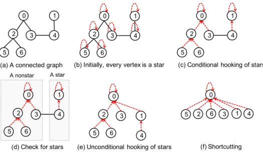
Figure 1: An illustrative example of the AS algorithm. Edges are shown in solid black edges. A dashed arrowhead connects a child with its parent. (a) An undirected and unweighted graph. (b) Initially, every vertex forms a singleton tree. (c) After conditional hooking. Here, we only show edges connecting vertices from different trees. (d) Identifying vertices in stars (see Figure2for details). (e) After unconditional hooking: the star rooted at vertex 1 is hooked onto the left tree rooted at vertex 0. (f) After shortcutting, all vertices belong to stars. The algorithm returns with a connected component.

0 2 5 6 0 2 3 5 6 0 2 3 5 6 3 1 4 Belongs to a a star Does not belong to a star 1

4

1 4

(a) initialize: every

vertex is in a star (b) Mark all vertices except vertices at level 2

(c) Mark vertices at level 2

Figure 2: Finding star vertices. Star and nonstar vertices are shown with unfilled and filled circles, respectively. A dashed arrowhead connects a child with its parent. (a) Initially, every vertex is assumed to be a star vertex. (b) Every vertexvwithl(v)>2 and its grandparent are marked as nonstar vertices. (c) In a nonstar tree, vertices at level 2 are marked as nonstar vertices.

of f[u]. The remaining stars then get a chance to hook uncondi-tionally (lines 10-12). In the shortcutting step, the grandparent of all vertices are identified and stored in the gf vector (lines 14-15). Thegf vector is then used to update parents of all ver-tices (lines 16-18). Figure 1 shows the execution of different steps of the AS algorithm.

Algorithm 2 and Figure 2 describe how star vertices are identified based on the parent vector. Initially, every vertexv is assumed to be a star vertex by settingstar[v] totrue(line 3 of Algorithm2). The algorithm marks vertices as nonstars if any of the following three conditions is satisfied:

• v’s parent and grandparent are not the same vertex. In this case,l(v)>2 as shown in Figure2(b)

• Ifvis a nonstar vertex, then its grandparent is also a non-star vertex (Figure2(b) and and line 9 of Algorithm2)

• Ifv’s parent is a nonstar, thenvis also a nonstar vertex (Figure2(c) and lines 11-12 of Algorithm2)

The AS algorithm terminates when every tree becomes a star and the parent vector f is not updated in the latest

itera-tion. The algorithm terminates inO(logn) iterations. Hence, the algorithm runs inO(logn) time usingm+nprocessors in the PRAM model.

3.2. A simplified SV algorithm with fast convergence

While the AS algorithm is simpler than the original SV al-gorithm, it still needs to identify stars before every hooking op-eration. This star finding step can incur significant performance overhead, especially when the algorithm is run in distributed memory systems. Here, we discuss a variant of the SV algo-rithm that is simpler and faster than the AS algoalgo-rithm in prac-tice.

Notice that if we remove unconditional hooking from SV, the algorithm is still correct, but it no longer guarantees the O(logn) iterations in the worst case. Nevertheless, practi-cal parallel algorithms often remove the unconditional hook-ing [32,33] because it needs to keep track of unchanged trees (also known as stagnant trees), which is expensive, especially in distributed memory. In a recent paper, we developed an algo-rithm called FastSV [12] that has only one hooking phase fol-lowed by shortcutting in every iteration. In the hooking phase,

Algorithm 3The skeleton of the FastSV algorithm. Input: a graphG(V,E).Output:The parent vector f

1: procedureFastSV(G(V,E))

2: forevery vertexu∈Vdo in parallel.Initialize 3: f[u],gf[u]←v

4: repeat

5: .Step 1: Hooking phase

6: forevery edge{u,v}inEdo in parallel 7: ifgf[u]>gf[v]then

8: f[f[u]]←gf[v]

9: f[u]←gf[v]

10: .Step 2: Shortcutting

11: forevery vertexuinVdo in parallel

12: if f[u]>gf[u]then

13: f[u]←gf[u]

14: .Step 3: Calculate grandparent

15: forevery vertexuinVdo in parallel

16: gf[u]← f[f[u]] 17: untilgf remains unchanged 18: returnf

FastSV explores any opportunities to hook a subtree onto an-other tree if a “suitable” edge between them can be found. Hav-ing this simplified constraint, FastSV not only avoids the cycle in the tree updating, but also makes it possible to employ more powerful hooking strategies while retaining the low computa-tion cost. The shortcutting is the same as the AS algorithm, which shortens the distance of each vertex to the root.

Description of the algorithm. Algorithm3describes the complete FastSV algorithm3_{. The initialization is the same as}

the AS algorithm which createsn single-vertex trees, and the grandparent of each vertex is also initialized and stored in the vectorgf. In each iteration, the algorithm performs three oper-ations: (a) stochastic hooking, (b) aggressive hooking and (c) shortcutting. Due to the similarity of the first two operations, they are combined into a single step called the hooking phase (line 6-9). In this phase, we compare the grandparent ofuandv for every edge{u,v}inE. If the conditiongf[u]>gf[v] is sat-isfied, we hook both f[u] anduontogf[v],v’s grandparent in the previous iteration. Here, hooking f[u] togf[v] corresponds to thestochastic hookingand hookingutogf[v] corresponds to theaggressive hooking. Then, in the shortcutting step (line 11-13), every vertexumodifies its pointer togf[u] ifgf[u]> f[u] is satisfied. In the end of each iteration, the grandparents of all vertices are recalculated and stored in thegf vector (lines 15-16), and the algorithm’s termination is based on the stabi-lization of thegf vector instead off, which is also correct and is proved to be a better termination condition in practice [12].

4. The AS and FastSV algorithms using linear algebra In this section, we design the AS and FastSV algorithms using the GraphBLAS API [9]. We used GraphBLAS API to

3_{Algorithm3is presented in a prior work [12]. It is described here for} completeness and readability

describe our algorithms because the API is more expressive, well-thought-of, and future proof. Below we give an informal description of GraphBLAS functions used in our algorithms. Formal descriptions can be found in the API document [34].

The function GrB Vector nvals retrieves the number of stored elements (tuples) in a vector.GrB Vector extractTuples extracts the indices and values associated with nonzero entries of a vector. In all other GraphBLAS functions we use, the first parameter is the output, the second parameter is the mask that determines to which elements of the output should the result of the computation be written into, and the third parameter de-termines the accumulation mode. We will refrain from using an accumulator and instead be performing an assignment in all cases; hence our third parameter is alwaysGrB NULL.

• The functionGrB mxv multiplies a matrix with a vector on a semiring, outputting another vector. The GraphBLAS API does not provide specialized function names for sparse vs. dense vectors and matrices, but instead allows the implemen-tation to internally call different subroutines based on input sparsity. In our use case, matrices are always sparse whereas vectors start out dense and get sparse rapidly. GrB mxv op-erates on a user defined semiring objectGrB Semiring. We refer to a semiring by listing its scalar operations, such as the (multiply, add) semiring. Our algorithm uses the (Select2nd, min) semiring with theGrB mxv function where Select2nd returns its second input and min returns the minimum of its two inputs.

• The vector variant ofGrB extractextracts a sub-vector from a larger vector. The larger vector from which we are extracting elements from is the fourth parameter. The fifth parameter is a pointer to the set of indices to be extracted, which also determines the size of the output vector.

• The vector variant of theGrB assign function that assigns the entries of a GraphBLAS vector (u) to another, potentially larger, vectorw. The vector whose entries we are assigning to is the fourth parameteru. The fifth parameter is a pointer to the set of indices of the outputwto be assigned.

• The vector variant ofGrB eWiseMultperforms element-wise (general) multiplication on the intersection of elements of two vectors. The multiplication operation is provided as a

GrB Semiringobject in the fourth parameter and the input

vectors are passed in the fifth and sixth parameters.

We will refrain from making a general complexity analysis of these operations as the particular instantiations have different complexity bounds. Instead, we will analyze their complexities as they are used in our particular algorithms.

4.1. LACC: The AS algorithm using linear algebra

At first, we design the AS algorithm (Algorithm1and2) us-ing linear algebra. As mentioned in the Introduction, the linear-algebraic design of the AS algorithm is called LACC, follow-ing the namfollow-ing used in the conference paper which this journal

Algorithm 4 Conditional hooking of stars. Inputs: an adja-cency matrixA, the parent vectorf, the star-membership vector star.Output: Updatedf. (NULL is denoted by∅)

1: procedureCondHook(A, f,star)

2: Sel2ndMin←a (select2nd, min) semiring

3: .Step1: fn[i] stores the parent (with the minimum id) of a neighbor of vertexi. Next,fn[i] is replaced by min{fn[i],f[i]} 4: GrB mxv(fn,star,∅, Sel2ndMin,A, f,∅)

5: GrB eWiseMult(fn,∅,∅, GrB MIN T,fn, f,∅);

6: .Step2: Parents of hooks (hooks are nonzero indices infn) 7: GrB eWiseMult(fh,∅,∅, GrB SECOND T,fn, f,∅) 8: .Step3: Hook stars on neighboring trees (f[fh]=fn). 9: GrB Vector nvals(&nhooks, fn)

10: GrB Vector extractTuples(index, value, nhooks,fh) 11: GrB extract(fn,∅,∅, fn, index, nhooks,∅).Dense 12: GrB assign(f,∅,∅,fn, value, nhooks,∅)

paper is based upon. Here, we describe various operations of LACC using the GraphBLAS API.

Conditional hooking. Algorithm 4 describes the condi-tional hooking operation designed using the GraphBLAS API. For each star vertex v, we identify a neighbor with the mini-mum parent id. This operation is performed usingGrB mxvin line 4 of Algorithm4where we multiply the adjacency matrix Aby the parent vector f on the (Select2nd, min) semiring. We only keep star vertices by using thestarvector as a mask. The output ofGrB mxvis stored in fn, where fn[v] stores the

min-imum parent among all parents ofN(v) such thatvbelongs to a star. If the parent f[v] of vertexvis smaller than fn[v], we

store f[v] infn[v] in line 5. Nonzero indices in fn[v] are called

hooks. Next, we identify parentsfhof hooks in line 7 by using

the GrB eWiseMultfunction that simply copies parents from

f based on nonzero indices in fn. Here, fh contains roots

be-cause only a root can be a parent within a star. In the final step (lines 9-12), we hook fh to fn by using theGrB assign

func-tion. In order to perform this hooking, we update parts of the parent vector f by using nonzero values from fhas indices and

nonzero values from fnas values.

Unconditional hooking. Algorithm5 describes uncondi-tional hooking. As we will show in Lemma 2, unconditional hooking only allows a star to get hooked onto a nonstar. Hence, in line 4, we extract parentsfnsof nonstar vertices (GrB SCMP

denotes structural complement of the mask), which is then used

with GrB mxv in line 5. Here, we break ties using the

(Se-lect2nd, min) semiring, but we could have used other semiring addition operations instead of “min”. The rest of Algorithm5 is similar to Algorithm4.

Shortcut.Algorithm6describes the shortcutting operation using two GraphBLAS primitives. At first, we useGrB extract to obtain the grandparentsgf of vertices. Next, we assigngfto the parent vector usingGrB assign.

Starcheck.Algorithm7identifies star vertices. At first, we initialize all vertices as stars (line 2). Next, we identify the sub-set of vertices hwhose parents and grandparents are different (lines 4-5) using a Boolean mask vector hbool. Nonzero in-dices and values inhrepresent vertices and their grandparents,

Algorithm 5Unconditional star hooking.Inputs:an adjacency matrixA, the parent vectorf, the star-membership vectorstar. Output:Updated f. (NULL is denoted by∅)

1: procedureUncondHook(A, f,star)

2: Sel2ndMin←a (select2nd, min) semiring

3: .Step1: For a star vertex, find a neighbor in a nonstar. fn[i] stores the parent (with the minimum id) of a neighbor ofi

4: GrB extract(fns,star,∅, f, GrB ALL, 0, GrB SCMP) 5: GrB mxv(fn,star,∅, Sel2ndMin,A, fns,∅)

6: .Step 2 and 3 are similar to Algorithm 4

Algorithm 6The shortcut operation. Input:the parent vector f.Output:Updated f.

1: procedureShortcut(f)

2: .find grandparents (gf ← f[f])

3: GrB Vector extractTuples(idx, value, &n, f).n=|V| 4: GrB extract(gf,∅,∅, f, value, n,∅)

5: GrB assign(f,∅,∅,gf, GrB ALL, 0,∅).f←gf

respectively. In lines 7-10, we mark these vertices and their grandparents as nonstars. Finally, we mark a vertex nonstar if its parent is also a nonstar (lines 12-14).

4.2. Efficient use of sparsity in LACC

As shown in Algorithm1, every iteration of the original AS algorithm explores all vertices in the graph. Hence, conditional and unconditional hooking explore all edges, and shortcut and starcheck explore all entries in parent and star vectors. If we directly translate the AS algorithm to linear algebra, all of our operations will use dense vectors, which is unnecessary if some vertices remain “inactive” in an iteration. A key contribution of this paper is to identify inactive vertices and sparsify vectors whenever possible so that we can eliminate unnecessary work performed by the algorithm. We now discuss ways to exploit sparsity in different steps of the algorithm.

Tracking converged components. A connected compo-nent is said to beconvergedif no new vertex is added to it in subsequent iterations. We can keep track of converged compo-nents using the following lemma.

Lemma 1. Except in the first iteration, all remaining stars after unconditional hooking are converged components.

Proof. Consider a starS after the unconditional hooking in the ith iteration wherei>1. In order to hookS in any subsequent iteration, there must be an edge{u,v}such thatu∈S andv<S.

Letvbelong to a treeT at the beginning of theith iteration. IfT is a star, then the edge{u,v}can be used to hookS ontoT orT ontoS depending on the labels of their roots. IfT is a nonstar, the edge{u,v}can be used to hook S ontoT in unconditional hooking. In any of these cases,S will not be a star at the end of the ith iteration because hooking of a star on another tree always yields a nonstar. Hence,{u,v}does not exist andS is a converged component.

In our algorithm, we keep track of vertices in converged components and do not process these vertices in subsequent

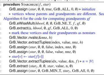
Algorithm 7Updating star memberships. Inputs: the parent vector f, the star vectorstar.Output: Updatedstarvector.

1: procedureStarcheck(f,star)

2: GrB assign(star,∅,∅, true, GrB ALL, 0,∅).initialize 3: .vertices whose parents and grandparents are different. See

Algorithm 6 for the code for computing grandparentsgf

4: GrB eWiseMult(hbool,∅,∅, GrB NE T,f,gf,∅) 5: GrB extract(h,hbool,∅,gf, GrB ALL, 0,∅)

6: .mark these vertices and their grandparents as nonstars 7: GrB Vector nvals(&nnz,h)

8: GrB Vector extractTuples(index, value, nnz,h) 9: GrB assign(star,∅,∅, false, index, nnz,∅) 10: GrB assign(star,∅,∅, false, value, nnz,∅) 11: .star[v]←star[f[v]]

12: GrB Vector extractTuples(idx, value, &n, f).n=|V| 13: GrB extract(starf,∅,∅,star, value, n,∅)

14: GrB assign(star,∅, GrB MIN T,starf, GrB All, 0,∅)

Table 1: The scope of using sparse vectors at different steps of LACC (does not apply to the first iteration).

Operation Operate on the subset of vertices in Conditional hooking Nonstars after unconditional hooking in the previous iteration Unconditional hooking Nonstars after conditional hooking Shortcut Nonstars after unconditional hooking Starcheck Nonstars after unconditional hooking

iterations. Hence Lemma 1 impacts all four steps of LACC. Since Lemma 1 does not apply to iteration 1, it has no influence in the first two iterations of LACC. Furthermore, a graph with a few components is not benefited significantly as most vertices will be active in almost every iteration.

Lemma 2. Unconditional hooking does not hook a star on an-other star [5, Theorem 2(a)].

Consequently, we can further sparsify unconditional hook-ing as was described in Algorithm 5. Even though uncondi-tional hooking can hook a star onto another star in the first iter-ation, we prevent it by removing conditionally hooked vertices from consideration in unconditional hooking.

According to Lemma1, only nonstar vertices after uncon-ditional hooking will remain active in subsequent iterations. Hence, only these vertices are processed in the shortcut and starcheck operations. Table1summarizes the subset of vertices used in different steps of our algorithm.

4.3. The FastSV algorithm using linear algebra

Algorithm8 describes the complete FastSV algorithm us-ing the GraphBLAS API. We maintain both the parent vector f and the grandparent vectorgf in each iteration. The hooking phase is similar to LACC’s conditional hooking phase, which

uses GrB mxv to identify for each u the with the minimum

gf[v] among all the edges{u,v}inE. The matrix multiplication A· f is parameterized with the same (Select2nd, min) semir-ing, and the output is stored in fn. Then, the stochastic hooking

Algorithm 8The linear algebra FastSV algorithm. Input: an adjacency matrixAand the parent vector f.Output: Updated

f. (NULL is denoted by∅) 1: procedureFastSV(A,f) 2: GrB Matrix nrows(&n,A)

3: GrB Vector dup(&gf,f).initial grandparent 4: GrB Vector dup(&dup,gf).duplication ofgf

5: GrB Vector extractTuples(index,value,&n,f)

6: Sel2ndMin←a (select2nd, Min) semiring

7: repeat

8: .Step 1: Hooking phase

9: GrB mxv(fn,∅,GrB MIN T,sel2ndMin,A,gf,∅) 10: GrB assign(f,∅,GrB MIN T,fn,value,n,∅) 11: GrB eWiseMult(f,∅,∅,GrB MIN T,f,fn,∅) 12: .Step 2: Shortcutting

13: GrB eWiseMult(f,∅,∅,GrB MIN T,f,gf,∅) 14: .Step 3: Calculate grandparents

15: GrB Vector extractTuples(index,value,&n,f) 16: GrB extract(gf,∅,∅,f,value,n,∅)

17: .Step 4: Check termination

18: GrB eWiseMult(diff,∅,∅,GxB ISNE T,dup,gf,∅) 19: GrB reduce(&sum,∅,Add,diff,∅)

20: GrB assign(dup,∅,∅,gf,GrB ALL,0,∅)) 21: untilsum=0

f[f[u]] ← fn[u] is implemented by theGrB assign function

in line 10, which assigns the entries of fn into the specified

locations of vector f, and the indicesvalueis extracted from the vector f in either line 5 before the first iteration or line 15 from the previous iteration. Next, the aggressive hooking f[u] ← fn[u] is implemented by an element-wise

multiplica-tion f ← min(f,fn) in line 11, and the shortcutting operation f ←min(f,gf) is implemented in the same way in line 13. We recalculate the grandparent vectorgf[u]← f[f[u]] in line 15-16, and in the end of each iteration, we calculate the number of modified entries ingf in line 18 - 19 to check whether the algorithm has converged or not. A copy ofgf is stored in the vectordupfor determining the termination in the next iteration.

5. Parallel implementations of LACC and FastSV

In the previous section, we described two connected compo-nent algorithms LACC and FastSV using linear algebraic oper-ations. Given libraries with parallel implementations of those linear algebraic operations, we can easily implement LACC and FastSV. In this section, we describe the implementations of LACC and FastSV using a shared-memory and a memory parallel library. We primarily focus on distributed-memory implementation and discuss detailed computation and communication complexity.

5.1. Parallel LACC and FastSV for shared memory platforms Currently, the SuiteSparse:GraphBLAS library4 provides a full implementation of the GraphBLAS C API with

the OpenMP parallelism. Therefore, algorithms described in Section 4 can be directly implemented in the SuiteS-parse:GraphBLAS library. In the earlier conference version of this work, we implemented LACC and FastSV using SuiteS-parse:GraphBLAS just to test the correctness of the presented algorithms with respect to the GraphBLAS API. In this paper, we show detailed shared-memory performance of LACC and FastSV’s SuiteSparse:GraphBLAS implementation in Section 6.3. Our SuiteSparse:GraphBLAS implementation is commit-ted to the LAGraph Library.

5.2. Parallel LACC and FastSV for distributed-memory plat-forms

We use the CombBLAS library [13] to implement LACC and FastSV for distributed-memory platforms. Since Comb-BLAS does not directly support the masking operations, we use element-wise filtering after performing an operation when masking is needed.

CombBLAS distributes its sparse matrices on a 2Dpr×pc

processor grid. ProcessorP(i,j) stores the submatrixAi jof

di-mensions (m/pr)×(n/pc) in its local memory. CombBLAS

uses the doubly compressed sparse columns (DCSC) format to store its local submatrices for scalability, and uses a vector of

{index, value}pairs for storing sparse vectors. Vectors are also distributed on the same 2D processor grid in a way that en-sures that processor boundaries aligned for vector and matrix elements during multiplication.

5.3. Parallel complexity of linear-algebraic operations used in LACC and FastSV

We explain the parallel complexity of LACC and FastSV with respect to the GraphBLAS operations which LACC and FastSV depend upon. Here, we measure communication by the number ofwordsmoved (W) and the number ofmessagessent (S). The cost of communicating a lengthmmessage isα+βm whereαis the latency andβis the inverse bandwidth, both de-fined relative to the cost of a single arithmetic operation. Hence, an algorithm that performs F arithmetic operations, sends S messages, and movesWwords takesT =F+βW+αS time.

Our GrB mxv internally maps to either a sparse-matrix

dense-vector multiplication (SpMV) for the few early iter-ations when most vertices are active or to a sparse-matrix sparse-vector multiplication (SpMSpV) for subsequent itera-tions. Given the 2D distribution CombBLAS employs, both functions require two steps of communication: first within column processor groups, and second within row processor groups. The first stage of communication is a gather operation to collect the missing pieces of the vector elements needed for the local multiplication and the second one is a reduce-scatter operation to redistribute the result to the final vector. Both stages can be implemented to take advantage of vector spar-sity. In fact, there is exciting research on the sparse reduction problem [35,36]. We found that a simple allgather is the most performant for both SpMV and SpMSpV for the first stage in our case. For the reduce-scatter phase, SpMV uses a simple re-duction within a loop (i.e. one for each processor in the row

group) whereas SpMSpV uses an irregular all-to-all operation followed by a local merge.

Assuming a square processor grid pc=pr= √

p and a load balanced matrix withmnonzeros, one SpMV iteration costs

TSpMV=O m p +β n √ p √ p−1 √ p +lg √ p+α √ p+lg√p using standard MPI implementations [37].

For the SpMSpV case, let the density of input vector be f and the unreduced output vector beg. While f is always less than or equal to 1, this is not necessarily the case forgbecause the number of nonzeros in the unreduced vector can be larger thann. If that is the case, we resort to a dense reduce-scatter operation similar to the one employed by SpMV. Hence, when we writeg, we mean min(g,1). Assuming that the nonzeros in vectors are i.i.d. distributed, the cost of SpMSpV is

TSpMSpV=O m f p +β n f+ng √ p √ p−1 √ p +α √ p+lg√p. Vector variants of GrB extract andGrB assign are fairly general functions that can be exploited to perform very diff er-ent computations. That being said, our use of them are suffi -ciently constrained that we can perform a reasonably tight anal-ysis. The cost ofGrB extractprimarily depends on the num-bers of nonzeros in the output vectorw. In contrast, the cost of

GrB assignprimarily depends on the numbers of nonzeros in

the input vectoru. They both use the irregular all-to-all primi-tive for communication. With similar load balance assumptions as before, which can be theoretically achieved using a cyclic vector distribution, the cost ofGrB assignis:

T_assign=O nnz(u)

p +β

nnz(u)

p +α(p−1) .

The cost of GrB extract is identical except that nnz(u) is replaced bynnz(w). Remember thatnnz(u),nnz(w)≤n.

In practice, we achieve high performance in all-to-all oper-ations by employing other optimizoper-ations to CombBLAS’ block distributed vectors, described in Section5.4, instead of using a cyclic distribution.

Despite our sparsity aware analysis of individual primitives, we could not prove bounds on aggregate sparsity across all it-erations. We can, however, still provide an overall complex-ity assuming the worst casennz(u),nnz(w) = n and f,g = 1. Given that there are a constant number of calls to GraphBLAS primitives in each iteration and the algorithm converges in lg(n) iterations, LACC’s sparsity-agnostic parallel cost is:

TLACC=O mlg(n) p +β nlg(n) lg(√p) √ p +α(p−1) lg(n) .

Each iteration of FastSV (Algorithm8) has the same asymp-totic complexity as LACC. In practice, an iteration of FastSV can run faster because of its simplicity. For example, FastSV

0 20,000 40,000 60,000 80,000 100,000 120,000 P0 P2 P4 P6 P8 P10 P12 P14 Nu m be r of r eq ue st s MPI processes Iteration 1 0 5,000 10,000 15,000 20,000 25,000 30,000 P0 P2 P4 P6 Nu m be r of r eq ue st s MPI processes Iteration 7

Figure 3: Number of requests received by every process when accessing grand-parents. We show iteration 1 and 7 when running LACC with 16 processes. Only even numbered processes are labeled on the x-axis. Lower ranked pro-cesses receive more requests than higher ranked process in all iterations. Later iterations are more imbalanced than earlier iterations.

needs one SpMV operation, where as LACC needs two Sp-MVs. However, FastSV can take O(n) iterations in the worst case. Hence, FastSV’s parallel cost is:

TF_astSV=O mn p +β n2lg(√p) √ p +α(p−1)n .

Because of our aggressive hooking strategies, FastSV needed approximately the same number of iterations as needed by LACC in all problems we experimented in this paper. Con-sequently, FastSV runs faster than LACC in practice despite its higher asymptotic complexity.

5.4. Load balancing and communication efficiency

In CombBLAS, we randomly permute the rows and columns of the adjacency matrix, resulting in load-balanced distribution of the matrix and associated dense vectors. Hence,

GrB mxv is a load-balanced operation both in terms of

com-putation and communication. However, GrB assign and

GrB extract can be highly imbalanced when a vector is

in-dexed by parents. For example, Figure 3 shows the number of requests received by every process when extracting grand-parents usingGrB extractin two different iterations of LACC. This imbalance is caused primarily by the conditional hooking (via the (select2nd, min) semiring), where parents have smaller ids than their children. Since CombBLAS employs a block distribution of vectors, lower-ranked processes receive more data than higher-ranked processes in all-to-all communication, which may result in poor performance. Many of these received requests need to access the same data at the recipient process, incurring redundant data access and communication.

To alleviate this problem with highly skewed all-to-all com-munication, we broadcast entries from few low-ranked pro-cesses and then remove those propro-cesses from all-to-all collec-tive operations. If a processor receiveshtimes more requests than the total number of elements it has, it broadcasts its lo-cal part of a vector rather than participating in an all-to-all col-lective call. Here,his a system-dependent tunable parameter. If more than one process broadcasts data in an iteration, we use nonblockingMPI Ibcastso that they can proceed indepen-dently.

We also used two more optimizations to make all-to-all communication more efficient. First, when data is highly imbal-anced as shown in Figure3, we noticed that all-to-all operations

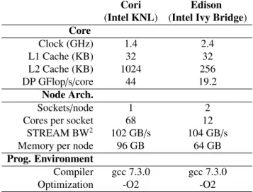
Table 2: Overview of evaluation platforms.2_{Memory bandwidth is measured} using the STREAM copy benchmark per node.

Cori Edison

(Intel KNL) (Intel Ivy Bridge) Core Clock (GHz) 1.4 2.4 L1 Cache (KB) 32 32 L2 Cache (KB) 1024 256 DP GFlop/s/core 44 19.2 Node Arch. Sockets/node 1 2

Cores per socket 68 12

STREAM BW2 102 GB/s 104 GB/s Memory per node 96 GB 64 GB Prog. Environment

Compiler gcc 7.3.0 gcc 7.3.0

Optimization -O2 -O2

in Cray’s MPI library at NERSC are not scaling beyond 1024 MPI ranks. A possible reason could be the use of the pairwise-exchange algorithm that hasα(p−1) latency cost [37]. Hence, we replace allMPI Alltoallvcalls with a hypercube-based im-plementation by Sundar et al. [38], which hasαlog(p) latency cost. Second, in iteration 7 of Figure3, processes 7-15 have no data to communicate. In that case (after P0 broadcasts its data), we use a sparse variant of all-to-all implementation [38], where only P1-P5 exchange data. All of these optimizations made our implementations ofGrB assign andGrB extract highly scal-able as seen in Figure9.

6. Results

6.1. Evaluation platforms

Shared-memory platform. We evaluate the shared-memory performance of LACC, FastSV, and other CC algo-rithms on an Amazon AWS r5.8xlarge instance with Intel Xeon Platinum 8000 CPU (3.1GHz, 249G memory). We use up to 16 threads in our shared-memory experiments.

Distributed-memory platform. Distributed-memory ex-periments were conducted on NERSC Edison and Cori KNL supercomputers as described in Table2. Even though the Edi-son supercomputer is not longer in service, we keep results from Edison to keep this paper consistent with the preceding conference paper [11]. Our distributed-memory implementa-tions uses OpenMP for multithreaded execution within an MPI process. In our experiments, we only used square process grids because rectangular grids are not supported in Comb-BLAS [13]. When p cores are allocated for an experiment, we create a pp/t× pp/tprocess grid wheret is the number of threads per process. All of our experiments used 16 and 6 threads per MPI process on Cori and Edison, respectively. In our hybrid OpenMP-MPI implementation, all MPI processes perform local computation followed by synchronized commu-nication rounds. Only one thread in every process makes MPI calls in the communication rounds.

Table 3: Test problems used to evaluate parallel connected component algorithms. We report directed edges because the symmetric adjacency matrices are stored in LACC. We cite the sources from where we obtained the graphs.

Graph Vertices Directed edges Components Description

archaea 1.64M 204.79M 59,794 archaea protein-similarity network [8] queen 4147 4.15M 329.50M 1 3D structural problem [39]

eukarya 3.23M 359.74M 164,156 eukarya protein-similarity network [8] uk-2002 18.48M 529.44M 1,990 2002 web crawl of .uk domain [39]

M3 531M 1.047B 7.6M Soil metagenomic data [10]

twitter7 41.65M 2.405B 1 twitter follower network [39] sk-2005 50.64M 3.639B 45 2005 web crawl of .sk domain [39]

MOLIERE 2016 30.22M 6.677B 4,457 automatic biomedical hypothesis generation system [39] Metaclust50 282.2M 42.79B 15.98M similarities of proteins in Metaclust50 [8]

iso m100 68.48M 67.16B 1.35M similarities of proteins in IMG isolate genomes [8]

6.2. Test problems

Table 3 describes ten test problems used in our experi-ments. These graphs contain a wide range of connected compo-nents and cover a broad spectrum of applications. The protein-similarity networks are generated from the IMG database at the Joint Genome Institute and are publicly available as part of the HipMCL software [8].

6.3. Shared-memory performance

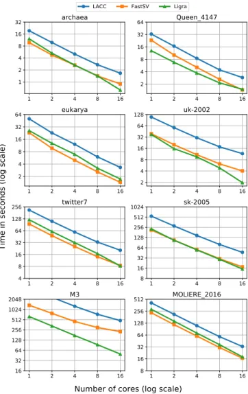
The shared-memory implementations of LACC and FastSV can be directly obtained from SuiteSparse:GraphBLAS, a multi-threaded implementation of the GraphBLAS standard. We compare them with a popular shared-memory graph pro-cessing framework Ligra [40], which implements the propa-gation algorithm using parallel breadth-first search (BFS). We chose not to compare with other hand-tuned connected compo-nent codes because our objective is to show that linear-algebraic CC algorithms are competitive to popular graph processing frameworks such as Ligra. As mentioned before, our shared-memory experiments are conducted on an Intel Xeon Platinum 8000 CPU with up to 16 threads.

Figure4shows the shared-memory performance of LACC and FastSV implemented using SuiteSparse:GraphBLAS and Ligra’s CC implementation. Here, we only experimented with the first eight graphs from Table3because the last two graphs did not fit on the memory of our single node server. LACC and FastSV are originally designed for reducing the commu-nication cost on distributed-memory, but their shared-memory implementations are also competitive with Ligra. Especially, the simplicity of FastSV makes it efficient on multithreaded en-vironments. For six out of eight graphs in Figure4, FastSV’s runtime is within 17% of Ligra’s CC implementation. This re-sults indicates that SuiteSparse:GraphBLAS has scalable im-plementations of linear algebraic operations that we used in our algorithms. However, for some problems like the very sparse M3 graph, FastSV can be much slower than Ligra. M3 is an extremely sparse graph and it is possible that SuiteS-parse:GraphBLAS is not well optimized for these type of very sparse graphs (especially if we use SpMV in every iteration of the SV algorithm). By contrast, Ligra’s implementation care-fully handles the BFS’s frontier so that it does not span the

1 2 4 8 16 1 2 4 8 16 32 archaea 1 2 4 8 16 2 4 8 16 32 64 Queen_4147 1 2 4 8 16 2 4 8 16 32 64 eukarya 1 2 4 8 16 2 4 8 16 32 64 128 uk-2002 1 2 4 8 16 4 8 16 32 64 128 256 twitter7 1 2 4 8 16 8 16 32 64 128 256 512 1024 sk-2005 1 2 4 8 16 16 32 64 128 256 512 1024 2048 M3 1 2 4 8 16 8 16 32 64 128 256 512 MOLIERE_2016

Time in seconds (log scale)

Number of cores (log scale)

---LACC FastSV Ligra

Figure 4: Scalability of LACC, FastSV and Ligra with regarding to the number of threads on eight small datasets using 16 threads.

whole vertex set in every iteration. Another reason for Ligra’s superior performance on very sparse graph might be due to its direction optimization. TheGrB mxv function within SuiteS-parse:GraphBLAS does not automatically implement this

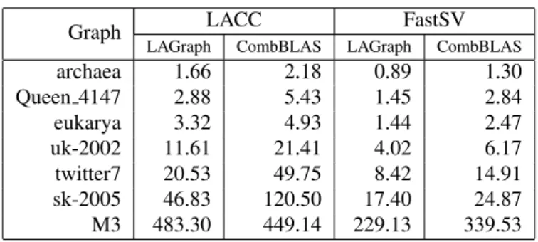
fea-Table 4: Comparison of the runtime of CombBLAS and LAGraph (developed on top of SuiteSparse:GraphBLAS) using 16 threads (in seconds).

Graph LACC FastSV

LAGraph CombBLAS LAGraph CombBLAS

archaea 1.66 2.18 0.89 1.30 Queen 4147 2.88 5.43 1.45 2.84 eukarya 3.32 4.93 1.44 2.47 uk-2002 11.61 21.41 4.02 6.17 twitter7 20.53 49.75 8.42 14.91 sk-2005 46.83 120.50 17.40 24.87 M3 483.30 449.14 229.13 339.53

ture that would switch search direction depending on the spar-sity of input and output vectors. This feature, however, is imple-mented in GraphBLAST [41] and we expect it to be available soon in other GraphBLAS-inspired libraries.

LACC is approximately 2×to 3×slower than FastSV and Ligra. This is primarily due to LACC’s use of two SpMV oper-ations (that is theGrB mxvfunction) needed in the conditional and unconditional hooking (as opposed to one SpMV needed by FastSV). Note that for most graphs, SpMV is the most ex-pensive operation, since it needs to traverse all edges of the graph. Therefore, each iteration of LACC is about 2×slower than a FastSV iteration that uses SpMV only once in its stochas-tic hooking.

Figure4demonstrates that all three shared-memory imple-mentations scale almost linearly up to 16 threads. On aver-age, LACC, FastSV and Ligra achieves 11.4×, 12.3×, 15.09×

speedup on 16 threads with respect to their sequential runtimes. Overall, we highlight the fact that connected component algo-rithms implemented using linear-algebraic operations can at-tain high performance on shared memory platforms. This per-formance is comparable to the state-of-the-art shared-memory platforms. However, true benefits of linear-algebraic operations can be realized in the distributed-memory systems, as we will demonstrate in the next few sections.

6.4. Single node performance of LACC and FastSV when im-plemented using SuiteSparse:GraphBLAS and CombBLAS Even though CombBLAS is designed for distributed-memory platforms, it can also attain good performance on a single node. Since we implemented LACC and FastSV us-ing both SuiteSparse:GraphBLAS and CombBLAS, we com-pare their performance on a single node with multicore pro-cessors. For this experiment, we used the same configura-tion used in the experiments in Secconfigura-tion 6.3.For CombBLAS, we always use a 4×4 process grid with each process having one thread during the computation. Table4 presents the run-time of LACC and FastSV implemented in CombBLAS and SuiteSparse:GraphBLAS using 16 threads. We only show re-sults for graphs that fit in the memory of a node. On all the seven graphs, we observe that CombBLAS is on average 1.78×

and 1.62×slower than GraphBLAS for LACC and FastSV, re-spectively. This slowdown of CombBLAS is possibly due its distributed-memory overheads such as MPI communication and

buffer copies. Therefore, we observe that CombBLAS itself is an efficient linear algebraic library on shared-memory, and the extra overhead is worth paying to obtain the extraordinary scal-ability and high-performance on large supercomputers. 6.5. Performance of LACC and FastSV in distributed-memory

As mentioned before, we implemented distributed mem-ory LACC and FastSV using the CombBLAS library. Here, we compare the performance of distributed LACC and FastSV with ParConnect [10], the state-of-the art algorithm prior to our work. Similar to our algorithms, ParConnect also depends on CombBLAS; hence, both of them require a square process grid. Since ParConnect does not use multithreading, we place one MPI process per core in ParConnect experiments.

Figure 5 shows the performance of LACC and ParCon-nect with the smaller eight test problems on Edison (we did not show FastSV on Edison because Edison went out of ser-vice when FastSV was developed). Both LACC and ParCon-nect scale well up to 6144 cores (256 nodes), but LACC runs faster than ParConnect on all concurrencies. On 256 nodes, LACC is 5.1×faster than ParConnect on average (min 1.2×, max 12.6×). LACC is expected to perform better when a graph has many connected components because, for these graphs, we have better opportunities to employ sparse operations. Conse-quently, LACC performs the best for archaea and eukarya. For M3, LACC performs comparably to ParConnect, which will be explained in detail in Section6.7.

The relative performance of LACC and ParConnect on Cori KNL is similar to Edison as can be seen in Figure6. We ad-ditionally show the strong scaling of FastSV, which is gener-ally faster than both LACC and ParConnect. As with Edison, LACC outperforms ParConnect on all core counts on Cori for all graphs except M3, for which the performance is compara-ble. FastSV is faster than LACC because of the former using only one SpMV operation per iteration. However, we also ob-verse that LACC scales slightly better than FastSV. For exam-ple, in Figure6, the gap between LACC and FastSV decreases as we increase cores for eukarya and twitter7. Better scala-bility of LACC is due to its use of sparse operations which in turn reduce the communication on high concurrency. Generally, all three connected component algorithms ran faster on Edison than Cori given the same number of nodes. This behavior is common for sparse graph manipulations where few faster cores (e.g., Intel Ivy Bridge on Edison) are more beneficial than more slower cores (e.g., KNL on Cori) [42].

6.6. Performance of CC algorithms for bigger graphs

In the previous section, we presented results for smaller graphs, each of which can be stored in less than 150GB mem-ory (ignoring MPI overheads). It is often possible to store these graphs on a shared-memory server and compute connect components using an efficient shared-memory algorithm [33]. However, the last two graphs in Table3need more than 1TB memory, requiring distributed-memory processing. We show the performance of LACC, FastSV and ParConenct for these big graphs in Figure7. We observed that LACC and FastSV

Number of cores (log scale) Time in sec onds (log sc ale) 24 96 384 1536 6144 1 4 16 64 archaea 24 96 384 1536 6144 1 4 16 64 256 1024 uk-2002 24 96 384 1536 6144 2 8 32 128 queen-4147 24 96 384 1536 6144 1 4 16 64 256 1024 eukarya 384 1536 6144 1 4 16 MOLIERE_2016 96 384 1536 6144 1 4 16 twitter7 96 384 1536 6144 1 4 16 64 sk-2005 LACC ParConnect 384 1536 6144 8 16 32 64 M3

Figure 5: Strong scaling of LACC and ParConnect on Edison on (up to 6144 cores on 256 nodes). LACC uses 4 MPI processes per node and ParConnect uses 24 MPI processes per node.

Number of cores (log scale)

Time in sec onds (log sc ale) 64 256 1024 4096 16384 2 8 32 128 archaea 64 256 1024 4096 16384 1 4 16 64 256 uk-2002 64 256 1024 4096 16384 2 8 32 128 queen-4147 64 256 1024 4096 16384 1 4 16 64 256 eukarya 256 1024 4096 16384 8 32 128 M3 256 1024 4096 16384 8 32 128 sk-2005 256 1024 4096 16384 8 32 twitter7 256 1024 4096 16384 2 8 32 128 MOLIERE_2016 LACC ParConnect FastSV

Figure 6: Strong scaling of LACC and ParConnect on Cori KNL (up to 16,384 cores on 256 nodes). LACC uses 4 MPI processes per node and ParConnect uses 64 MPI processes per node. Graphs with large numbers of connected components are shown.

continue scaling to 4096 nodes (262,144 cores) on Cori and computes connected components in these large networks in less than 16 seconds. By contrast, ParConnect does not scale be-yond 16,384 cores for these two graphs. One reason of Par-Connect not performing well on high core counts could be its reliance on flat MPI. On 262,144 cores, ParConnect cre-ates 262,144 MPI processes and needs more than two hours to find connected components. Once again, we observe that LACC scales slightly better than FastSV on high concurrency. The remarkable ability of LACC and FastSV to process graphs with tens of billions of edges on hundreds of thousands cores makes it well suited for large-scale applications such as high-performance Markov clustering [8]. We will discuss this in more detail in Section6.8.

6.7. Understanding the performance of LACC

We now explore different features of LACC and describe why it achieves good performance for most of the test graphs5_.

(a) Number of active vertices (vector sparsity). When fewer vertices remain active in an iteration, LACC performs less work and communicate less data. Hence, identifying and eliminating converged forests boost the performance of LACC significantly. In our GraphBLAS-style implementation, this translates into sparser vectors, which impacts the performance

ofGrB mxv,GrB assign, andGrB extract. However, LACC

can take advantage of the vector sparsity only if the input graph 5_{Here, we only discuss detail performance of LACC since this paper is an} extension of the LACC paper [11]. Detailed performance of FastSV can be found in [12].

4096 16384 65536 262144 Number of Cores 4 16 64 256 1024 4096 16384 Time (sec) Metaclust50 (LACC) iso_m100 (LACC) Metaclust50 (ParConnect) iso_m100 (ParConnect) Metaclust50 (FastSV) iso_m100 (FastSV)

Figure 7: Performance of LACC and ParConnect with two large protein-similarity networks on Cori KNL (up to 262,144 cores on 4096 nodes). LACC and ParConnect use 4 and 64 MPI processes per node, respectively. While LACC scales to 262,144 cores, ParConnect stopped scaling at this extreme scale. ParConnect ran out of memory on 64 nodes.

0% 20% 40% 60% 80% 100%

archaea eukarya M3 Metaclust50 iso_m100

% co nv er ge d ve rt ic es

Figure 8: Percentage of vertices in converged connected components at dif-ferent iterations of LACC. For every graph, iterations are shown incrementally from left to right.

has a large number of connected components. To demonstrate this, Figure8plots the percentage of vertices in converged com-ponents for five graphs with the highest number of comcom-ponents. We observe that a significant fraction of vertices becomes inac-tive after few iterations. Hence, LACC is expected to perform better (both sequential and parallel cases) for these graphs. Fig-ure5and Figure7confirm this expectation except for M3. For M3, LACC needs 11 iterations, eight of which have less than 5% converged vertices. Hence, LACC can not take advantage of vector sparsity in most of the iterations, which can partially explains the observed performance of LACC on the M3 graph. For a connected graph, LACC can not take advantage of vector sparsity at all.

(b) Sparsity of the input graph. The sparsity of the input graph also impacts the performance and scalability of LACC. When a dense vector is used, the computational cost

of GrB mxv is O(m), while all other operations take O(n)

time. Since GrB assign andGrB extract may communicate O(n) data, the computation to communication ratio of LACC is O(m/n). For very sparse graphs similar to M3, communi-cation starts to dominate the overall runtime, affecting the per-formance of our GraphBLAS kernels. High graph sparsity and

lack of vector sparsity in most iterations play roles in the per-formance of LACC on the M3 graph. By contrast, queen 4147 (with average degree of 82) is denser than M3. Consequently, LACC performs much better on queen 4147 despite it having a single component.

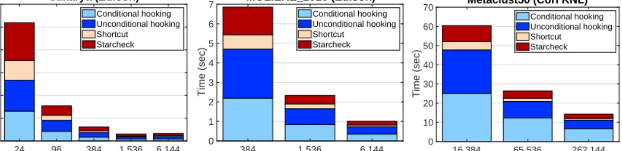
(c) Scalability of different parts of LACC.Figure9shows the performance breakdown of LACC for three representative graphs, where all four parts of LACC scale well on Edison and Cori. For smaller graphs like eukarya, LACC stops scaling after 64 nodes (1,536 cores) because of the relatively high commu-nication overhead on high concurrency. We also observe that conditional hooking is usually more expensive than uncondi-tional hooking because the latter can utilize addiuncondi-tional vector sparsity as shown in Lemma2. Finally, our adaptive communi-cation scheme discussed in Section5.4makes the shortcut and starcheck operations highly scalable.

6.8. Performance of LACC when used in Markov clustering As discussed in the introduction, finding connected com-ponents is an important step in the popular Markov cluster-ing algorithm. LACC is already incorporated with HipMCL where LACC can be 3288×faster (on 1024 nodes of Edison) than the shared-memory parallel connected component algo-rithm used in the original MCL software [1]. HipMCL is an ongoing project with an aim to scale to upcoming exascale sys-tems and cluster more than 50B proteins in the IMG database (https://img.jgi.doe.gov/). A massively-parallel LACC boosts HipMCL’s performance and helps us cluster massive biological networks with billions of vertices and trillions of edges.

7. Opportunities and limitations of linear-algebraic CC al-gorithms

The primary advantage of linear-algebraic CC algorithms like LACC and FastSV is their reliance on off-the-shelf func-tions from high-performance libraries like CombBLAS and SuiteSparse:GraphBLAS. As a result, we were able to imple-ment LACC and FastSV rapidly after designing them in the language of linear algebra. This paper demonstrated the eff ec-tiveness of our approach where LACC and FastSV scaled to hundreds of thousands of cores with the support of the highly-optimized CombBLAS library.

Even though LACC and FastSV achieve remarkable scala-bility, it is certainly possible to develop highly optimized hand-tuned codes that run faster than LACC and FastSV. Notably, customized CC algorithms perform well on shared-memory platforms using improved data locality and sampling tech-niques. For example, a recent algorithm called Afforest [33] used sampling to develop a shared-memory parallel CC algo-rithm. The implementation of Afforest in the GAP bench-mark [43] runs up to 5×faster than the shared-memory FastSV code implemented on top of SuiteSparse:GraphBLAS. Sim-ilarly, the iSpan algorithm [44] uses various asynchronous schemes and direction-optimized BFS to find connected com-ponents quickly and can run faster than our algorithms on mul-ticore processors. Recently, Dhulipala et al. [45] developed a

eukarya (Edison) 24 96 384 1,536 6,144 Number of Cores 0 1 2 3 4 5 6 Time (sec) Conditional hooking Unconditional hooking Shortcut Starcheck MOLIERE_2016 (Edison) 384 1,536 6,144 Number of Cores 0 1 2 3 4 5 6 7 Time (sec) Conditional hooking Unconditional hooking Shortcut Starcheck Metaclust50 (Cori KNL) 16,384 65,536 262,144 Number of Cores 0 10 20 30 40 50 60 70 Time (sec) Conditional hooking Unconditional hooking Shortcut Starcheck

Figure 9: Performance breakdown of LACC for three representative graphs.

class of shared-memory parallel graph algorithms that achieve state-of-the-art performance on multicore servers with large memory. Their CC algorithm is based on a prior work [25] where they compared with Ligra’s direction-optimized CC im-plementation. Since FastSV can be up to 2× slower than Ligra’s CC implementation (see Fig. 4), it can be at most 4× slower than the CC algorithm reported by Dhulipala et al. [45]. Overall, it is expected that customized shared-memory codes [33, 44, 45] would perform better than our algorithms based on general-purpose linear algebra libraries.

LACC and FastSV achieve the state-of-the-art performance in distributed memory. This performance is achieved by us-ing highly-optimized distributed primitives available in Comb-BLAS. However, on a single shared-memory platform, LACC and FastSV implemented on CombBLAS are up to 2×slower than their implementations on SuiteSparse:GraphBLAS (see Table4). This slowdown is observed due to the overheads in CombBLAS which is optimized for distributed-memory plat-forms. Highly-scalable algorithms like LACC and FastSV are especially valuable when the graph does not fit in the memory of a single node or when the graph is already distributed as part of another application such as HipMCL [8].

It is generally hard to relate the performance of a distributed algorithm to the input graph characteristics. In our experiments, we observed various performance gains with different graphs. Generally, LACC and FastSV perform better for graphs with a large number of connected components. For example, on a low-diameter graph with a single connected component, a BFS-based algorithm is expected to perform better than LACC and FastSV. In a graph with many connected components, LACC avoids already-found connected components in subsequent it-erations by using sparse vectors. This approach is only useful when a sizable fraction of connected components is found in early iterations (see Fig.8). However, it is often not possible to predict the number of components or the rate of component dis-coveries in advance from some summary statistics of the graph. Hence, we did not find a clear correlation between the perfor-mance of LACC and FastSV and the input graphs.

8. Conclusions

We present two distributed-memory connected component algorithms LACC and FastSV that are implemented using

sparse linear algebra and are based on the Shiloach-Vishkin algorithm. Both algorithms achieve unprecedented scalability to 4K nodes (262K cores) of a Cray XC40 supercomputer and outperforms previous state-of-the-art by a significant margin. There are three key reasons for the observed performance: (1) our algorithms rely on linear algebraic kernels that are highly optimized for distributed memory graph analysis, (2) whenever possible, our algorithms employ sparse vectors in the hooking, shortcutting and star finding steps, eliminating redundant com-putation and communication, and (3) our algorithms detect im-balanced collective communication patterns inherent in the CC algorithm and remove them with customized all-to-all opera-tions.

Extreme scalability achieved by linear-algebraic connected component algorithms such as LACC and FastSV can boost the performance of many large-scale applications. Metagenome as-sembly and protein clustering are two such applications that compute connected components in graphs with hundreds of bil-lions or even trilbil-lions of edges on hundreds of thousands of cores.

The use of sparsity (Lemma 1 and 2 in Section4) is a prop-erty of the Awerbuch-Shiloach algorithm and can be applied to any Awerbuch-Shiloach implementation. The customized communications are related to the way CombBLAS distributes sparse matrices and vectors. As future work, we plan to im-prove our vector operations so that they can avoid communica-tion hot spots and work better on very sparse graphs similar to the M3 graph in Table3. Using cyclic distributions of vectors, instead of the current block distribution used in CombBLAS, is one possible approach to distribute load more evenly and make LACC even more scalable.

In terms of reducing the number of actual operations per-formed, we plan to utilize the automatic direction optimization feature of GraphBLAST [41] in order to be competitive with Ligra on very sparse graphs as well. Porting our code to Graph-BLAST will also enable LACC to seamlessly run on GPUs.

9. Acknowledgments

Partial funding for AA was provided by the Indiana Univer-sity Grand Challenge Precision Health Initiative. AB was sup-ported in part by the Applied Mathematics program of the DOE