Assessing Invariance of Factor Structures and Polytomous Item Response Model Parameter Estimates

(1)

ASSESSING INVARIANCE OF FACTOR STRUCTURES AND POLYTOMOUS ITEM RESPONSE MODEL PARAMETER ESTIMATES

A Dissertation by

JENNIFER MCGEE REYES

Submitted to the Office of Graduate Studies of Texas A&M University

in partial fulfillment of the requirements for the degree of

DOCTOR OF PHILOSOPHY

December 2010

(2)

ASSESSING INVARIANCE OF FACTOR STRUCTURES AND POLYTOMOUS ITEM RESPONSE MODEL PARAMETER ESTIMATES

A Dissertation by

JENNIFER MCGEE REYES

Submitted to the Office of Graduate Studies of Texas A&M University

in partial fulfillment of the requirements for the degree of

DOCTOR OF PHILOSOPHY

Approved by:

Chair of Committee, Bruce Thompson Committee Members, David J. Martin

Michael Speed

Victor L. Willson Head of Department, Victor L. Willson

December 2010

(3)

ABSTRACT

Assessing Invariance of Factor Structures and Polytomous Item Response Model Parameter Estimates.

(December 2010)

Jennifer McGee Reyes, B.A., Syracuse University; M.A., University of Houston – Clear Lake Chair of Advisory Committee: Dr. Bruce Thompson

The purpose of the present study was to examine the invariance of the factor structure and item response model parameter estimates obtained from a set of 27 items

selected from the 2002 and 2003 forms of Your First College Year (YFCY). The first major research question of the

present study was: How similar/invariant are the factor structures obtained from two datasets (i.e., identical items, different people)? The first research question was addressed in two parts: (1) Exploring factor structures using the YFCY02 dataset; and (2) Assessing factorial invariance using the YFCY02 and YFCY03 datasets.

After using exploratory and confirmatory and factor analysis for ordered data, a four-factor model using 20 items was selected based on acceptable model fit for the

(4)

YFCY02 and YFCY03 datasets. The four factors (constructs) obtained from the final model were: Overall Satisfaction, Social Agency, Social Self Concept, and Academic Skills. To assess factorial invariance, partial and full factorial invariance were examined. The four-factor model fit both datasets equally well, meeting the criteria for partial and full measurement invariance.

The second major research question of the present study was: How similar/invariant are person and item parameter estimates obtained from two different datasets (i.e., identical items, different people) for the

homogenous graded response model (Samejima, 1969) and the partial credit model (Masters, 1982)?

To evaluate measurement invariance using IRT methods, the item discrimination and item difficulty parameters obtained from the GRM need to be equivalent across

datasets. The YFCY02 and YFCY03 GRM item discrimination parameters (slope) correlation was 0.828. The YFCY02 and YFCY03 GRM item difficulty parameters (location)

correlation was 0.716. The correlations and scatter plots indicated that the item discrimination parameter estimates were more invariant than the item difficulty parameter estimates across the YFCY02 and YFCY03 datasets.

(5)

ACKNOWLEDGEMENTS

I am indebted to the Higher Education Research Institute (HERI) at the University of California, Los Angeles (UCLA) for providing the data for the present research at no cost.

I am so grateful to Carol Wagner and Kristie Stramaski, graduate advisors in the Department of

Educational Psychology, for their reassuring and capable guidance throughout my years in the program.

Thank you to my committee members, Dave Martin, Michael Speed, Vic Willson, and Bruce Thompson, for your time, patience, and support in the classroom and throughout the course of my dissertation.

In the classroom and throughout the dissertation, I have been encouraged by classmates, Colleen Cook and Troy Courville, and my colleagues in Student Life Studies.

Finally, thank you to my friends and family: Merna, Roemer, my mom and dad, Hema, and Joel. They always

believed in me and knew when to ask and, when not to ask, “How is the paper coming?”

(6)

TABLE OF CONTENTS Page ABSTRACT... iii ACKNOWLEDGEMENTS... v TABLE OF CONTENTS... vi LIST OF FIGURES... ix

LIST OF TABLES... xiii

CHAPTER I INTRODUCTION... 1

Statement of the Problem ... 12

Purpose of the Study... 12

Research Questions... 12

Delimitation... 13

Contents of the Present Study... 13

II LITERATURE REVIEW... 14

Measurement Invariance... 14

Fundamental Concepts of IRT... 22

Adjacent Category Models... 26

Cumulative Probability Models... 32

Parameter Estimation... 35

Parameter Invariance... 43

Item Information Functions... 47

Test Information Functions... 49

Assessing Model-Data Fit... 50

Comparing Polytomous Item Response Models for Ordered Data... 52

(7)

CHAPTER Page

III METHOD... 67

Contributions of Present Study... 67

Data Source... 68

Research Question 1: Factorial Invariance... 70

Research Question 2: Assessing IRT Parameter Invariance... 73

Assessing Measurement Invariance... 77

IV RESULTS... 78

Descriptive Statistics... 78

Research Question 1: Factorial Invariance... 100

Interpreting and Naming Factors... 121

Assessing Factorial Invariance... 123

Research Question 2: Assessing IRT Parameter Invariance... 130

Summary of GRM and PCM Model Fit Assessment... 238

Parameter Invariance of IRT Estimates... 246

Measurement Invariance Using IRT Methods... 259

Ancillary Analysis... 261

Summary of Results... 264

V SUMMARY... 272

Questions and Methods... 273

Summary of Major Findings... 273

Recommendations for Practice... 278

Directions for Future Research... 280

Conclusions... 280 REFERENCES... 284 APPENDIX A... 292 APPENDIX B... 297 APPENDIX C... 302 APPENDIX D... 304 APPENDIX E... 308

(8)

Page APPENDIX F... 310 APPENDIX G... 318 APPENDIX H... 320 APPENDIX I... 323 APPENDIX J... 326 APPENDIX K... 329 APPENDIX L... 338 APPENDIX M... 343 VITA... 360

(9)

LIST OF FIGURES

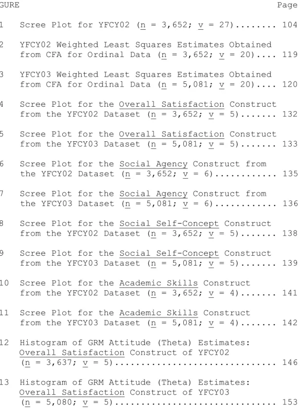
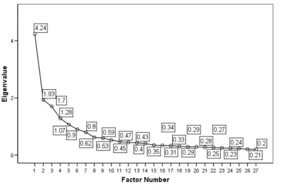
FIGURE Page 1 Scree Plot for YFCY02 (n = 3,652; v = 27)... 104 2 YFCY02 Weighted Least Squares Estimates Obtained from CFA for Ordinal Data (n = 3,652; v = 20).... 119 3 YFCY03 Weighted Least Squares Estimates Obtained from CFA for Ordinal Data (n = 5,081; v = 20).... 120 4 Scree Plot for the Overall Satisfaction Construct from the YFCY02 Dataset (n = 3,652; v = 5)... 132 5 Scree Plot for the Overall Satisfaction Construct from the YFCY03 Dataset (n = 5,081; v = 5)... 133 6 Scree Plot for the Social Agency Construct from

the YFCY02 Dataset (n = 3,652; v = 6)... 135 7 Scree Plot for the Social Agency Construct from

the YFCY03 Dataset (n = 5,081; v = 6)... 136 8 Scree Plot for the Social Self-Concept Construct from the YFCY02 Dataset (n = 3,652; v = 5)... 138 9 Scree Plot for the Social Self-Concept Construct from the YFCY03 Dataset (n = 5,081; v = 5)... 139 10 Scree Plot for the Academic Skills Construct

from the YFCY02 Dataset (n = 3,652; v = 4)... 141 11 Scree Plot for the Academic Skills Construct

from the YFCY03 Dataset (n = 5,081; v = 4)... 142 12 Histogram of GRM Attitude (Theta) Estimates:

Overall Satisfaction Construct of YFCY02

(n = 3,637; v = 5)... 146 13 Histogram of GRM Attitude (Theta) Estimates:

(10)

FIGURE Page 14 Histogram of PCM Attitude (Theta) Estimates:

(n = 3,637; v = 5)... 159 15 Histogram of PCM Attitude (Theta) Estimates:

Social Agency Construct of YFCY02

Social Self-Concept Construct of YFCY02

(11)

FIGURE Page 23 Histogram of PCM Attitude (Theta) Estimates:

Academic Skills Construct of YFCY02

(n = 5,051; v = 4)... 234 28 Scatter Plot of GRM and PCM Attitude (Theta)

Estimates: Overall Satisfaction Construct of

YFCY02 (n = 3,652; v = 5)... 248 29 Scatter Plot of GRM and PCM Attitude (Theta)

Estimates: Social Agency Construct of YFCY02

Estimates: Social Self-Concept Construct of YFCY02 (n = 3,652; v = 5)... 250 31 Scatter Plot of GRM and PCM Attitude (Theta)

Estimates: Academic Skills Construct of YFCY02

Estimates: Overall Satisfaction Construct of

(12)

FIGURE Page 33 Scatter Plot of GRM and PCM Attitude (Theta)

Estimates: Social Agency Construct of YFCY03

Estimates: Social Self-Concept Construct of YFCY03 (n = 5,082; v = 5)... 254 35 Scatter Plot of GRM and PCM Attitude (Theta)

Estimates: Academic Skills Construct of

(n = 5,082; v = 4) YFCY03... 255 36 Scatter Plot of GRM Item Discrimination Parameter (Slope) Estimates for the YFCY02 and

YFCY03 Datasets(v = 20)... 257 37 Scatter Plot of GRM and PCM Item Difficulty

Parameter (Location) Estimates for the

YFCY02 and YFCY03 Datasets (v = 20)... 258 38 Scatter Plot of GRM Item Difficulty Parameter

(Location) and Item Discrimination (Slope) Parameter Estimates for the YFCY02 and

(13)

LIST OF TABLES

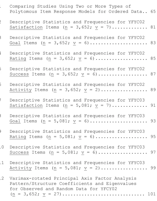
TABLE Page 1 Comparing Studies Using Two or More Types of

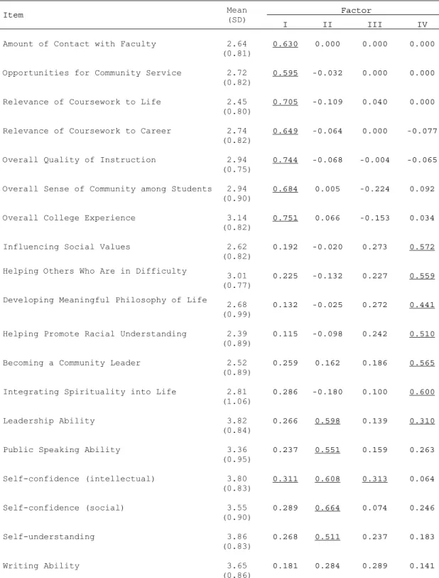
Polytomous Item Response Models for Ordered Data.. 65 2 Descriptive Statistics and Frequencies for YFYC02 Satisfaction Items (n = 3,652; v = 7)... 81 3 Descriptive Statistics and Frequencies for YFYC02 Goal Items (n = 3,652; v = 6)... 83 4 Descriptive Statistics and Frequencies for YFYC02 Rating Items (n = 3,652; v = 6)... 85 5 Descriptive Statistics and Frequencies for YFYC02 Success Items (n = 3,652; v = 6)... 87 6 Descriptive Statistics and Frequencies for YFYC02 Activity Items (n = 3,652; v = 2)... 89 7 Descriptive Statistics and Frequencies for YFYC03 Satisfaction Items (n = 5,081; v = 7)... 91 8 Descriptive Statistics and Frequencies for YFYC03 Goal Items (n = 5,081; v = 6)... 93 9 Descriptive Statistics and Frequencies for YFYC03 Rating Items (n = 5,081; v = 6)... 95 10 Descriptive Statistics and Frequencies for YFYC03 Success Items (n = 5,081; v = 6)... 97 11 Descriptive Statistics and Frequencies for YFYC03 Activity Items (n = 5,081; v = 2)... 99 12 Varimax-rotated Principal Axis Factor Analysis

Pattern/Structure Coefficients and Eigenvalues for Observed and Random Data for YFCY02

(14)

TABLE Page 13 Pattern/Structure Coefficients for the

Four-Factor Model from Ordinal Factor Analysis

for YFCY02 (n = 3,652; v = 27)... 107 14 Pattern/Structure Coefficients for the

Five-Factor Model from Ordinal Factor Analysis for YFCY02 (n = 3,652; v = 27)... 110 15 Pattern/Structure Coefficients for the

Seven-Factor Model from Ordinal Factor Analysis

for YFCY02 (n = 3,652; v = 27)... 113 16 Pattern/Structure Coefficients for the Three CFA Models for YFCY02 (n = 3,652; v = 27)... 117 17 Partial Invariance Four-Factor Model Estimates

for the YFCY02 (n = 3,652) and YFCY03

(n = 5,081) Datasets... 125 18 Full Invariance YFCY02 Data (n = 3,652) with

YFCY03 Estimates and YFCY03 Data (n = 5,081)

with YFCY02 Estimates... 128 19 GRM Item Parameter Estimates from the Main and

Subsamples of the YFCY02 Overall Satisfaction

Construct... 151 20 GRM Item Parameter Estimates from the Main and

Construct... 158 21 PCM Item Parameter Estimates from the Main and

Construct... 163 22 PCM Item Parameter Estimates from the Main and

Construct... 168 23 GRM Item Parameter Estimates for the Social

Agency Construct from the Main and Subsamples

(15)

TABLE Page 24 GRM Item Parameter Estimates for the Social

Agency Construct from the Main and Subsamples

of the YFCY03 Dataset... 179 25 PCM Item Parameter Estimates for the Social

Agency Construct from the Main and

Subsamples of the YFCY02 Dataset... 187 26 PCM Item Parameter Estimates for the Social

Agency Construct from the Main and

Subsamples of the YFCY03 Dataset... 192 27 GRM Item Parameter Estimates for the Social Self- Concept Construct from the Main and

Subsamples of the YFCY02 Dataset... 199 28 GRM Item Parameter Estimates for the Social Self- Concept Construct from the Main and

Subsamples of the YFCY03 Dataset... 202 29 PCM Item Parameter Estimates for the Social Self- Concept Construct from the Main and

Subsamples of the YFCY02 Dataset... 210 30 PCM Item Parameter Estimates for the Social Self- Concept Construct from the Main and

Subsamples of the YFCY03 Dataset... 215 31 GRM Item Parameter Estimates for the

Academic Skills Construct from the Main and

Subsamples of the YFCY02 Dataset... 221 32 GRM Item Parameter Estimates for the

Academic Skills Construct from the Main and

Subsamples of the YFCY03 Dataset... 228 33 PCM Item Parameter Estimates for the Academic

Skills Construct from the Main and Subsamples

of YFCY02 Dataset... 232 34 PCM Item Parameter Estimates for the Academic

Skills Construct from the Main and Subsamples of

(16)

TABLE Page 35 GRM and PCM Item Parameter Estimates for the

Overall Satisfaction Construct Using the YFCY02

(n = 3,652) and YFCY03 (n = 5,081) Datasets... 240 36 GRM and PCM Item Parameter Estimates for the

Social Agency Construct Using the YFCY02

Social Self-Concept Construct Using the YFCY02

Academic Skills Construct Using the YFCY02

(n = 3,652) and YFCY03 (n = 5,081) Datasets... 244 39 Eigenvalues Obtained Using Pearson Correlation

(17)

CHAPTER I

INTRODUCTION

The purpose of the present study was to examine the invariance of the factor structure and the item response model parameter estimates obtained from a set of 27 items selected from the 2002 and 2003 forms of Your First College Year (YFCY). The YFCY is administered to college freshmen at the end of their first college year. Originating in 2000, the YFCY is coordinated by the Higher Education Research Institute (HERI) in the Graduate School of

Education & Information Studies (GSE&IS) at the University of California, Los Angeles (UCLA).

The property of invariance is a fundamental concept in measurement. De Ayala (2009) explained invariance in

general terms: “We would like our measurement instrument to be independent of what it is we are measuring. If this is true, then the instrument possesses the property of

invariance” (p. 3). In practice, measurement invariance means that a test or assessment measures the same latent ______________

The style of this dissertation follows that of Educational and Psychological Measurement.

(18)

trait(s) “in the same way, when administered to two or more qualitatively distinct groups (e.g., men and women)”

(Reise, Widaman, & Pugh, 1993, p. 552). Researchers can assess measurement invariance using confirmatory factor analysis (CFA) or item response theory (IRT) models (Meade & Lautenschlager, 2004; Reise, Widaman, & Pugh, 1993).

To measure latent traits such as satisfaction with college life, YFCY items use polytomous item scales with ordered response categories (e.g., strongly disagree, disagree, agree, strongly agree). Typically, polytomous scales with ordered data are analyzed by assigning integers and then calculating and comparing means and standard

deviations. However, polytomous, ordered data (e.g., Likert scales) are problematic for traditional item

analysis (Bond & Fox, 2001) and factor analyses (Jöreskog & Moustaki, 2006).

Bond and Fox (2001) explained the primary criticism of treating ordinal data as if they were interval data:

Whenever scores are added in this manner, the ratio, or at least the interval nature for the data is being presumed. That is, the relative value of each

response category across all items is treated as being the same, and the unit increases across the rating scale are given equal value …. On the one hand, the subjectivity of attitude data is acknowledged each time the data is collected. Yet on the other hand, the data are subsequently analyzed in a rigidly

(19)

prescriptive and inappropriate statistical way (i.e., by failure to incorporate that subjectivity into the data analysis). (p. 67)

Andrich (1978a) explained, “The general approach for

overcoming objections to the integer-scoring procedure is to use a response model which keeps track of the category in which a person responds” (p. 581).

Probabilistic item response models keep track of the category in which a person responds by estimating the

probabilities of responding in each of the ways possible on a given item based on the person’s standing on an

underlying trait. For example, an individual with a high standing on a latent trait such as satisfaction with

college would be very likely to agree with an item such as “I am satisfied with my overall college experience.” The collection of probabilistic item response models comprises item response theory (IRT), also known as latent trait theory. Researcher use IRT to explore item properties and scales for tests, surveys, attitude inventories, and other assessment instruments.

IRT models require assumptions governing monotonicity, unidimensionality, and local independence of the items on a scale. Monotonicity means that the probability of passing or agreeing with an item stays the same or increases, but

(20)

never decreases, as values of the latent trait increase. In other words, the probability of agreeing with/passing an item never gets smaller as values of the latent variable increase (Millsap, 2008).

Unidimensionality means that one latent trait underlies a set of items on a test or survey.

Unidimensionality and local independence are related. Local independence means that once the appropriate number of latent traits is specified for a model, at a given value of the latent trait, item responses should be uncorrelated. Hambleton, Swaminathan, and Rogers (1991) explained: “Local independence will be obtained whenever the complete latent space has been specified: that is, when all the ability dimensions influencing performance have taken into account” (p. 11). If the assumption of unidimensionality is met, then the complete latent space is specified and there are no other relationships among the items.

In practice, researchers assess unidimensionality using exploratory factor analysis or confirmatory factor analysis (Cook, Kallen, & Amtmann, 2009). Researchers use exploratory factor analysis (EFA) when they have no ideas or theories about the number of factors underlying a latent space or the relationships among the items and factor(s).

(21)

Using confirmatory factor analysis (CFA) is appropriate when a researcher has a theory about the relationship between items and the number of factors needed to specify the latent space. For example, to test unidimensionality, a researcher could use a CFA model to evaluate how well a set of items fit a one-factor model.

The mathematical foundation of item response theory is the item response function (IRF). Item response functions are also called item characteristic curves (ICC), item

characteristic functions, and item response curves. Parametric item response models require specified

mathematical models, either a normal ogive or a logistic function, to estimate item response functions.

Item response functions provide the probabilities of responding in each category as a function of the latent trait (Ө). Thissen (2003) explained:

The attribute being measured by the test is usually called Θ and is usually arbitrarily placed on a

z-score scale, so zero is average and Θ-values range, in practice, roughly from -3 to +3. Item response theory is used to convert item responses into an estimate of

Θ, as well as to examine the properties of the items in item analysis. (p. 593)

Because of IRT’s origins in achievement and aptitude

(22)

However, in the context of attitude measurement, the latent trait is called attitude.

Modeling an item response function requires at least two parameters: a slope parameter (a) and a location

parameter (b). The slope parameter (a), also known as the scale parameter or item discrimination parameter, estimates the steepness of the item response function. The range for the slope parameter is from 0.0 to 2.0.

Higher values of the item discrimination estimate are associated with steeper slopes of the item response

functions. Baker (2001) explained that when discrimination parameter estimates are greater than 1.70 they are very high, between 1.35 and 1.70 as high, and between 0.65 and 1.34 as moderate. A steeper slope function implies that the probability of agreeing with an item increases more rapidly with increases in the latent variable (Θ) (Millsap, 2008).

The location parameter (b) indicates where the IRF is centered on the latent trait’s (Θ) continuum. The location parameter (b) is also known as the item difficulty

parameter. Ostini and Nering (2006) explained:

The center of the function is defined as midway between its lower and upper asymptotes. More

(23)

of inflection of the curve. The letter b typically signifies the item’s location parameter. (pp. 4-5) When the latent trait scale (Θ) is centered at zero, the item difficulty parameter estimates may be positive or negative, but tend to be like z-scores in range (Millsap, 2008).

Parameters for logistic item response models are

estimated using logits, or log odds-units. For dichotomous items, items with only two response categories (e.g.,

correct/incorrect, true/false, agree/disagree), a log odds is defined as the natural logarithm of the probability of success over the probability of failure.

For polytomous items, items with three or more ordered response categories (e.g., strongly disagree, disagree, agree, strongly agree), the ordered nature of the data is honored by using adjacent categories or groups of

categories. Parametric, polytomous item response models for ordered data have been classified based on how the logits are constructed (Hemker, 2001; Mellenbergh, 1995; Thissen & Steinberg, 1986). For example, a five-point scale has five response options (e.g., strongly disagree, disagree, neutral, agree, and strongly agree) and four intervals between the response options. If someone

(24)

responds Agree, there is one interval to the right and there are three intervals to the left of Agree.

Cumulative probability models (Mellenbergh, 1995) estimate the probabilities for all of the intervals to the left of the selected boundary and then any remaining

intervals to the right. Cumulative probability models are also called difference models (Thissen & Steinberg, 1986), Thurstone models (Andrich, 1995), and Thurstone/Samejima models (Ostini & Nering, 2006). Samejima’s (1969)

homogenous graded response model (GRM) is a cumulative probability model.

Adjacent category models (Mellenbergh, 1995) estimate the probabilities only for the intervals immediately to the left and the right of the selected boundary. Less

intuitive names for adjacent category models include: divide-by-total models (Thissen & Steinberg, 1986), Rasch models (Andrich, 1995), and partial credit models (Masters, 1982). Masters’ (1982) partial credit model is an adjacent category model.

While there are structural differences between cumulative probability models (difference models;

Thurstone/Samejima models) and adjacent category models (divide-by-total models; Rasch measurement models), the

(25)

models are algebraically equivalent. Thissen and Steinberg (1986) explained:

‘Difference’ models may be algebraically rearranged into ‘divide-by-total’ form… All multiple category models have both ‘difference’ and ‘divide-by-total’ forms. The models usually have relatively simple algebraic expression in their derivational form, and complex expressions in the alternative. (p. 574) Furthermore, Ostini and Nering (2006) stated, “there is little demonstrated evidence that different polytomous IRT models do produce substantially different measurement

outcomes when applied to the same data” (p. 90).

However, comparing polytomous item response model outcomes has been problematic. Ostini’s 2001 dissertation was a rigorous study “to determine what measurement

implications accompany different choices of model” (p. 31). Ostini (2001) focused specifically on the differences

between cumulative and adjacent category models. One of Ostini’s conclusions was that model fit procedures and parameter estimation methods complicated comparing results across models.

Maximum likelihood estimation (MLE) and maximum a posteriori (MAP) estimation are statistical estimation procedures for obtaining estimates for the latent trait, also known as Θ or person parameters. Ostini explained,

(26)

“It is disconcerting that a program’s default setting (e.g., MLE or MAP) could have greater influence on Θ

distribution characteristics than choice of model appeared to have” (p. 290). Ostini (2001) recommended systematic investigation of the influence of parameter estimation procedures on both person and item parameters.

Embretson and Reise (2000) provided a cautionary note regarding parameter estimation routines and IRT software:

Although many programs use a marginal maximum

likelihood procedure to estimate item parameters, a default run of the same data set through the various programs will generally not produce the exact same results. … This is important to be aware of, and researchers should not assume the IRT parameters output from these programs are like OLS [ordinary least squares] regression coefficients, where all software programs yield exactly the same results with the same data set. (p. 344)

Comparing measurement outcomes of item response models requires attention to technical details such as default software settings and parameter estimation procedures.

In addition to the difficulties with comparing item response model results across different software packages, model fit statistics complicate comparing the outcomes of item response models. Ostini (2001) explained:

The current fit results undermine the search for an answer to the question of which model is best to use for a given set of data. It does not appear that

(27)

current fit tests can provide solid guidance in this matter. (p. 301)

Evaluating item response model fit requires a “variety of procedures to be implemented, and ultimately, a scientist must use his or her best judgment” (Embretson & Reise,

2000, p. 233). Hambleton and Swaminthan (1985) recommended using three types of evidence to evaluate model fit:

Validity of model assumptions; invariance of item and ability parameters; and accuracy of model estimates.

Theoretically, when an item response model fits the data, two desirable model features are obtained: (a) item parameters are independent of the abilities of respondents; and (b) ability parameters are independent of the set of test items administered (Hambleton, Swaminathan, & Rogers, 1991). Thus, some refer to IRT person estimates as being “item free,” and item calibrations as being “person free.” These two features are called item parameter invariance and ability parameter invariance, respectively. Parameter

invariance was a major reason researchers selected item response models (e.g., Reise, Ainsworth, & Haviland, 2005; Embretson & Reise, 2000).

(28)

Statement of the Problem

In practice, measurement invariance is assessed using factor analysis methods and IRT models (Meade &

Lautenshlager, 2004). However, polytomous, ordered data are problematic for traditional item analysis (Bond & Fox, 2001) and factor analyses (Jöreskog & Moustaki, 2006).

Purpose of the Study

The purpose of the present study was to examine the invariance of the factor structure and the item response model parameter estimates obtained from two different datasets (i.e., identical items, different people).

Research Questions

The following research questions were addressed in the present study:

1. How similar/invariant are the factor structures obtained from two different datasets (i.e., identical items, different people)?

2. How similar/invariant are person and item parameter estimates obtained from two different datasets (i.e.,

identical items, different people) for the homogenous graded response model (Samejima, 1969) and the partial credit model (Masters, 1982)?

(29)

Delimitation

The models included in the present study were

restricted to parametric, unidimensional, item response models for ordered data.

Contents of the Present Study

The present study consists of five chapters. Chapter I introduces the basics of factor analysis and item

response models, the purpose of the present study, and the research questions. Chapter II provides a review of

origins and development of factor analysis and selected polytomous item response models for ordered data;

procedures for evaluating model assumptions; and procedures for evaluating model fit. Chapter III is the methods

section and explains the present study’s data analysis and software procedures. Chapter IV presents the results of the data analysis organized by research question. Chapter V is a discussion of the results, the research questions, and implications for future research.

(30)

CHAPTER II LITERATURE REVIEW

Chapter II provides a review of fundamental concepts of measurement invariance, unidimensionality, factor

analysis, and Item Response Theory (IRT). Furthermore, literature comparing polytomous item response models for ordered data was reviewed.

Measurement Invariance

The property of invariance is a fundamental concept in measurement. De Ayala (2009) explained invariance in

general terms: “We would like our measurement instrument to be independent of what it is we are measuring. If this is true, then the instrument possesses the property of

invariance” (p. 3). In practice, measurement invariance means that a test or assessment measures the same latent trait(s) “in the same way, when administered to two or more qualitatively distinct groups (e.g., men and women)”

(Reise, Widaman, & Pugh, 1993, p. 552). Researchers can assess measurement invariance using confirmatory factor analysis (CFA) or item response theory (IRT) models (Meade & Lautenschlager, 2004; Reise, Widaman, & Pugh, 1993).

(31)

Jöreskog and Moustaki (2006) explained the basic concept of factor analysis:

For a given set of manifest variables … one wants to find a set of latent variables…, fewer in number than the manifest variables, that contain essentially the same information. The latent variables are supposed to account for the dependencies among the manifest variables in the sense that if the latent variables are held fixed, the manifest variables would be independent. (p. 1)

If a researcher has no idea or theory to determine the set of latent variables, exploratory factor analysis (EFA) is appropriate. When a researcher has a theory or a specific idea about the number of factors needed to specify the latent space, confirmatory factor analysis (CFA) is appropriate.

Factor analyses methods require a series of decisions. For example, EFA requires the researcher to determine the number of factors to retain and make decisions about factor extraction and rotation method. CFA requires the

researcher to make decisions about parameter estimation routines. Gorsuch (1983) summarized when analytic

decisions may affect factorial invariance:

In factor analysis, one has numerous possibilities for capitalizing on chance. Most extraction procedures, including principal factor solutions, reach their

criterion by such capitalization. The same is true of rotational procedures, including those that rotate for simple structure. Therefore, the solutions are biased

(32)

in the direction of the criterion used. … The effects of capitalization upon chance in the interpretation can be reduced if a suggestion by Harris and Harris (1971) is followed: Factor the data by several

different analytical procedures and hold sacred only those factors that appear across all the procedures used. (p. 330)

Using multiple procedures to evaluate factor analyses results is good practice.

Mathematically, CFA models the observed response as “a linear combination of a latent variable, an item intercept, a factor loading, and some residual/error score for the item” (Meade & Lautenschlager, 2004, p. 362). In other words, CFA models the covariance between items (Reise, Widaman, & Pugh, 1993). CFA is appropriate for assessing measurement invariance because researchers can constrain the pattern/structure coefficients, error scores, and other parameter estimates to evaluate different levels of

measurement invariance (Thompson, 2004).

In the context of CFA, the least restrictive level of measurement invariance is when the CFA model fits the

datasets without any conditions imposed on the parameter estimates (Thompson, 2004). Partial measurement invariance is obtained when some of the parameter estimates are the same across datasets (Reise, Widaman, & Pugh, 1993). Full measurement invariance means that all of the parameter

(33)

estimates are the same across datasets (Reise et al., 1993).

In practice, using CFA to assess measurement

invariance entails several considerations. The first step is to run a baseline model that requires the items to load on the same factors but does not restrict parameter

estimates. Then, the fit of the baseline model needs to be examined using fit indices. If the baseline model

satisfactorily fits the data, the researcher can proceed to evaluate whether the partial and full measurement

invariance models fit the data.

To evaluate the fit of CFA models, Thompson (2004) recommended using several fit indices. Specifically, for satisfactory model fit the normed fit index (NFI) and the comparative fit index (CFI) should be greater than 0.95, and the root-mean-square error of approximation (RMSEA) should be less than 0.06 (Thompson, 2004).

Using IRT methods for evaluating measurement

invariance entails examining item discrimination (a) and item difficulty parameters (b) (Reise, Widaman, & Pugh, 1993). For polytomous data, Samejima’s homogenous graded response model (GRM; Samejima, 1969) can be used to assess measurement invariance. Meade and Lautenschlager (2004)

(34)

explained that item discrimination parameters obtained from the GRM “are conceptually analogous, and mathematically related, to factor loadings [pattern/structure

coefficients] in CFA methodology (McDonald, 1999)” (p. 366). Essentially, to evaluate measurement invariance using IRT methods, item discrimination and item difficulty parameters need to be equivalent across datasets.

Furthermore, using IRT methods to assess measurement invariance usually requires evaluating dimensionality of latent traits. Specifically, the GRM and most commonly used IRT models assume unidimensionality. Millsap (2007) explained:

Nothing in the definition of MI [measurement

invariance] requires the intended latent variable to be unitary, with only one intended latent dimension. … It is true that some latent variable models used to investigate violations of MI routinely assume

unidimensionality, examples being models based on unidimensional item response theory (IRT). (p. 462-463)

Researchers routinely use exploratory factor analysis (EFA) and confirmatory factor analysis to assess the

unidimensionality assumption of IRT models.

To determine if a set of items are unidimensional, Lord (1980) provided a “rough procedure” (p. 21). Lord advised using latent roots (eigenvalues). If the first

(35)

eigenvalue is much greater than the second and the second value is similar to the remaining eigenvalues, then “the items are “approximately unidimensional” (Lord, 1980, p. 21). Lord’s procedure for using eigenvalues to evaluate the unidimensionality assumption is used frequently in IRT literature (Dodd, 1984). To assess unidimensionality, Ostini (2001) selected parallel analysis to determine the number of factors to retain and principal axis factor analysis for extraction with VARIMAX rotation.

While using classical factor analyses methods (EFA and CFA) are popular for assessing unidimensionality of IRT models, factor analyses methods assume that the observed data and latent variables are continuous. Embretson and Reise (2000) explained that violations of the assumptions of continuous data “can and do lead to underestimates of factor loadings [pattern/structure coefficients] and/or

overestimates of the number of latent dimensions” (p. 308). Classical factor analyses use correlation or covariance

matrices of the observed variables. Using factor analysis methods intended for continuous data with ordinal data may provide misleading results.

(36)

Jöreskog (2005) objected to treating ordinal variables as if they are continuous variables:

Ordinal variables are not continuous variables and should not be treated as if they are. It is common practice to treat scores 1, 2, and 3, assigned to categories as if they have metric properties but this is wrong. Ordinal variables do not have origins or units of measurements. Means, variances, and

covariances of ordinal variables have no meaning. (p. 1)

To overcome the objection to treating ordinal data as

continuous data, Jöreskog and Moustaki (2006) advised using full information maximum likelihood estimation methods.

Thompson (2004) explained that the continuous versus ordinal data controversy depends to some extent on the judgment of the researcher. Furthermore, Thompson (2004) recommended:

Whenever there is some doubt regarding the scaling of data, or regarding the selection of matrix of

associations to analyze, it is thoughtful practice to use several reasonable choices reflecting different premises. When factors are invariant across analytic decisions, the researcher can vest greater confidence in a view that results are not methodological

artifacts. (p. 121)

Using multiple approaches to assess factor structure and unidimensionality is good practice.

In summary, CFA and IRT approaches have been used to assess measurement invariance (Millsap., 2007; Meade & Lautenschlager, 2004; Reise, Widaman, & Pugh, 1993). In

(37)

CFA, full measurement invariance is obtained when the

pattern/structure coefficients are equal (Reise, Widaman, & Pugh, 1993). If full measurement invariance is rejected, partial measurement invariance can be assessed. Partial measurement invariance is when some of the non-fixed

pattern/structure coefficients are equivalent. CFA methods are desirable for exploring relationships among latent

constructs (Meade & Lautenschlager, 2004).

To evaluate measurement invariance using IRT methods, item discrimination and item difficulty parameters need to be equivalent across datasets. Furthermore, if a

unidimensional IRT model is used to evaluate measurement invariance, a test of dimensionality is required. IRT methods are preferred when the equivalence of one scale or specific scale items are of interest, because the

discrimination (a) and item difficulty parameters (b)

“provide considerably more psychometric information at the item response level than do their CFA counterparts (item intercepts)” (Meade & Lautenschlager, 2004, p. 383).

When comparing IRT and CFA methods for evaluating measurement invariance, Meade and Lautenschlager (2004) recommended:

(38)

Under ideal conditions, it would be desirable to consider both approaches when examining ME/I [measurement equivalence/invariance]. First,

measurement equivalence could be examined using IRT methods at the item level within each scale or

subscale desired. Items that satisfy these conditions could then be used in CFA tests for individual scales and in more complex measurement models involving

several scales simultaneously. (p. 383)

Using both IRT and CFA approaches to evaluate measurement invariance provides information about the latent constructs and item level information.

Fundamental Concepts of IRT

The origins of attitude measurement involved multiple raters sorting slips of paper into categories (Allport & Hartman, 1924; Thurstone, 1928). Thurstone (1928)

presented a method for measuring attitudes using a “more” and “less” comparison providing a linear scale for attitude measurement. Thurstone’s (1928) method entailed measuring an individual’s attitude “as expressed by the acceptance or rejection of opinions” (p. 533). Thurstone (1928)

explained:

The main argument so far has been to show that since in ordinary conversation we readily and understandably describe individuals as more and less pacifistic or more and less militaristic in attitude, we may frankly represent this linearity in the form of a

(39)

Thurstone’s method for attitude scaling assumed the attitude being measured was normally distributed in the population and the set of items were unidimensional.

Likert (1932) acknowledged Thurstone’s procedures were “characterized by a special endeavor to equalize the step-intervals from one attitude to the next in the attitude scale” (p. 5). Likert (1932) asked two compelling

questions about Thurstone’s method of attitude measurement: The method is exceedingly laborious. It seems

legitimate to inquire whether it actually does its work better than simpler scales which may be employed, and in the same breath to ask also whether it is not possible to construct equally reliable scales without making unnecessary statistical assumptions. (p. 6) Likert’s primary criticism of Thurstone’s method involved the statistical assumption that attitudes were normally distributed.

Likert’s (1932) method for scoring attitudes assumed “a linear relationship between the response probability and the underlying trait” (Ostini & Nering, 2006, p. 7) and the assumption that attitudes are distributed normally in the population. Likert (1932) explained:

Assuming that attitudes are distributed normally, a method of measuring attitudes has been developed which uses sigma units. This method not only retains most of the advantages present in methods now used, such as yielding scores the units of which are equal

(40)

advantages. These briefly are: first, the method does away with the use of raters or judges and the errors arising therefrom; second, it is less laborious to construct an attitude scale by this method; and third, the method yields the same reliability with fewer

items. (p. 42)

Likert (1932) concluded that his sigma method was not an improvement on assigning consecutive integers to response categories and obtaining a score for each person “by

finding the average or sum of the numerical values of the alternatives that he checked” (p. 42). Likert’s conclusion about averaging integers assigned to response categories generated 70 years of enduring controversy.

Bond and Fox (2001) explained the primary criticism of treating ordinal data as if they were interval data:

Whenever scores are added in this manner, the ratio, Or at least the interval nature for the data is being presumed. That is, the relative value of each

response vategory across all items is treated as being the same, and the unit increases across the rating scale are given equal value…. On the one hand, the subjectivity of attitude data is acknowledged each time the data is collected. Yet on the other hand, the data are subsequently analyzed in a rigidly

prescriptive and inappropriate statistical way (i.e., by failure to incorporate that subjectivity into the data analysis). (p. 67)

Andrich (1978a) explained, “The general approach for

overcoming objections to the integer-scoring procedure is to use a response model which keeps track of the category in which a person responds” (p. 581). Probabilistic item

(41)

response models keep track of the category in which a person responds by estimating the probabilities of

responding in each of the ways possible on a given item based on the person’s standing on an underlying trait.

Originally, the family of item response models was called latent trait theory, also known as item response theory (IRT). Moustaki (2007) explained that latent trait models mean that the latent/underlying variable, the

dependent variable, is a continuous and the manifest variables are categorical. In contrast, factor analyses models have continuous latent variables and continuous manifest variables (Moustaki, 2007). Item response models estimate the probability of a person responding in each of the ways possible on a given item based on the person’s standing on an underlying trait.

Polytomous item response models for ordered data developed in two major branches: Rasch measurement models (Masters, 1982; Rasch, 1960/1980; Rost, 1988); and,

Thurstone/Samejima models (Bock, 1972; Muraki, 1992; Samejima, 1969). Both the Rasch and Thurstone/Samejima proponents credit Thurstone with the origins of

(42)

While addressing concerns about validity of measures, Thurstone (1928) stated:

A measuring instrument must not be seriously affected in its measuring function by the object of

measurement. To the extent that its measuring function is so affected, the validity of the

instrument is impaired or limited. If a yardstick measured differently because of the fact that it was a rug, a picture, or a piece of paper that was being measured, then to the extent the trustworthiness of that yardstick as a measuring device would be

impaired. Within the range of objects for which the measuring instrument is intended, it function must be independent of the object of measurement. (p. 547) The Rasch and IRT camps invoked the phrases “objective measurement” and “objective measure,” respectively,

(Samejima, 1972; Wright & Stone, 1979) when advocating the benefits of probabilistic item response models yielding person-free and item-free statistics.

Adjacent Category Models

Item response functions model two distinct conditional probabilities: item category response functions (ICRFs) and category boundary response functions (CBRFs). The item category response function (ICRF) models the probability of an individual responding a given way in a specific

category. The category boundary response function (CBRF) estimates the probability of an individual “responding

(43)

positively rather than negatively at a given boundary between two categories” (Ostini & Nering, 2006, p. 9).

For dichotomous items, items with only two response categories (e.g., correct/incorrect, true/false,

agree/disagree), the item category response function and the category response function are equivalent. Ostini and Nering (2006) explained that “the probability of responding positively rather than negatively at the category boundary … also represents the probability of responding in the positive category” (p. 9).

However, for polytomous items “the probability of responding positively rather than negatively at a given boundary between two categories” has at least two

interpretations. Ostini and Nering (2006) explained:

‘Positively rather than negatively’ can refer to just the two categories immediately adjacent to the

category boundary …. Alternatively, the phrase can refer to all of the possible response categories for an item above and below the category boundary

respectively. (p. 13)

Adjacent category models (Mellenbergh, 1995) use only the two categories immediately adjacent to the selected

category boundary to obtain CBRFs. Cumulative probability models (Mellenbergh, 1995) obtain CBRFs by using all of the

(44)

possible response categories to the left and to the right of the selected category boundary.

Less intuitive names for adjacent category models include: divide-by-total models (Thissen & Steinberg, 1986), Rasch models (Andrich, 1995), and partial credit models (Masters, 1982). Andrich’s (1978a) rating scale model (RSM) is an adjacent category model requiring the following assumptions: All items in the item set have the same scale and format and all items have equal item

discrimination parameter estimates. The partial credit model (Masters, 1982) can be used when the number of response categories is different among a set of items.

Rasch Measurement Models

Rasch (1960/1980) addressed item and test properties using probability theory and “ignored the existing

literature on both IRT and classical test theory” (Baker & Kim, 2004, p. 154). In the context of attitude

measurement, Andrich (1978b) explained Rasch measurement “provides a perspective for unifying the Thurstone goal of item scaling and the Likert procedure for attitude

measurement” (p. 667). Andrich (1978b) and Wright and Masters (1982) extended the work of Rasch (1960/1980) to

(45)

develop the rating scale and partial credit models, respectively.

Embretson and Reise (2000) provided a cautionary note about the literature on rating scale models: “The

literature on the ‘rating scale model’ can be a little confusing because there are several versions of this model that vary in complexity and are formulated in different ways by different authors” (p. 115). Andrich (2005) explained “that the so called rating scale and partial

credit models, at the level of one person responding to one item, are identical in their structure and in the response process they can characterise [sic]” (p. 31). The

fundamental assumption of Andrich’s (1978a) rating scale model assumes that all of the items on a scale have the same discrimination (slope) parameter.

The partial credit model (Masters, 1982) is an

extension of Andrich’s rating scale model that preserves the desirable features of Rasch models. Masters explained:

The parameters in this ‘Partial Credit’ model appear additively in the exponent of the model and so can be separated and estimated independently of each other. This separability results in sufficient statistics for the model parameters and makes possible objective

comparisons of persons and items from graded responses. (p. 149)

(46)

The primary distinction between the rating scale model and the partial credit model is that the partial credit model can be used when the number of response categories is different among a set of items.

The mathematical statement of the partial credit model is the probability of an individual responding in a

specific category is a function of the difference between the individual’s trait level and a category intersection parameter (Embretson & Reise, 2001). The mathematical expression of Master’s (1982) partial credit model (PCM) for the present study is:

exp[a ∑(Ө - bik)] k=0 Pij(Ө) = ____________________ , mj-1 j ∑ [exp a ∑(Ө - bik)] j=0 k=0

Where Pij(Ө) is the probability of selecting category j in

item i, at a given Ө. The item discrimination parameter, a, is constant across items, and the bij term is the item

step difficulty for category j. The greater the value of the item step difficulty, the more “difficult” (i.e., less likely) the specific step is compared to other steps in the item.

Separability. Rasch models have a property called

(47)

Mathematically, item difficulty parameters are estimated without estimating respondents’ attitudes. Masters (1982) provided an accessible explanation of the property of

separability:

In common with all Rasch models, the parameters … appear additively in the exponent of the model and so can be separated and estimated independently of each other. This separability results in sufficient

statistics for the model parameters and makes possible objective comparisons of persons and items from graded responses. (p. 149)

In practice, the property of separability means that if a Rasch model fits the data, then the sum score is a

sufficient statistic and can be used to obtain parameter estimates.

Rost (2001) explained how the property of separability influences the item characteristic curves (ICCs):

Separability denotes the property that person and item effects on the response behavior can be isolated from each other. This can be seen as an analogy to

analysis of variance where the separation of two

factors in a main effects model implies that there are no interaction effects between these factors. It

follows from this analogy that intersecting ICCs would contradict separability, since it is kind of

interaction: intersecting ICCs means that the ‘effect size’ of the person factor with respect to the

response probability varies from item to item. (p. 28).

Separable person and item parameters allow “person parameters to be conditioned out of item calibration,

(48)

enabling sample-free calibration, and item parameters to be conditioned out of person measurements, enabling test-free measurement” (Wright & Masters, 1982, p. 59).

Andrich (1978b) explained the practical implications of separability and sufficient statistics when a Rasch model fits the data:

Consequently, if the model holds, the pattern of

responses of subjects or items is immaterial for their respective parameter estimates. Their respective

total scores are sufficient. It is of particular interest that in the first stage in estimating a

person’s attitude, his scores on the items are simply summed as in the Likert procedure with no reference to the scale values of the items. (p. 670)

If a Rasch measurement model fits the data, adding integers is an acceptable procedure for obtaining respondent scores and parameter estimates.

Cumulative Probability Models

Cumulative probability models are also called

difference models (Thissen & Steinberg, 1986), Thurstone models (Andrich, 1995), and Thurstone/Samejima models (Ostini & Nering, 2006). Samejima’s (1969) homogenous graded response model (GRM) is a cumulative probability model. Mellenbergh (1995) explained that cumulative

probability models preserve the ordinal nature of the data by using pairs of categories. Cumulative probability

(49)

models estimate the probabilities for all of the intervals to the left of the selected boundary and then any remaining intervals to the right.

Samejima Models

Samejima (1998) explained that the graded response model “represents a family of mathematical models that deals with ordered polytomous categories” (p. 85).

Samejima (1972) presented two classes of graded response models: heterogeneous and homogenous graded response

models. Samejima (1969) developed the homogeneous response model using the normal ogive and logistic function.

Samejima (1969) explained that the homogenous graded response models, logistic and normal ogive, are homogenous because “sometimes the reasoning required in solving the discriminating power should be almost constant throughout the whole thinking process required in solving the problem” (p. 19). The discrimination parameter (slope) of

homogenous graded response models must be the same for all categories within an item, but can vary across a set of items. In other words, the category boundary response functions of the homogenous graded response model can

differ across a set of items, but not within a single item (Ostini & Nering, 2006).

(50)

The mathematical statement of Samejima’s 1969 homogenous graded response model using the logistic function is:

Pig = __exp[ai(Ө - big)]__

1 + exp[ai(Ө - big)]

The ai is the item discrimination parameter and big is the

item difficulty parameter, also known as the boundary location parameter. Because the graded response model is homogenous, item discrimination is constant within the item and only one item slope parameter (a) is estimated. Each between-category threshold must be estimated by item

difficulty parameters (b). Embretson and Reise (2000)

explained that the difficulty parameters are interpreted as the value of the latent trait required to respond above each threshold with a 0.50 probability.

Ostini (2001) described Samejima’s 1969 homogenous graded response model as “the archetypal” cumulative probability model (p. 12). For cumulative probability models, the categories of the ordinal variable are split into one less cumulative probability than the number of categories. For example, four ordered categories are

divided into three conditional probabilities. Mellenbergh (1995) explained “the ordered nature of the variable is

(51)

preserved by using contiguous groups of categories” (p. 94). Cumulative probability models can be used to model items with different numbers of categories.

Parameter Estimation

The purpose of IRT is to estimate both the value of the latent trait for each respondent and the item

parameters for each item. At the beginning of an analysis, the responses to the items are known, but the item

parameters are also unknown and the respondents’ values on the latent trait are unknown. Parameter estimation uses the observed, known responses to find the item

characteristic curves that best fit the selected item response model (Baker, 2001). Thissen (2003) explained:

The power of IRT is associated primarily with the phrase ‘estimate the value of the trait’. Loosely speaking, we say that a test is ‘scored’. But

strictly speaking the test is not scored; one does not simply count the positive responses, as is done in traditional test theory. One ‘estimates the value of the trait’ using the inferred relationships between the item responses and the trait being measured. (p. 592)

Essentially, parameter estimation uses known information, individuals’ responses to a set of items, to obtain values for the unknown item parameters and latent trait values.

To obtain estimates of the person and item parameters (latent trait values/scores), the parametric item response

(52)

function requires a mathematical form such as the normal ogive or logistic functions. Baker and Kim (2004)

explained:

Switching from a normal ogive to a logistic ogive model for an item’s ICC results in a significant decrease in the computational demands of the maximum likelihood estimation procedure. Since the cumulative distribution of the logistic density has a closed

form, that is, does not involve an integral, it can be computed easily. This computational advantage is the primary reason for using logistic ogive models for the ICC. (p. 38)

Normal ogive and logistic item response models function predict nearly identical item characteristic curves with the greatest differences occurring at extreme levels of latent trait scores (Embretson & Reise, 2000).

Parameter estimation requires assumptions about local independence and unidimensionality. Lord (1980) explained:

Local independence requires that any two items be uncorrelated when Ө [theta – the underlying latent variable] is fixed. It definitely does not require that items be uncorrelated in ordinary groups, where Ө

varies. Note in particular that local independence follows automatically from unidimensionality. It is not an additional assumption. (p. 19)

Mathematically, local independence means “the probability of success on all items is equal to the product of the separate probabilities of success” (Lord, 1980, p. 19).

Embretson and Reise (2000) explained the importance of the local independence assumption in parameter estimation:

(53)

To apply an IRT model, local independence must be assumed because the response pattern probability is the simple product of the individual item

probabilities. If local independence is violated, Then the response pattern probabilities will be inappropriately reproduced in standard IRT models. (p. 188)

Local independence is required to obtain estimates of response pattern probabilities.

In practice, selecting a parameter estimation method is limited by the software package a researcher uses. For example, Parscale 4.0 for Windows (Muraki & Bock, 2008) obtains latent trait estimates using maximum likelihood estimation (MLE), weighted maximum likelihood (WML), or expected a posteriori (EAP). To obtain item parameter estimates, Parscale 4.0 uses maximum likelihood estimation (MLE) and marginal maximum likelihood estimation (MMLE).

There are two major classes of parameter estimation theories: Maximum likelihood estimation (MLE) and Bayesian methods. Wang and Vispoel (1998) explained a basic

difference between MLE and Bayesian estimation is that Bayesian methods “incorporate prior information into the data in deriving ability estimates, whereas MLE relies on the data alone” (p. 110). Weighted maximum likelihood estimation belongs to the maximum likelihood class.

(54)

Expected a posteriori and marginal maximum likelihood estimation (MMLE) are Bayesian procedures.

Maximum Likelihood Estimation (MLE)

Embretson and Reise (2000) explained that maximum likelihood estimation identifies the value of the

underlying trait “that maximizes the likelihood of an examinee’s item response pattern” (p. 159). Maximum

likelihood estimation requires that the latent trait have a normal distribution (Woods, 2007) and “that the data have at least an approximately multivariate normal distribution” (Thompson, 2004, p. 127). Samejima (1972) explained, “When the distribution of the trait is unknown, maximum

likelihood estimation will be the most reasonable method” (p. 7).

Maximum likelihood estimation is not influenced by the use of logistic or normal ogive functions. Baker and Kim (2004) explained, “Changing from the normal ogive model to the logistic ogive model for the item characteristic curve has no impact upon the framework of the maximum likelihood estimation procedures” (p. 38). The purpose of parameter estimation is to find the item characteristic curves, normal or logistic, that best fit the selected item response model.

(55)

Maximum likelihood estimation is an iterative

procedure that repeatedly “tweaks” the estimate until some criterion is sufficiently optimized. The first step uses start values to obtain likelihood estimates. Optimization methods are used to generate start values. The second step evaluates the change in the likelihood estimates. The

process is iterative because the first and second stages are repeated until there is very little change in the estimates or the estimates “converge.” Millsap (2008) explained “the process of generating well ‘guesses’ is the key to the success of the method. If guesses are ‘bad’, the iterations could keep going on indefinitely” (p. 3).

When the procedure has converged, there is no promise that the converged solution is the most optimal solution. Millsap (2008) explained: “For example, in maximizing the likelihood, the optimization may arrive at a local optimum.

To check this, one can re-start the procedure using a different initial value to see if the same converged solution appears” (p. 4). Failing to converge on a

solution indicates problems with model-data fit. Linacre (1987) explained, “A data set showing lack of convergence can usually be rescued by setting aside for separate study

(56)

the person or item performances which contain these unexpected responses” (p. 7).

Another limitation of maximum likelihood estimation is there are no meaningful maximum likelihood estimates when someone responds to all of the items on a survey or test in the same way, or if all of the respondents answer an item in the same way. While the items or individuals with uniform responses may be eliminated from the analysis, including them will not influence the estimates for the items and latent variables score (Lord, 1980).

Weighted Maximum Likelihood Estimation (WMLE)

Weighted maximum likelihood estimation is also called weighted likelihood estimation (WLE) and Warm’s weighted maximum likelihood estimation (Warm, 1989). Warm (2007) explained:

Maximum likelihood estimates are the parameter values which maximize the likelihood that the observed data would have been generated. Thus MLE values correspond to the mode of the likelihood function [and] modal estimates are biased when viewed from the likelihood function as whole. (p. 1094)

Warm (1989) recommended using the mean of the likelihood function as opposed to the mode of the likelihood function and concluded that WMLE estimates for latent variable

(57)

scores have “a small bias and are computationally efficient” (p. 428).

Expected a Posteriori (EAP)

Expected a posteriori (EAP) estimation is a Bayesian estimation method. Chen, Hou, Fitzpatrick, and Dodd (1997) explained “Bayesian estimation methods take a prior

population distribution into account as prior information and estimate trait levels based on the posterior

distribution (posteriori distribution α likelihood function x prior distribution)” (p. 423). EAP estimates are the mean of the posteriori distribution (Chen et al., 1997). Hambleton, Swaminathan and Rogers (1991) explained one advantage of Bayesian methods over MLE is that Bayesian estimates of the latent variable “can be obtained for zero items correct and perfect response patterns” (p. 39).

Marginal Maximum Likelihood Estimation (MMLE)

Marginal maximum likelihood estimation (MMLE) is a Bayesian procedure to estimate item parameters. MMLE assumes that the latent variable (Θ) is normally

distributed. Woods (2007) explained that “integration with respect to the continuous latent variable is done

numerically by representing as Θ as series of discrete quadrature points” (p. 73).