Asset Pricing Tests with Long Run Risks in Consumption Growth

(1)

NBER WORKING PAPER SERIES

ASSET PRICING TESTS WITH LONG RUN RISKS IN CONSUMPTION GROWTH George M. Constantinides

Anisha Ghosh Working Paper 14543

http://www.nber.org/papers/w14543

NATIONAL BUREAU OF ECONOMIC RESEARCH 1050 Massachusetts Avenue

Cambridge, MA 02138 December 2008

We thank Ravi Bansal, Alan Bester, John Campbell, Raj Chakrabarti, John Cochrane, Eugene Fama, Lars Hansen, Christian Julliard, Dana Kiku, Ralph Koijen, Oliver Linton, Sydney Ludvigson, Alex Michaelides, Lubos Pastor, Annette Vissing-Jorgensen, and Amir Yaron for helpful comments. We remain responsible for errors and omissions. Constantinides acknowledges financial support from the The Center for Research in Security Prices of the University of Chicago Booth School of Business. Ghosh acknowledges financial support from the London School of Economics. The views expressed herein are those of the author(s) and do not necessarily reflect the views of the National Bureau of Economic Research.

NBER working papers are circulated for discussion and comment purposes. They have not been peer-reviewed or been subject to the review by the NBER Board of Directors that accompanies official NBER publications.

(2)

Asset Pricing Tests with Long Run Risks in Consumption Growth George M. Constantinides and Anisha Ghosh

NBER Working Paper No. 14543 December 2008, Revised January 2011 JEL No. G12

ABSTRACT

A novel methodology in testing the long-run risks model of Bansal and Yaron (2004) is presented based on the observation that, under the null, the potentially latent state variables, "long-run risk" and the conditional variance of its innovation, are known a¢ ne functions of the observable market-wide price-dividend ratio and risk free rate. In linear forecasting regressions of consumption growth and returns by the price-dividend ratio and risk free rate, the model implies much higher forecastability than what is observed in the data over 1931 –2009. The co-integrated variant of the model by Bansal, Gallant, and Tauchen (2007), also implies much higher forecastability of returns than what is observed in the data. Finally, we reject the models' implications in jointly pricing the cross-section of returns and fitting the unconditional time series moments of consumption and dividend growth. The results suggest that either some important state variable is missing or that the models should be generalized in a way that the lagged price-dividend ratio and risk free enter the regressions in a non-linear fashion. George M. Constantinides

The University of Chicago Booth School of Business 5807 South Woodlawn Avenue Chicago, IL 60637

and NBER

[email protected] Anisha Ghosh

Tepper School of Business Carnegie Mellon University 5000 Forbes Avenue

Pittsburgh PA 15213 [email protected]

(3)

1 Introduction

A burgeoning literature in …nance addresses investors’ attitudes towards the timing of resolution of uncertainty of future consumption and cash ‡ows through the class of preferences introduced by Epstein and Zin (1989), Kreps and Porteus (1978), and Weil (1989). Models initiated by Bansal, Dittmar, and Lundblad (2005), Bansal and Yaron (2004), and Hansen, Heaton, and Li (2008) have rich implications on prices and show promise in explaining the time series and cross-sectional properties of returns of …nancial assets. These models pay particular attention to the low frequency properties of the time series of dividends and aggregate consumption— hence their characterization as “long run risks” (LRR) models.1

In this paper we revisit the particular LRR model introduced by Bansal and Yaron (2004) (hereafter B-Y) that has received wide attention in the literature. Whereas we formally reject both this model and its co-integrated variant introduced by Bansal, Gallant, and Tauchen (2007), our primary contribution lies in the novelty of our em-pirical methodology which provides new insights and guides our search for promising models of long run risks.

Our …rst methodological contribution addresses the feature of the B-Y model (and of related models) that the LRR variable and the conditional variance of its innovation are latent. The …ltering of these latent variables potentially introduces observation error and decreases the power of the tests. We argue that these “latent”state variables are, in fact, observable because both the aggregate price-dividend ratio and risk free rate are functions of only these two state variables under the model assumptions. Speci…cally, in the log-linearized version of the B-Y model, the aggregate log price-dividend ratio and log risk free rate are a¢ ne functions of the two state variables, with coe¢ cients that are known functions of the preference parameters and of the parameters of the time-series processes. This observation allows us to invert the a¢ ne system and express the two state variables as known a¢ ne functions of the observable aggregate log price-dividend ratio and log risk free rate. Whereas this empirical methodology is common in the context of the class of a¢ ne term structure models (for example, Dai and Singleton (2000) and Du¤ee (2002)), it has not previously been employed in testing LRR models. The second methodological contribution stems from the fact that the log-linearized version of the B-Y model implies that the expected market return, equity premium, dividend growth, and consumption growth are a¢ ne functions of the two state vari-ables. Since the state variables themselves are known a¢ ne functions of the observable 1_{See also, Alvarez and Jerman (2005), Bansal, Dittmar, and Kiku (2009), Bansal, Gallant, and} Tauchen (2007), Bansal, Kiku, and Yaron (2007), Bansal and Shaliastovich (2010), Beeler and Camp-bell (2009), Bekaert, Engstrom, and Xing (2009), Chen, Favilukis, and Ludvigson (2008), Colacito and Croce (2005), Constantinides and Ghosh (2010), Croce, Lettau, and Ludvigson (2008), Ferson, Nallareddy, and Xie, (2009), Ghosh and Constantinides (2010), Hansen and Scheinkman (2009), Let-tau and Ludvigson (2009), Lustig, Van Nieuwerburgh, and Verdelhan (2008), Malloy, Moskowitz, and Vissing-Jorgensen (2008), Parker and Julliard (2005), and Piazzesi and Schneider (2006).

(4)

aggregate log price-dividend ratio and log risk free rate, it follows that the expected market return, equity premium, dividend growth, and consumption growth are a¢ ne functions of the observable aggregate log price-dividend ratio and log risk free rate. Therefore, the time-series properties of the model are readily testable with in-sample linear forecasting regressions and out-of-sample linear predictive regressions of the mar-ket return, equity premium, dividend growth, and consumption growth on the lagged price-dividend ratio and risk free rate. The tests on the predictability of the market return, equity premium, and dividend growth are robust to observation error of con-sumption ‡ows and the possibility of improper temporal aggregation of concon-sumption ‡ows because consumption data are not used in these tests.

Our third methodological contribution is based on the fact that the log-linearized version of the B-Y model implies that the log pricing kernel is an a¢ ne function of the two state variables and their lags. Since the state variables themselves are known a¢ ne functions of the observable aggregate log price-dividend ratio and log risk free rate, it follows that the log pricing kernel is an a¢ ne function of the aggregate log price-dividend ratio, the log risk free rate, and their lags, in addition to consumption growth. Thus we obtain a set of Euler equations of consumption for the cross-section of returns.

The …nal methodological contribution lies in simultaneously testing through GMM the Euler equations of consumptionand the restrictions imposed on the model parame-ters by the unconditional moments of the aggregate dividend and consumption growth, thereby increasing the power of the test.

Our …rst set of tests is motivated by the implications of the B-Y model regard-ing in-sample forecastregard-ing and out-of-sample prediction of the market return, equity premium, dividend growth, and consumption growth through linear regressions on the lagged price-dividend ratio and risk free rate.2 _{Speci…cally, we simulate the B-Y model,}

calibrated at the monthly, quarterly, and annual frequencies, and demonstrate that the model implies much higher predictability of the aggregate consumption growth rate, market return, and equity premium than that observed in the data over1931_¬2009. The out-of-sample predictability tests produce negative results as well. Furthermore, the model calibrated at the annual frequency implies much higher predictability of the3-year and 5-year consumption growth rate compared to the historical data. The co-integrated variant of the model by Bansal, Gallant, and Tauchen (2007), that intro-duces as an additional state variable the consumption-dividend ratio, when calibrated at the annual frequency implies forecastability of consumption and dividend growth 2_{The predictability of the market return, equity premium, dividend growth, and consumption} growth through linear regressions on the lagged price-dividend ratio and risk free rate has been the subject of an extensive literature. Examples include Ang and Bekaert (2007), Binsbergen and Koijen (2010), Boudoukh, Richardson, and Whitelaw (2008), Campbell and Shiller (1988), Campbell and Thompson (2008), Cochrane (2008), Fama and French (1988), Kelly and Pruitt (2010), Lettau and Van Nieuwerburgh (2008), and Welch and Goyal (2008)).

(5)

consistent with the historical data. However, it implies much higher forecastability of the market return and premium than that observed in the data. Moreover, like the B-Y model, the cointegrated model performs poorly in predicting out-of-sample the growth rates and returns. Overall, these results provide robust time series evidence against the LRR model of B-Y and its co-integrated variant and suggest that either some impor-tant state variable is missing or that the model should be generalized in a way that the lagged price-dividend ratio and risk free enter the regressions in a non-linear fashion.

In simultaneously testing through GMM the Euler equations of consumption for the market return and risk free rate and the restrictions imposed on the model parameters by the unconditional moments of the aggregate dividend and consumption growth over

1931_¬ 2009, we …nd that the pricing error for the risk free rate is 33% and that for the market return is 19%. When we extend the asset system to include the "Value", "Growth", "Small" capitalization, and "Large" capitalization portfolios in addition to the market return and risk free rate, we …nd that the "Small" capitalization portfolio has pricing error 26% and the "Growth" portfolio has pricing error ¬29%. The co-integrated variant of the model by Bansal, Gallant, and Tauchen (2007) produces similar results. The overidentifying restrictions test has p-value smaller than 1% for each model speci…cation.

We address the potential problem of temporal aggregation of consumption by re-peating our estimation and tests using quarterly data over the post-war period. The results are very similar to those obtained using annual data over the sub-period, sug-gesting that our …ndings are unlikely to be driven by problems associated with temporal aggregation.

The paper is organized as follows. In Section 2, we describe the estimation and testing methodology of the LRR model. We discuss the data in Section 3. In Section

4, we present the results of the in-sample forecasting regressions and the out-of-sample predictive regressions. In Section 5, we present the empirical evidence on the cross-section of returns. In Section 6, we consider an extension of the LRR model that introduces, as a third state variable, the co-integrating residual of the logarithms of consumption and aggregate dividend levels. In Section7, we address the possibility of structural breaks within the period1931¬2009 by repeating our tests in the post-war sub-period. We also address the issues related to temporal aggregation of consumption by repeating our tests with quarterly data. Section8concludes. The appendix contains derivations and details of the testing methodology.

2 The Model and Its Testable Implications

We describe the LRR model of B-Y and derive its testable implications for the pre-dictability of the market return, equity premium, dividend growth, and consumption growth. Then we derive its testable implications for the equity premium and the

(6)

cross-section of returns.

2.1 Model

The Bansal and Yaron (2004) LRR model introduces the novel state variable, ,

and the variance of its innovation, 2_, that jointly drive the conditional mean of the aggregate consumption and dividend growth rates:

+1 = +  +1, (1)

2

+1 = (1¬ ) 2+ 2 +  +1, (2)

+1 =  ++ +1, (3)

+1 = + x+' +1, (4)

where+1 is the logarithm of the aggregate consumption level and+1 is the logarithm

of the aggregate stock market dividends. The shocks+1,  +1,+1, and+1 are

assumed to be  (01) and mutually independent. The time-series speci…cation in equations (1)-(4) introduces nine parameters: _, _, , , _, _, , , and . In

Appendix1, we derive various unconditional moments of consumption and dividend growth rates as functions of the time-series parameters.

The model further assumes that the consumer has the version of Kreps and Porteus (1978) preferences adopted by Epstein and Zin (1989) and Weil (1989). These prefer-ences allow for separation between the coe¢ cient of risk aversion and the elasticity of intertemporal substitution. The utility function is de…ned recursively as

 = h (1_¬ ) 1¬  + ¬  1+1¬ 1i₁_¬ , (5)

where denotes the subjective discount factor, 0is the coe¢ cient of risk aversion,  0 is the elasticity of intertemporal substitution, and = ₁1¬

¬1 . Note that the sign of depends on the relative magnitudes of and . The standard time-separable power utility model is obtained as a special case when = 1, i.e. = 1_.

For this speci…cation of preferences, Epstein and Zin (1989) and Weil (1989) show that, for any asset, the …rst-order conditions of the consumer’s utility maximization yield the Euler equation,

[exp(+1++1)] = 1, (6)

where

(7)

is the natural logarithm of the intertemporal marginal rate of substitution;[]denotes

expectation conditional on time  information; +1 is the continuously compounded

return on asset j; and +1 is the unobservable continuously compounded return on

an asset that delivers aggregate consumption as its dividend each period.

We rely on log-linear approximations for the log return on the consumption claim, +1, and on the market portfolio (the return on the aggregate dividend claim),+1,

as in Campbell and Shiller (1988):

+1 = 0+ 1+1¬+ +1, (8)

+1 = 0+ 1+1¬+ +1, (9)

where  is the log price-consumption ratio and  the log price-dividend ratio. In

equation (8), 1 = 



1+ and 0 = (1 +)¬ 1 are log-linearization constants, where  denotes the long-run mean of the log price-consumption ratio. Similarly, in equation (9), 1 = 



1+ and 0 = (1 +)¬ 1, where  denotes the

long-run mean of the log price-dividend ratio.

B-Y show that  and , are a¢ ne functions of the state variables, and 2,

 = 0+1+2 2, (10)

 = 0+1+2 2. (11)

The coe¢ cients 0, 1, 2, 0, 1, and 2 depend on the parameters of the

utility function and those of the stochastic processes for consumption and dividend growth rates (see Appendix A.2.1 for expressions for these coe¢ cients).

For this model speci…cation, the log risk free rate from period to+ 1may also be expressed as an a¢ ne function of the state variables (see Appendix A.2.2 for expressions for 0, 1, and 2),

 = ¬log[exp(+1)],

= 0 +1+2 2. (12)

Equations (11) and (12) express the observable variables,  and , as a¢ ne

functions of the latent state variables,  and 2. These equations may be inverted to

express the unobservable state variables,  and 2, as a¢ ne functions of the

observ-ables,  and , (see Appendix A.2.3 for details and expressions for 0, 1, 2, 0, 1, and 2),

 = 0+ 1+ 2, (13)

2

(8)

2.2 Testable Implications for Predicting Returns and Growth

Rates

Equations (9), (11), (4) and (12) imply that the expected market return is given by

[+1] =0+1+2 2, (15)

and the expected equity premium is given by

[+1¬] =0+1+2 2, (16)

both a¢ ne functions of the state variables,  and 2. The model generates

time-varying expected market return and premium. The coe¢ cients _f g2=0 are known

functions of the underlying time-series and preference parameters.

The time series speci…cation of the model implies that the expected consumption growth rate is given by

[ +1] = +, (17)

and the expected dividend growth rate is given by

[ +1] = + x, (18)

both a¢ ne functions of the state variable .

Since the state variables,  and 2 are a¢ ne functions of the observables and

, we may express the expected market return, equity premium, dividend growth, and

consumption growth as a¢ ne functions of the observables and with coe¢ cients

known functions of the model parameters.

In Section 4, we test the predictive implications of the model through in-sample lin-ear forecasting regressions and out-of-sample linlin-ear predictive regressions of the market return, equity premium, dividend growth, and consumption growth on the lagged price-dividend ratio and risk free rate.

2.3 Testable Implications for the Equity Premium and the

Cross-Section of Returns

We substitute the log-a¢ ne approximation for+1 in equation (8) into the expression

for the pricing kernel (equation (7)), and noting that  is given by equation (10), we

have,

+1 = ( log + ( ¬1) [ 0+ ( 1¬1)0]) + ¬ + ( ¬1) +1

(9)

Equation (19) for the pricing kernel involves the unobservable (from the point of view of the econometrician) state variables,  and 2, and, hence, is not directly

testable on a cross-section of asset returns. Substituting the expressions for  and 2

from equations (13) and (14) into the pricing kernel in equation (19), we have,

+1 =1 +2 +1+3 +1¬ 1 1  +4 +1¬ 1 1  . (20)

The parameters  = (1 2 3 4)0 are functions of the parameters of the time-series

processes and the preference parameters (see Appendix 24 for details). The above expression for the pricing kernel is entirely in terms of observables. We substitute this expression into the set of Euler equations (6) to obtain a set of moment restrictions that are expressed entirely in terms of observables.

We …rst examine the empirical plausibility of the model when the set of assets consists of the market portfolio and the risk free rate, thereby focusing on the equity premium and risk free rate puzzles. To the set of their Euler equations we add moment restrictions implied by the time-series speci…cation of the model. We estimate the parameters with GMM and test the speci…cation of the model with the overidentifying restrictions. We then examine the ability of the model to explain the cross-section of returns. The set of assets consists of the "Value", "Growth", "Small" capitalization, and "Large" capitalization stocks, in addition to the market portfolio and the risk free rate. To the set of their Euler equations we add moment restrictions implied by the time-series speci…cation of the model and test with GMM.

3 Data

We use annual, quarterly, and monthly data on prices and dividends from January

1929 through December 2009. We use annual consumption data from January 1929

through December 2009 and quarterly consumption data from January 1947 through December2009.

The proxy for the market is the Centre for Research in Security Prices (CRSP) value-weighted index of all stocks on the NYSE, AMEX, and NASDAQ. The construc-tion of the size and book-to-market portfolios is as in Fama and French (1993). In particular, for the size sort, all NYSE, AMEX, and NASDAQ stocks are allocated across 10 portfolios each year according to their market capitalization at the end of June of the previous year. NYSE breakpoints are used in the sort. "Small" and "Large" denote the bottom and top market capitalization deciles, respectively. For the book-to-market equity sort, all NYSE, AMEX, and NASDAQ stocks are allocated across10

portfolios each year according to their book equity (BE) to market equity (ME) ratio at the end of the previous year. NYSE breakpoints are used in the sort. "Growth" and "Value" denote the bottom and top BE/ME deciles, respectively.

(10)

The monthly portfolio return is the sum of the portfolio price and dividends at the end of the month, divided by the portfolio price at the beginning of the month. The quarterly portfolio return is the sum of the portfolio price at the end of the quarter and uncompounded dividends over the quarter, divided by the portfolio price at the beginning of the quarter. The annual portfolio return is the sum of the portfolio price at the end of the year and uncompounded dividends over the year, divided by the portfolio price at the beginning of the year.

The proxy for the monthly risk free rate is the arithmetic return on one-month Treasury Bills from Ibbotson Associates. The proxy for the quarterly risk free rate is the compounded arithmetic return on one-month Treasury Bills over the quarter. The proxy for the annual risk free rate is the compounded arithmetic return on one-month Treasury Bills over the year.

The price-dividend ratio of the market is the market price at the end of the period, divided by the sum of dividends over the previous twelve months. The dividend growth rate is the sum of dividends over the period, divided by the sum of dividends over the previous period. Consumption data are obtained from the Bureau of Economic Analy-sis. The consumption growth rate is the per capita personal consumption expenditure on nondurable goods over the period, divided by the per capita personal consumption expenditure on nondurable goods over the previous period.

All nominal monthly and quarterly log returns and growth rates are converted to real by subtracting the realized log in‡ation rate over the period. All nominal annual log returns and growth rates are converted to real by subtracting the log in‡ation rate over the period forecasted using an ARMA(1; 1) model.

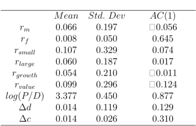
Table1 provides descriptive statistics for the continuously compounded returns on the assets, the market-wide price-dividend ratio, and the aggregate consumption and dividend growth rates for the annual sample over the period 1931_¬2009. The table illustrates the well documented equity premium and the size and value premia. Over the sample period, the annual equity premium over the risk free rate has mean 58%

and the volatility of the market return is 197%. The annual risk free rate has mean

08% and standard deviation 50%. The annual mean premium of small over large stocks is 47% and of value over growth stocks is 45%. Value stocks are much more volatile than growth stocks and small stocks are much more volatile than large stocks. The annual log price-dividend ratio on the market has a mean of338and standard error of 045over the sample period. The average annual log dividend growth rate on the market portfolio is14%with volatility119%. Finally, the annual log consumption growth has a mean of 14% and standard deviation of 26% over the sample period.

(11)

4 Forecasting Returns and Growth Rates

We pointed out in Section22that the LRR model of B-Y implies that the expected rate of return of the market, equity premium, dividend growth, and consumption growth are a¢ ne functions of the lagged price-dividend ratio and risk free rate. We test this implication of the model with in-sample linear forecasting regressions and out-of-sample linear predictive regressions. The in-out-of-sample forecasting tests are carried out at the monthly, quarterly, and annual frequencies and produces negative results, thereby ruling out the possibility that the model is rejected because it is interpreted at the wrong frequency. The out-of-sample predictability tests are carried out at the annual frequency and produce negative results which reinforce the in-sample results.

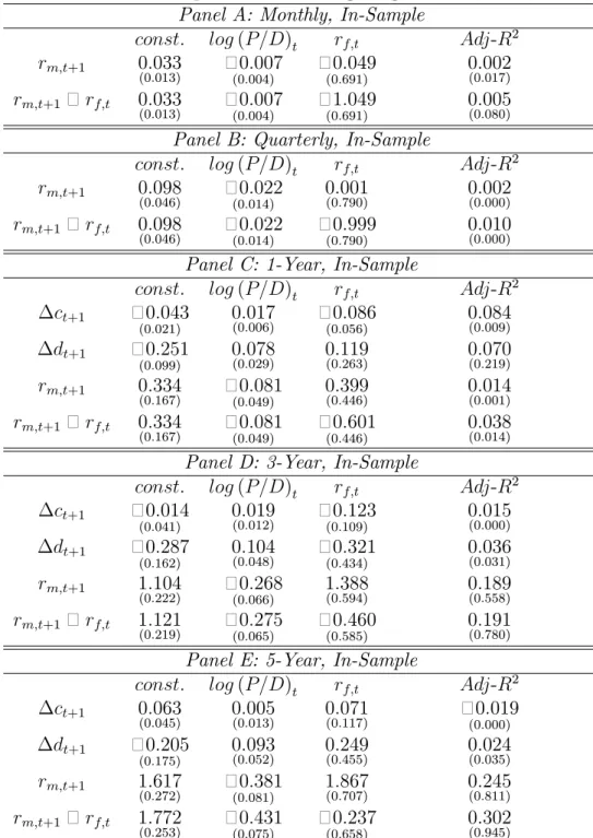
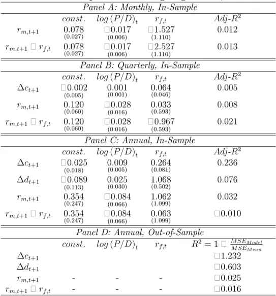
In Table 2, we report the results of in-sample linear forecasting regressions of the market return and equity premium at various frequencies over the full sample period

1931 : 1 through 2009 : 12. The regression coe¢ cients are uniformly statistically insigni…cant at the monthly, quarterly, and annual frequencies and the adjusted 2

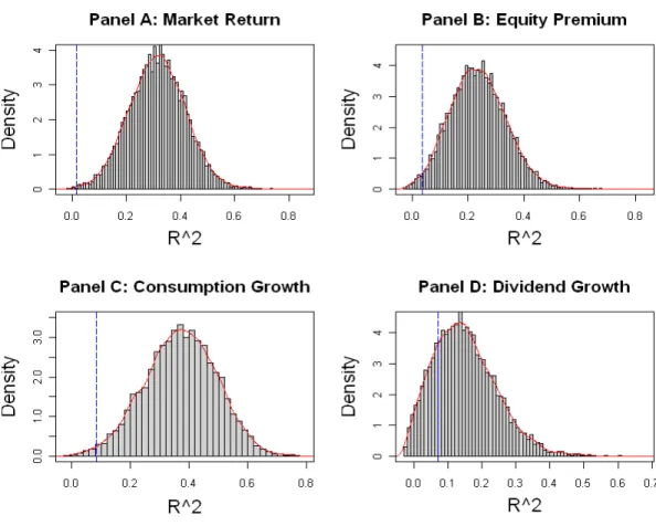
statistics are small as reported in Panels ¬ . In order to interpret the reported adjusted2 _{statistics, we calibrate and simulate the model. At the monthly frequency,}

we calibrate the model using the parameter values suggested by Bansal, Kiku, and Yaron (2007); at the quarterly and annual frequencies, we calibrate the model using the parameter values estimated by GMM and reported in Tables4and12, respectively. At each frequency, we generate10000 histories, run the in-sample forecasting regressions, and obtain the distributions of the adjusted2 _{statistics under the null hypothesis of}

the model. The distributions of the adjusted2 _{statistics at the annual frequency are}

displayed in Panelsand  of Figure1. In Table2and below each reported adjusted 2 _{statistic, we report in brackets the p-values that the model is correct. The p-values}

of the regressions of the market return and premium at all frequencies are lower than

2%, except for the p-value of the forecasting regression of the premium at the monthly frequency which is8%.3

In Table 2, Panels and , we also report the results of in-sample linear forecast-ing regressions of the market return and equity premium at 3- and 5-year horizons, respectively. Consistent with earlier results, we …nd that the price-dividend ratio and risk free rate perform well at forecasting the market return and equity premium at lower frequencies with the adjusted2 _{statistic varying from}₁₈__9%_to₃₀__2%_{. In order}

3_{Our results in Table} ₂_{, Panel} _ _{and Figure} ₁ _{di¤er from the results reported in Beeler and} Campbell (2009). Beeler and Campbell (2009) report results on in-sample linear forecasting regressions of the equity premium by the market-wide price-dividend ratio. They report a low2_{that is consistent}

to that implied by the model as inferred from simulations. Their results seem to contradict ours in Table2, Paneland Figure1. However, a crucial distinction between their forecasting regressions and ours is that we use both the price-dividend ratio and risk free rate as forecasting variables whereas they use only the price-dividend ratio. We do so because our theoretical discussion in Section2reveals that under the null, the expected equity return and premium are a¢ ne functions of both the price-dividend ratio and risk free rate.

(12)

to interpret the reported adjusted 2 statistics, we calibrate and simulate the model using the parameter values in Table 12. The p-values of the 2 _{statistics are high.}

In Table 3, Panels ¬, we report the corresponding results for the sub-period

1976 : 1 through 2009 : 12.4 _{The adjusted} _2 _{statistics are low or negative, with}

the exception of the regression of the market return at the annual frequency which has adjusted2 ₃__2%_{. Comparison of Table}₂_{, Panel}_ _{and Table}₃_{, Panel}__demonstrates

the instability of the results across subperiods. For the market return, the adjusted 2 _is ₁__4% _over _{1931 : 1}_¬ _{2009 : 12} _and ₃__2% _over _{1976 : 1}_¬ _{2009 : 12}_{. For the}

equity premium, the adjusted 2 _is ₃__8% _over _{1931 : 1}_¬_{2009 : 12} _{and negative over} 1976 : 1¬2009 : 12.

Additional evidence against the model comes from the out-of-sample prediction of the market return and equity premium. We evaluate the out-of-sample performance of these forecasts using an out-of-sample 2 _{statistic as in Campbell and Thompson}

(2008) and Welch and Goyal (2008).5 _{In Table} ₃_{, Panel} __{, we show that the}

mean-square-error statistics are negative which means that the predictive regression has higher mean-squared prediction error than the historical average return.

The strongest evidence against the model comes from the forecasting regressions for the aggregate consumption growth rate. We report the results of in-sample linear forecasting regressions of consumption growth for the full sample period only at the annual, 3-year, and 5-year frequencies because quarterly consumption data is only available since1947 : 1 (Table 2); and at the quarterly and annual frequencies for the sub-period 1976 : 1 through 2009 : 4 (Table 3). Over the full period, the adjusted 2 _{statistic of the consumption growth regression at the annual frequency is} ₈__4%

but the p-value is less than 1% (see Figure 1, Panel ) which means that the model of B-Y implies much higher predictability of consumption growth than the observed predictability. Likewise, the model implies much higher predictability of consumption growth at the 3-year, and5-year frequencies than that observed in the data.Over the post-war sub-period, the adjusted 2 _is ₂₃__6% _{in-sample but negative out-of-sample.}

Finally, we report the results of in-sample linear forecasting regressions of dividend growth at the annual,3-year, and5-year frequencies for the full sample period1931 : 1

4_{Our choice of the start date}_{1976 : 1} _{is motivated to coincide with the Welch and Goyal (}₂₀₀₈₎ comprehensive study on forecasting.

5_{We estimate the regression coe¢ cients over}_{1931 : 1}_¬_{1975 : 4}_{and predict the market return and} equity premium for the following year,1976 : 1_¬1976 : 4. We then enlarge the estimation window to

1931 : 1_¬1976 : 4and predict the market return and equity premium for the year1977 : 1_¬1977 : 4.

We repeat this procedure until2009. We impose two restrictions suggested in Campbell and Thompson (2008): …rst, we set the regression coe¢ cients to zero whenever they have the wrong sign (di¤erent from the theoretically expected sign estimated over the full sample); second, we set the forecast to the zero whenever it is negative. The out-of-sample performance of these forecasts is evaluated using an out-of-sample2 _{statistic: (}_2

 = 1¬  ), where denotes the mean-squared prediction

error from the predictive regression implied by the model and   denotes the mean-squared

(13)

through 2009 : 4 (Table 2); and at the annual frequency over the sub-period 1976 : 1

through2009 : 4(Table3). At the annual frequency, the results are positive. Over the full period, the adjusted 2 _is ₇__0% _{and the p-value of the model is} ₂₁__9% _{(see Figure} 1, Panel ). Over the post-war sub-period, the adjusted 2 is 76%. In the out-of-sample linear predictive regression at the annual frequency, however, the adjusted 2 _{is negative (Table} ₃_{, Panel} __{). Moreover, at the} ₃_{-year, and} ₅_{-year frequencies,}

the model implies much higher predictability of consumption growth at the 3-year, and 5-year frequencies than that observed in the data with p-values 31% and 35%, respectively.

Overall the results reported in this section provide robust time series evidence against the LRR model of B-Y in both the full period and the sub period and at all frequencies. In the next section, we address the implications of the model on the cross-section of returns.

5 Empirical Evidence on the Equity Premium and

the Cross-Section of Returns

5.1 Methodology

First, we estimate the time-series parameters of aggregate consumption and dividend growth without reference to the Euler equations. We choose the nine parameters of the time-series model (1)-(4) to match the following nine sample moments: the uncon-ditional mean, variance, and …rst-order autocorrelation of consumption and dividend growth rates, the correlation between consumption and dividend growth rates, and the variance of squared consumption and dividend growth rates. These estimates are re-ported in Section52 and serve as a benchmark for comparison when we subsequently re-estimate them from the joint system of time-series moment restrictions and Euler equations.

In Sections 53 and 54, we address the equity premium and the cross-section of returns, respectively. The system of equations consists of the Euler equations of con-sumption on a given set of assets along with the restrictions imposed on the model parameters by the unconditional moments of the aggregate consumption and dividend growth which we described above. We estimate the parameters with GMM using the e¢ cient weighting matrix and test the model with the overidentifying restrictions. We verify the robustness of the tests by replacing the e¢ cient weighting matrix with the identity matrix. The tests are carried out at the annual frequency. Later on, we test the robustness of the tests by repeating them at the quarterly frequency and in subperiods. In Section53, the set of assets consists of the market portfolio and the risk free rate, thereby focusing on the equity premium and the risk free rate puzzles. We introduce

(14)

two unconditional Euler equations for the market portfolio and the risk free rate along with four Euler equations for the market portfolio and the risk free rate conditional on the lagged log price-dividend ratio of the market and the lagged log risk free rate. To this set of pricing restrictions we append the nine moment restrictions implied by the time-series speci…cation of the model which we stated earlier. Thus, we have a total of15moment conditions. The total number of parameters to be estimated is 12, consisting of nine time-series parameters and three preference parameters. In Section

54, the set of assets consists of the "Value", "Growth", "Small" capitalization, and "Large" capitalization stocks, in addition to the market portfolio and the risk free rate. The Euler equations for these six assets along with the nine time-series moment restrictions give15 moment restrictions in 12parameters. The numerical search for a global minimum is described in Appendix5.

5.2 Time-Series Properties of Aggregate Consumption and

Dividend Growth

In Table4under the label “Data”, we display the sample averages of the nine moments of the consumption and dividend growth rates which we aim to match. The nine para-meters of the time-series model (1)-(4) are chosen such that the nine model-generated moments, as displayed under the adjacent column labeled " _{", exactly match}

their sample averages. This is feasible because the model is just identi…ed. The point estimates of the nine model parameters, along with the associated standard errors in parentheses, are displayed in the …rst row of the table.6 The persistence parameter ( _) of the LRR variable is 032 and is statistically signi…cantly positive at conven-tional levels of signi…cance. This lends support to the major risk channel highlighted in the LRR literature— a predictable component in the aggregate consumption and dividend growth rates.

5.3 Evidence on the Equity Premium

We address the equity premium and risk free rate puzzles by introducing two uncon-ditional Euler equations for the market portfolio and the risk free rate along with four Euler equations conditional on the lagged log price-dividend ratio of the market and the lagged log risk free rate. Combined with the nine time-series moment restrictions, this system of15restrictions and12parameters (9time-series parameters plus3preference parameters) is overidenti…ed. The results are displayed in Table 4.

The GMM overidentifying restrictions test rejects this model with J-stat 177 and 6_{The standard errors are Newey-West corrected using two lags.}

(15)

asymptotic p-value less than 1%.7 _{The annual pricing error for the risk free rate is}

¬33% and is economically signi…cant. The annual pricing error for the market return is¬19%.

The second row of Table 4 displays the point estimates of the time-series and preference parameters when both the pricing restrictions and the time-series restrictions are used in the estimation. The risk aversion estimate is8which is reasonable although the standard error is large at 659. The point estimate of the IES is 06; however the standard error is 133and we cannot reject the hypothesis that the elasticity exceeds the value of one.

The persistence parameter of the LRR variable is much higher at 070, compared to the value of032estimated from the time-series model alone. This suggests that the B-Y model requires much higher predictability of consumption growth to explain the equity premium and risk free rate puzzles than the predictability estimated from the time series of consumption growth alone.

5.4 Evidence on the Cross-Section of Returns

In Table 5, we report the results of tests on the cross-section of returns consisting of the "Value", "Growth", "Small" capitalization, and "Large" capitalization stocks, in addition to the market portfolio and the risk free rate.

The results reinforce the conclusions drawn from the 2-asset system. As in the two-asset system, the GMM test rejects this model with J-stat136 and asymptotic p-value less than1%. The annual pricing errors for the market return, “Large”portfolio, "Value" portfolio, and risk free rate are small. The annual pricing errors for the “Small” and “Growth”portfolios are larger at 26% and _¬29%, respectively. The estimates of the risk aversion and the IES are remarkably similar to the corresponding estimates in the2-asset system. As in the 2-asset system, the B-Y model requires much higher predictability of consumption growth to explain the cross-section of returns than the predictability estimated from the time series of consumption growth alone.

6 A co-integrated Long Run Risks Model

Bansal, Gallant, and Tauchen (2007) consider a variant of the LRR model of B-Y that imposes a co-integrating restriction between the logarithm of the aggregate stock market dividends and consumption. Bansal, Dittmar, and Kiku (2007) point out that this co-integrating relation measures long run covariance risks in dividends and is im-portant in understanding sources of risk and explaining the equity risk premia across 7_{Note that the J-stat has an asymptotic chi-squared distribution with}₃_{degrees of freedom under} the null.

(16)

investment horizons.8 _{We consider a log-linearized variant of the Bansal, Gallant, and}

Tauchen (2007) model that yields closed-form expressions for asset prices. We estimate and test the model using an extension of the methodology introduced in Section 2.

6.1 The Model and Testable Implications

The aggregate consumption growth, the LRR variable, and the variance of its inno-vation are modeled as in equations (1)-(3). Therefore, the pricing kernel, the log price-consumption ratio, and the risk free rate are functions of the LRR variable and the variance of its innovation, given by equations (19), (10), and (12), respectively.

The point of departure is the imposition of a co-integrating restriction between the logarithm of the aggregate stock market dividends and consumption,

¬= +, (21)

where the cointegrating residual,, is an(0)process with the cointegrating coe¢ cient

set at one,9

+1 = + +  +1. (22)

The shocks +1, +1,  +1, and +1 are assumed to be  (01) and

mutually independent.

From equation (21), we have,

+1 = +1+ +1 (23)

= _ + (1 + )+ ( ¬1)+ +1+  +1,

where the second line follows from equations (3) and (22).

The model has three state variables, the LRR variable, the variance of its innovation, and the co-integrating residual. Note that the B-Y model obtains as a limiting special case when _ = 1. We conjecture that the log price-dividend ratio is an a¢ ne function of the state variables,

 =0+1+2 2 +3. (24)

In Appendix31, we verify this conjecture and explicitly solve for the coe¢ cients. 8_{In a di¤erent context, Lettau and Ludvigson (}₂₀₀₁_{) and Menzly, Santos, and Veronesi (}₂₀₀₄₎ apply the co-integrating residual between consumption, labor income, and aggregate stock market dividends to explain the cross-section of returns.

9_{Bansal, Gallant, and Tauchen (}₂₀₀₇_{) perform a heteroskedasticity-robust augmented Dickey-Fuller} test for a unit root in¬and the results provide strong evidence for a cointegrating relationship

(17)

The co-integrating residual is observable as the demeaned di¤erence between the log aggregate dividend and consumption levels (see equation (21)). We invert equations (12) and (24) and express the unobservable state variables, and 2, in terms of the

observables, , , and , (see Appendix 32 for details and expressions for 0,

1, 2, 3, 0, 1, 2 and 3),

 = 0+ 1+ 2+ 3, (25)

2

 = 0+ 1+ 2+ 3. (26)

Equations (9), (24), (25), (26), and (12) imply that the expected market return and equity premium are a¢ ne functions of the state variables. Furthermore, it is straightforward to see that the expected consumption and dividend growth rates are a¢ ne functions of the state variables. Since the state variables,  and 2 are a¢ ne

functions of the observables , , and , we may express the expected market

return, equity premium, dividend growth, and consumption growth as a¢ ne functions of the observables , , and , with coe¢ cients known functions of the model

parameters. In the next section, we test the predictive implications of the model through in-sample linear forecasting regressions and out-of-sample linear predictive regressions of the market return, equity premium, dividend growth, and consumption growth on the lagged price-dividend ratio, risk free rate, and the di¤erence between the log dividend and consumption levels.

Finally, we derive the pricing implications of the model. Using equations (7), (8), and (10), we write the pricing kernel as,

+1 = ( log + ( ¬1) [ 0+ ( 1¬1)0]) + ¬ + ( ¬1) +1 +( _¬1) 11+1+ ( ¬1) 12 2+1

¬( _¬1)1¬( ¬1)2 2, (27)

Substituting the expressions forand 2 from equations (25) and (26) into equation

(27), we express the pricing kernel entirely in terms of observables (see Appendix32

for details), +1 =1+2 +1+3 +1¬ 1 1  +4 +1¬ 1 1  +5 +1¬ 1 1  . (28) In the next section, we …rst examine the empirical plausibility of the model when the asset menu consists of the market portfolio and the risk free rate. The lagged log price-dividend ratio of the market and the lagged log risk free rate are used as

(18)

instruments. The Euler equations for the two assets along with the two chosen in-struments give 6 moment restrictions. To this set of pricing restrictions, we add moment restrictions implied by the time-series speci…cation of the model. In par-ticular, we include the following 7 moments of consumption and dividend growth rates: ( +1),  ( +1), ( +1 +2), ( +1 +3),  ( +1),

( +1 +2), and ( +1 +1) (see Appendix A.4 for expressions for

these moments in terms of the time-series parameters). Thus, we have a total of 13 moment conditions. The total number of parameters to be estimated is 12, including 9 time-series parameters and 3 preference parameters. We estimate the parameters with GMM and test the speci…cation of the model using the overidentifying restriction.

We then examine the ability of the model to explain the cross-section of returns. In this case, the asset menu consists of the market portfolio, the risk free rate, and portfolios of "Small" capitalization, "Large" capitalization, "Growth" and "Value" stocks. The Euler equations for the 6 assets give 6 moment restrictions. To this set of pricing restrictions, we add the 7 moment restrictions implied by the time-series speci…cation of the model. This gives, once again, a total of 13 moment conditions in 12 parameters. We estimate the parameters and test the model speci…cation with GMM.

6.2 Empirical Evidence on the Co-integrated Model

In Table6, we report the results of in-sample linear forecasting regressions of the market return, equity premium, and the consumption and dividend growth rates at the annual frequency for the full sample period1931through2009. We do not report results at the monthly and quarterly frequencies because reliable data on the co-integrating residual, the demeaned di¤erence between the log aggregate dividend and consumption levels, is not available at the monthly frequency and is only available for the postwar subperiod at the quarterly frequency. In Table 7, Panels  and , we report the corresponding results at the quarterly and annual frequencies, respectively, for the sub-period1976 : 1

through2009 : 4.

Tables 6 and 7 reveal that the di¤erence between the log aggregate dividend and consumption levels,, has substantial incremental forecasting power for the aggregate

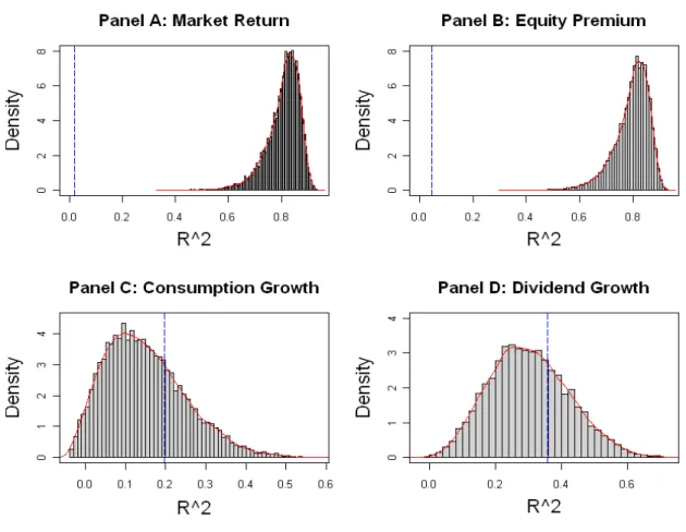
consumption and dividend growth rates over and above that contained in the log price-dividend ratio and risk free rate at the annual and quarterly frequencies. In-sample forecasting regressions for the consumption growth rate have adjusted-2 ₁₉__8% _and

p-value713%over the full period (Table6, Row1and Figure2, Panel) and adjusted-2 ₃₈__3% _{over the subperiod (Table}₇_{, Panel} __{, Row}₁_{) at the annual frequency. The}

coe¢ cient of  is statistically signi…cant in both cases. Similar results are obtained

for the aggregate dividend growth rate for which the adjusted-2 _is ₃₅__6% _{and the}

(19)

adjusted-2 is151%over the subperiod (Table7, Panel, Row2). However, Table7, Panel reveals that the state variables of the co-integrated model fail to retain their predictive power for consumption and dividend growth rates of-sample. The out-of-sample2 for the consumption growth rate is _¬517% and for the dividend growth rate _¬237%.

The state variables do not forecast the market return and equity premium as pre-dicted by the co-integrated model. At the annual frequency and over the full period, the adjusted-2 _{for the market return is} ₂__0% _(Table ₆_{, Row} ₃_{) and for the equity}

premium is44%(Table6, Row4). However, the p-values of these regressions are zero, meaning that the co-integrated model implies much higher predictability of the market return and equity premium using the market-wide price-dividend ratio, risk free rate, and the demeaned dividend-consumption ratio than the observed predictability (see Figure2, Panels  and ).

Furthermore, the observed predictability by the state variables of the co-integrated model is unstable. At the annual frequency over the 1976 ¬ 2009 sub-period, the adjusted-2 _{for the market return is} ₀__0% _(Table ₇_{, Panel} __{, Row} ₃_{) and for the}

equity premium is negative (Table 7, Panel , Row 4). Given the poor in-sample forecasting performance of the model-implied state variables, it is not surprisingly the out-of-sample 2 _{for the market return and equity premium are} _¬₅__5% _and _¬₅__0%_,

respectively (Table 7, Panel , Rows 3 and 4). At the quarterly frequency over the

1976¬ 2009 sub-period, the adjusted-2 _{for the market return is negative (Table} ₇_,

Panel, Row 3) and for the equity premium is10% (Table 7, Panel , Row4). The pricing implications of the model for the 2-asset system are displayed in Table8. The point estimate of the auto-correlation coe¢ cient, _, of the co-integrating residual, , is 096 and the asymptotic standard error is 076. Therefore, the data cannot

distinguish the co-integrated model from the B-Y model which obtains as a limiting special case when _ = 1. This explains why the conclusions drawn from Table 8 are similar to our earlier conclusions from Table 4. Speci…cally, the persistence parameter of the LRR variable is much higher at 094, compared to the value of 032 estimated from the time-series model alone in Table4. Therefore, the co-integrated model, as the B-Y model, requires much higher predictability of consumption growth to explain the equity premium and risk free rate puzzles than the predictability estimated from the time series of consumption growth alone. The GMM overidentifying restrictions test rejects this model with J-stat 919 and asymptotic p-value less than 1%. The point estimates of the parameters are similar to those in Table 4. The annual pricing error for the risk free rate is 29% and for the market return is 15%.

The pricing implications of the model for the6-asset system are displayed in Table9. The point estimate of the auto-correlation of the co-integrating residual is090and the asymptotic standard error is130. As in the2-asset system, the data cannot distinguish the co-integrated model from the B-Y model and the conclusions drawn from Table

(20)

model, as the B-Y model, requires much higher predictability of consumption growth to explain the cross-section of returns than the predictability estimated from the time series of consumption growth alone. The GMM overidentifying restrictions test rejects this model with J-stat912and asymptotic p-value less than 1%. The point estimates of the parameters are very similar to those in Table 5. The annual pricing errors for the “Small” portfolio (43%) and “Value” portfolio (32%) are economically large.

The co-integrated LLR model generalizes the LRR model of B-Y by introducing the di¤erence between the log dividend and consumption levels as a third state variable. The combined evidence from the out-of-sample predictive regressions and the pricing tests suggest that the problems identi…ed with the model of B-Y remain to be resolved.

7 Robustness Tests

In Section71, we address the robustness of our results to the post-war sub-period. In Section72, we explore the pricing implications of the B-Y model at the quarterly, as opposed to the annual, frequency.

7.1 Robustness to the Post-War Sub-Period

Since the period prior to 1947 was one of great economic uncertainty, including the Great Depression, World War II, and structural breaks in the equity premium, rejection of the LRR models in the full sample may be due to their poor performance in the pre-war period. Pastor and Stambaugh (2001) document evidence of breaks in the equity premium in the early thirties and forties, and in the early and mid-nineties. Lettau, Ludvigson, and Wachter (2008) …nd evidence of a break in the consumption variance around1992, followed by a break in the log price-dividend ratio of the market around

1995. Lettau and Van Nieuwerburgh (2008) report evidence of two breaks in the mean of the aggregate price-dividend ratio around1954 and 1994.

We explore the possibility that rejection of the LRR model of B-Y and its co-integrated extension is due, in part, to failure to account for regime shifts over the period1931¬2009. In Section 4, we already provide evidence that the lack of out-of-sample predictability of the market return, equity premium, consumption growth, and dividend growth in linear regressions on the price-dividend ratio and risk free rate over the period 1931¬ 2009 (Table 2) persists over the sub-period 1976¬2009 (Table 3). In Section 6, we add the di¤erence between the log dividend and consumption levels as a third predictive variable, as implied by the LRR model of Bansal, Gallant, and Tauchen (2007), and provide evidence that the lack of out-of-sample predictability over the period 1931_¬2009 (Table 6) persists over the sub-period 1976_¬2009 (Table 7).

As further evidence of the robustness of our results we present estimation and test results of the Euler equations of consumption over the post-war sub-period1947¬2009

(21)

on the2-asset system (Table10) and the6-asset system (Table11). The model is still rejected on both the2-asset and6-asset systems with p-values less than1%. The point estimates of the parameters and the pricing errors are similar in the full period and the post-war sub-period and lend support to the robustness of the empirical methodology.

7.2 Interpretation of the Model at the Quarterly Frequency

We explore the possibility that the LRR model of B-Y applies at the quarterly, as opposed to the annual, frequency. The lack of out-of-sample predictability of the market return, equity premium, dividend growth, and consumption growth reported in Section 4 cannot be attributed to the possibility that the LRR model of B-Y applies at the quarterly, as opposed to the annual, frequency because the tests are carried out at both the quarterly and annual frequencies.

Our rejection of the Euler equations of consumption on the 2-asset and 6-asset systems at the annual frequency is susceptible to the criticism that the LRR model applies at the quarterly frequency and the Euler equations stated at the annual fre-quency improperly temporally aggregate consumption ‡ows. Therefore, we repeat our estimation and tests of the Euler equations at the quarterly frequency. Since reliable quarterly data are only available over the post-war sub-period, we perform our tests over1947 : 2¬2009 : 4. Tables12and13display the results for the2-asset and6-asset systems, respectively. The annualized pricing errors are very similar to those obtained using annual data over the post-war subperiod.

The results in this section suggest that our …ndings are unlikely to be driven by the problems associated with temporal aggregation or by the interpetation of the model at the wrong frequency.

8 Concluding Remarks

We present a novel methodology in testing the long-run risks model of Bansal and Yaron (2004) based on the observation that, under the null, the potentially latent state variables, “long-run risk” and the conditional variance of its innovation, are known a¢ ne functions of the observable market-wide price-dividend ratio and risk free rate.

Using the methodology, we test the time-series and cross-sectional pricing impli-cations of the model over the sample period 1931¬ 2009. The results are robust to the interpretation of the model at the annual, quarterly, and monthly frequencies; to the full time period 1931_¬ 2009 versus the post-war sub-period; to the temporal ag-gregation of consumption ‡ows; and to the co-integration or lack of co-integration of the consumption and dividend levels. Whereas we formally reject the model, we derive valuable insights which should prove useful in guiding future search.

(22)

much more forecastable by the price-dividend ratio and risk free rate in linear regres-sions than what we observe in the data. What may be needed is a richer model in which the expected market return, equity premium, consumption growth, and pricing kernel are nonlinear functions of the two state variables. Alternatively, what may be needed is a model that introduces a third state variable that plays a major role in forecasting the expected market return, equity premium, and consumption growth and also plays a major role in explaining the cross-section of returns. The observed di¤erences in the results between the full sample period and the post-war sub-period reinforce the view that the economy experiences structural breaks which may be fruitfully captured by such a state variable.

(23)

A

Appendix

A.1 Estimation of Time-Series Parameters

The decision interval of the agent is assumed to be annual. We estimate the model at the annual frequency, such that its annual growth rates of consumption and dividends match salient features of observed annual consumption and dividend data. There are 9 parameters to be estimated - _, _, , , _, _, , , and .

From the speci…cation of the consumption growth process, we have

( +1) =  (29) We also, have  ( +1) =  () + ( +1) + 2( +1) =  () + 2+ 0 = 2  2 1_¬ 2  + 2 (30) and, ( +1 +2) =  2  2 1¬ 2  (31) From the speci…cation of the dividend process, we have

( +1) =  (32)  ( +1) = 2 2  2 1¬ 2  + 2_2 ₍₃₃₎ ( +1 +2) = 2  2  2 1_¬ 2  (34) Also, from the consumption and dividend growth processes,

( +1 +1) = 2  2 1¬ 2  (35) Finally, we have

(24)

 ¬( +1)2 =   ¬ ( +1)2 +   ¬ ( +1)2 (36) Now, ( +1)2 = 2 +2 + 2+1+ 2 + 2 +1+ 2  +1 (37) Hence,  ¬ ( +1)2 = 2 +2 + 2 + 2     ¬ ( +1)2 =  (2) + ( 2) + 4 2 () + 4 ( 2) +2(2_ 2_) + 4 _( 2) (38) Now,  ( 2 ) = 2  1¬ 2, ( 2) = 0, (2 2) = 2  2 (1¬ 2₎₍₁_¬ 2 ), (  2 ) = 0, and  (2_) = 3 4  2(1 + 2) (1_¬ 4 )(1¬ 2)(1¬ 2) + 1 1_¬ 4  2 4+ 4 2  4 4 (1_¬ 2 )

Substituting the above expressions into equation (38), we have

   ¬ ( +1)2 = 3 4_ 2 (1 + 2) (1_¬ 4 )(1¬ 2)(1¬ 2) + 1 1_¬ 4  2 4+ 4 2  4 4 (1_¬ 2 ) + 2  1_¬ 2 + 4 2  2  2 1_¬ 2  + 2 2  2 (1_¬ 2₎₍₁_¬ 2 ) (39) Also, from equation (37),

  ¬ ( +1)2 = 2 4 + 42 2 + 4 2 2 + 8  2 Hence,    ¬ ( +1)2 = 2 2  1¬ 2 + 2 4 ₊ 4 2 2 (1¬ 2₎₍₁_¬ 2 ) + 4 2  4 1¬ 2  + 4 2_ 2 (40) Substituting equations (39) and (40) into equation (36), we have

 ¬( +1)2 = 3 4_ 2 (1 + 2) (1_¬ 4 )(1¬ 2)(1¬ 2) + 1 1_¬ 4  2 4+ 4 2  4 4 (1_¬ 2 ) + 3 2  1_¬ 2 +4 2_ 2  2 1_¬ 2  + 6 2  2 (1_¬ 2₎₍₁_¬ 2 ) + 4 2  4 1_¬ 2  + 2 4+ 4 2_ 2 (41)

(25)

Similar calculations yield,    ¬ ( +1)2 = 4 3 4_ 2 (1 + 2) (1_¬ 4 )(1¬ 2)(1¬ 2) + 1 1_¬ 4  2 4+ 4 2  4 4 (1_¬ 2 ) + 2  1_¬ 2 4_{+ 4} 2  2  2 1_¬ 2  2 ₊ 2 2  2 (1_¬ 2₎₍₁_¬ 2 ) 2_2    ¬ ( +1)2 = 2 2  1¬ 2 + 2 4 _4₊ 4 2 2 (1¬ 2₎₍₁_¬ 2 ) + 4 2  4 1¬ 2  2_2 +4 2 2 2 Hence, we have  ¬( +1)2 = 4 3 4_ 2 (1 + 2) (1¬ 4 )(1¬ 2)(1¬ 2) + 1 1¬ 4  2 4+4 2  4 4 (1¬ 2 ) + 3 2  1¬ 2 4 +4 2_ 2  2 1_¬ 2  2₊ 6 2 2 (1_¬ 2₎₍₁_¬ 2 ) 2_2₊ 4 2 4 1_¬ 2  2_2 +2 44+ 4 2_2 2 (42)

Equations (29)-(35), (41), and (42) give 9 moments restrictions in the 9 time-series parameters.

A.2 Details of Estimation Methodology

The model is given by the equations

+1 = +  +1,

2

+1 = (1¬ ) 2+ 2 +  +1,

+1 =  ++ +1,

+1 = + x+' +1.

The shocks +1,  +1, +1, +1 are assumed to be  (01) and mutually

(26)

A.2.1 Expressions for A₀, A₁, A₂, A₀_, A₁_, and A₂_

Bansal and Yaron (2004) show that  and , are a¢ ne functions of the state

vari-ables,  and 2,  = 0+1+2 2,  = 0+1+2 2, where 1 = 1¬ 1 1¬ 1  2 = 05 _¬ + 2+ ( 11 ) 2 (1_¬ 1 ) 0 = ( ) + 1_¬ 1 + 0+ 12 2(1¬ ) + 05 12 2 1_¬ 1 1 = ¬ 1 1¬ 1  2 = (1_¬ )2(1¬ 1 ) + 05 2+2+ (( ¬1) 11+ 11)2 2 1¬ 1 0 = log( ) + _¬ + _¬1 _ + ( _¬1) 0 + ( ¬1) ( 1¬1)0+ ( ¬1) 12 2(1¬ ) 1_¬ 1 + 0+ + 12 2₍₁_¬ _{) + 0}__{5 [(} _¬₁₎ 12+ 12]2 2 1_¬ 1

A.2.2 Risk Free Rate

To derive the expression for the risk free rate, note that

 exp log ¬ +1+ ( ¬1)+1+ = 1

(27)

exp (_¬) =  exp log ¬ +1+ ( ¬1)+1 = exp( log ¬ ¬ + ( ¬1) 0+ ( ¬1) 10 +( _¬1) 11 + ( ¬1) 12(1¬ ) 2+ ( ¬1) 12 2 ¬( ¬1)0¬( ¬1)1¬( ¬1)2 2 + ( ¬1) + ( ¬1) +05 " ¬ + _¬1 2 2  + ( ¬1)2 2121 2 2 + ( ¬1)2 2122 2 # )

Therefore, the risk free rate is

 = ¬ log ¬ ¬ + ¬1 ¬( ¬1) 0¬( ¬1)( 1¬1)0¬( ¬1) 12(1¬ ) 2 ¬05( ¬1)2 2₁2₂ 2_ ¬ (¬ + ¬1) + ( ¬1)( 1 ¬1)1  ¬ " ( _¬1)( 1 ¬1)2+ 05 ¬ + ¬1 2 + ( _¬1)2 2₁2₁ 2_ !# 2  = 0 +1+2 2 where 0 = ¬ log ¬ ¬ + ¬1 ¬( ¬1) 0¬( ¬1)( 1¬1)0¬( ¬1) 12(1¬ ) 2 ¬05( ¬1)2 2122 2 1 = ¬ (¬ + ¬1) + ( ¬1)( 1 ¬1)1 2 = ¬ " ( _¬1)( 1 ¬1)2+ 05 ¬ + ¬1 2 + ( _¬1)2 2₁2₁ 2_ !#

A.2.3 Latent state variables in terms of observable variables

The model implies

 = 0+1+2 2,

(28)

These equations may be inverted to express the state variables in terms of the observables, = 0+ 1+1+ 2, where 0 = 20 ¬02 12 ¬21 , 1 = ¬ 2 12 ¬21 , 2 = 2 12 ¬21 , and 2  = 0+ 1+1+ 2, where 0 = 01 ¬10 12 ¬21 , 1 = 1 12 ¬21 , 2 = ¬ 1 12 ¬21 .

A.2.4 The pricing kernel in terms of observables

The pricing kernel is given by (19),

+1 = ( log + ( ¬1) [ 0+ ( 1¬1)0]) + ¬ + ( ¬1) +1 +( _¬1) 11+1+ ( ¬1) 12 2+1¬( ¬1)1¬( ¬1)2 2

Substituting the expressions forand 2 from Section A.1.2 into the pricing kernel,

we have +1 =1+2 +1+3 +1¬ 1 1  +4 +1¬ 1 1 

(29)

where

1 = log + ( ¬1)[ 0+ ( 1¬1) (0+1 0+2 0)]

2 = ¬ + ( ¬1)

3 = ( ¬1) 1[1 1+2 1]

4 = ( ¬1) 1[1 2+2 2]

A.3 Estimation Methodology for co-integrated Model

The model is given by the equations

+1 =  ++ +1, +1 = +  +1, 2 +1 = + 2 +  +1, ¬ = +, +1 = + +  +1, +1 =  + (1 + )+ ( ¬1)+ +1+  +1. (43)

A.3.1 The Dividend Claim

We conjecture that the log price-dividend ratio is an a¢ ne function of the state vari-ables, , 2, and :

 =0+1+2 2 +3.

The coe¢ cients 0, 1, 2, and 3 are computed using the method of

unde-termined coe¢ cients as described below.

The Euler equation for the observable return on the aggregate dividend claim, +1, is,

 exp log ¬ +1+ ( ¬1)+1++1 = 1 (44)

Substituting the expression for +1 from equation (9) into the above Euler

(30)

[exp( log ¬ ¬ ¬ +1+ ( ¬1) 0+ ( ¬1) 10 +( ¬1) 11 + ( ¬1) 11  +1 +( _¬1) 12 + ( ¬1) 12 2 + ( ¬1) 12  +1 +( _¬1) 13 + ( ¬1) 13 + ( ¬1) 13  +1 ¬( _¬1)0¬( ¬1)1¬( ¬1)2 2 ¬( ¬1)3 +( ¬1)  + ( ¬1)+ ( ¬1) +1 + 0+ 10+ 11 + 11  +1+ 12 + 12 2 + 12  +1+ 13 + 13  + 13  +1¬0¬1¬2 2 ¬3 + _ + (1 + )+ ( ¬1)+ +1+  +1)] = 1

Using the assumed conditional log-normality of the stochastic processes, the left-hand-side of the above expression simpli…es to

exp( log + _¬ + _+ ( _¬1) 0+ ( ¬1) ( 1¬1)0+ ( ¬1) 12 + 0+ ( 1¬1)0+ 12 + ¬ + ¬1 + ( ¬1) ( 1 ¬1)1+ ( ¬1) 13 + ( 1 ¬1)1+ (1 + )  + [ 13 ]+ [( ¬1) ( 1 ¬1)3+ ( 1 ¬1)3+ ¬1] + [( _¬1) ( 1 ¬1)2+ ( 1 ¬1)2] 2 +05_{f ¬} + 2 2  + [( ¬1) 13+ 13+ 1]2 2 2 + [( ¬1) 11+ 11]2 2 2 + [( ¬1) 12+ 12]2 2g) = 1 (45)

Since the Euler equation (45) must hold for all values of the state variables, we have

[( ¬1) ( 1 ¬1)3+ ( 1  ¬1)3+ ¬1] = 0 3= ¬ 1 1_¬ 1  (46) ¬ + _¬1 +( _¬1) ( 1 ¬1)1+( ¬1) 13 +( 1 ¬1)1+ 13 +1+  = 0

(31)

1= 1_¬ 1 ₊ (1 + 13) 1_¬ 1  (47) ( _¬1) ( 1 ¬1)2+ ( 1 ¬1)2+ 05f ¬ + 2 + [( ¬1) 13+ 13+ 1]2 2+ [( ¬1) 11+ 11]2 2g = 0 2 = ( _¬1) ( 1 ¬1)2+ 1¬ 1 (48)  = 05f ¬ + 2 + [ 13+ 1]2 2 + [( _¬1) 11+ 11]2 2g log + _¬ + _+ ( _¬1) 0+ ( ¬1) ( 1¬1)0+ ( ¬1) 12 + 0+ ( 1¬1)0+ 12 + 05 [( ¬1) 12+ 12]2 2 = 0 0 = log + _¬ + _+ ( _¬1) 0+ ( ¬1) ( 1¬1)0 1_¬ 1 (49) +( ¬1) 12 + 0+ 12 + 05 [( ¬1) 12+ 12] 2 2  1¬ 1

A.3.2 Latent State Variables in terms of Observable Variables

We have

 = 0+1+2 2 +3

 = 0 +1+2 2

The above equations may be inverted to express the unobservable state variables,  and 2, in terms of the observables,,, and .

(32)

De…ne,  12 ¬12 We have,  = 0+ 1+ 2+ 3 0 = 02¬02  1 = ¬ 2  2 = 2  3 = ¬ 32  2  = 0+ 1+ 2+ 3¬ 0 = 01 ¬10  1 = 1  2 = ¬1  3 = 13 

Now, from equations (7), (8), and (10), the pricing kernel is given by the expression

+1 = ( log + ( ¬1) [ 0+ ( 1¬1)0]) + ¬ + ( ¬1) +1 +( ¬1) 11+1+ ( ¬1) 12 2+1

¬( _¬1)1¬( ¬1)2 2

Substituting the expressions for  and 2 from equations (25) and (26) into the

above expression for the pricing kernel, we have

+1 =1+2 +1+3 +1¬ 1 1  +4 +1¬ 1 1  +5 +1¬ 1 1 