Full text document (pdf)
Copyright & reuse
Content in the Kent Academic Repository is made available for research purposes. Unless otherwise stated all content is protected by copyright and in the absence of an open licence (eg Creative Commons), permissions for further reuse of content should be sought from the publisher, author or other copyright holder.
Versions of research
The version in the Kent Academic Repository may differ from the final published version.
Users are advised to check http://kar.kent.ac.uk for the status of the paper. Users should always cite the published version of record.
Enquiries
For any further enquiries regarding the licence status of this document, please contact: researchsupport@kent.ac.uk
If you believe this document infringes copyright then please contact the KAR admin team with the take-down information provided at http://kar.kent.ac.uk/contact.html
Citation for published version
Hao, MingJie and Macdonald, Angus S. and Tapadar, Pradip and Thomas, R. Guy (2016) Insurance
loss coverage and demand elasticities. Working paper. Unknown (Submitted)
DOI
Link to record in KAR
http://kar.kent.ac.uk/59795/
Document Version
UNSPECIFIED
INSURANCE LOSS COVERAGE AND DEMAND ELASTICITIES
By MingJie Hao, Angus S. Macdonald , Pradip Tapadarand R. Guy Thomas
abstract
Restrictions on insurance risk classification may induce adverse selection, which is usually per-ceived as a bad outcome. We suggest a counter-argument to this perception in circumstances where modest levels of adverse selection lead to an increase in ‘loss coverage’, defined as expected losses compensated by insurance for the whole population. This happens if the shift in coverage towards higher risks under adverse selection more than offsets the fall in number of individuals insured. The possibility of this outcome depends on insurance demand elasticities for higher and lower risks. We state elasticity conditions which ensure that for any downward-sloping insur-ance demand functions, loss coverage when all risks are pooled at a common price is higher than under fully risk-differentiated prices. Empirical evidence suggests that these conditions may be realistic for some insurance markets.
keywords
Adverse selection; loss coverage; elasticity of demand; arc elasticity of demand.
contact address
School of Mathematics, Statistics and Actuarial Science, University of Kent, Canterbury, CT2 7NF, UK.
Department of Actuarial Mathematics and Statistics, and the Maxwell Institute for Mathemat-ical Sciences, Heriot-Watt University, Edinburgh EH14 4AS, UK.
Corresponding author: R. Guy Thomas, R.G.Thomas@kent.ac.uk.
1. Introduction
Restrictions on insurance risk classification are common in life and health insurance markets. In the US, the Patient Protection and Affordable Care Act permits classification only by age, location, family size and smoking status; in the European Union, gender classification in insurance pricing has been banned; and many countries have restricted insurers’ use of genetic test results. Whilst such restrictions appear motivated by social objectives, they may also induce adverse selection, which is usually perceived as a bad outcome.
A simple version of the usual argument is as follows. If insurers are not permitted to charge risk-differentiated prices, they have to pool different risks at a common pooled
price. This pooled price is cheap for higher risks and expensive for lower risks; so more insurance is bought by higher risks, and less insurance is bought by lower risks. The equilibrium pooled price of insurance is higher than a population-weighted average of true risk premiums. Also, in most markets the number of higher risks is smaller than the number of lower risks, so the total number of risks insured falls.
However, the rise in equilibrium price under pooling reflects a shift in coverage towards higher risks. If the shift in coverage is large enough, it can more than offset the fall in numbers insured. In these circumstances, despite fewer risks being insured under pooling, expected losses compensated by insurance – a quantity we term ‘loss coverage’ – can be higher. We argue that where risk classification restrictions lead to higher ‘loss coverage’ – that is, more risk being voluntarily transferred and more losses being compensated – then from a social perspective, this should be seen as a good outcome from adverse selection.
The argument just given relies on a possibility, not a certainty. Whether the shift in coverage towards higher risks when risk classification is restricted is in fact large enough to offset the fall in numbers insured depends on the response of higher and lower risks to changes in the prices they face: the demand elasticities of higher and lower risks. This paper explores the relationship between insurance demand elasticities and loss coverage. Our main results state, for a sequence of increasingly general demand specifications and any number of risk-groups, the elasticity conditions which ensure that loss coverage will be higher when all risks are pooled at a common price than under fully risk-differentiated premiums.
This paper is related to previous literature as follows. Thomas (2008) first suggested loss coverage as a possible criterion for evaluating risk classification schemes, with illustra-tive examples generated using an exponential-power demand model suggested in De Jong and Ferris (2006). Hao et al. (2016a) gave a comprehensive mathematical analysis, but only for the case of iso-elastic demand with two risk-groups. Hao et al. (2016b), again focusing on iso-elastic demand, reconciled the concept of loss coverage to utilitarian con-cepts of social welfare found in related economic literature on risk classification, such as Hoy (2006), Einav and Finkelstein (2011) and Dionne and Rothschild (2014).
The rest of the paper is organised as follows. Section 2 presents a toy example which further clarifies and motivates the concept of loss coverage. Section 3 outlines our micro-founded model for insurance demand, where variations between individuals in utility functions lead to an aggregate proportional insurance demand between 0 and 1; this corresponds to the observable reality that not all individuals with the same probabilities of loss make the same insurance purchasing decisions. Section 4 sets up the model of risk classification, insurance market equilibrium and loss coverage. Section 5 establishes demand elasticity conditions for loss coverage to be higher under pooling than under risk-differentiated premiums, for three increasingly general specifications of insurance demand. Section 6 discusses how these conditions compare with empirical estimates of demand elasticities from various authors, and Section 7 gives conclusions.
2. Toy Example
The concept of loss coverage has been described elsewhere (Thomas (2008, 2009, 2017); Hao et al. (2016a,b)) but may remain unfamiliar to many readers, so this section gives a recap. In essence, the concept encapsulates an argument that the adverse selection induced by a ban on insurance risk classification can sometimes be beneficial for society as a whole.
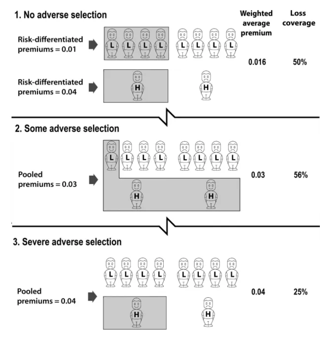
The argument can be illustrated with a toy example, in the same spirit as dice-rolling examples to illustrate probability laws. Consider a population of just ten risks (say lives), and three alternative scenarios for risk classification: risk-differentiated premiums, pooled premiums (with some adverse selection), and pooled premiums (with severe adverse selection). We assume that all losses and insurance cover are for unit amounts (this simplifies the discussion, but it is not necessary). We assume the probability of loss is unaffected by the purchase of insurance (i.e. no moral hazard). The three scenarios are represented in the three panels of Figure 1.
In Figure 1, each H represents one higher risk and each L represents one lower risk. The population has the typical predominance of lower risks: a lower risk-group of eight risks each with probability of loss 0.01, and a higher risk-group of two risks each with probability of loss 0.04. In each scenario, the shaded cover above some of the H and L denote the risks covered by insurance.
In Scenario 1, risk-differentiated premiums (actuarially fair premiums) are charged. The proportion of each risk-group which buys insurance under these conditions is 50%, in line with industry statistics for e.g. life insurance.1 The shading shows that a total of five risks are covered.
The weighted average of the premiums paid is (4 x 0.01 +1 x 0.04)/5 = 0.016. Since higher and lower risks are insured in the same proportions as they exist in the population, there is no adverse selection. The expected losses compensated by insurance for the whole population can be indexed by:
Loss coverage = Expected compensated losses Expected population losses =
4×0.01 + 1×0.04
8×0.01 + 2×0.04 = 50%. (1) In Scenario 2, in the middle panel of Figure 1, risk classification has been banned, and so insurers have to charge a common pooled premium to both higher and lower risks. Higher risks buy more insurance, and lower risks buy less. The weighted average premium
1
Some relevant industry statistics are as follows. The Life Insurance Market Research Organisation (LIMRA) states that 44% of US households have some individual life insurance (LIMRA (2013)). The US adult population (aged 18 years and over) at 1 July 2013 as estimated by the US Census Bureau was 244m; the American Council of Life Insurers states that 144m (59%) individual policies were in force in 2013 (ACLI, 2014, p72).
Figure 1: Three scenarios for risk classification (Adapted with permission from Thomas (2017)).
is (1 x 0.01 +2 x 0.04)/3 = 0.03. The shading shows that three risks (compared with five previously) are now covered.
Note that the weighted average premium is higher in Scenario 2, and the number of risks insured is smaller. These are the essential features of adverse selection, which Scenario 2 accurately and completely represents. But there is a surprise: despite the adverse selection in the second scenario, the expected losses compensated by insurance for the whole population are now larger. Visually, this is represented by the larger area of shading in Scenario 2. Arithmetically, the loss coverage is:
Loss coverage = 1×0.01 + 2×0.04
8×0.01 + 2×0.04 = 56%. (2)
We argue that Scenario 2, with a higher expected fraction of the populations losses compensated by insurance – higher loss coverage – is superior from a social viewpoint to Scenario 1. The superiority of Scenario 2 arises notdespite adverse selection, butbecause of adverse selection.
However, a ban on risk classification can also reduce loss coverage, if the adverse selection which the ban induces becomes too severe. This possibility is illustrated in Scenario 3, in the lower panel of Figure 1. Adverse selection has progressed to the point where only one higher risk, and no lower risks, buys insurance. Visually, the lower loss coverage is represented by the smaller area of shading in Scenario 3. Arithmetically, the loss coverage is:
Loss coverage = 1×0.04
8×0.01 + 2×0.04 = 25%. (3)
These scenarios suggest that banning risk classification can increase loss coverage if it induces the ‘right amount’ of adverse selection (Scenario 2), but reduce loss coverage if it generates ‘too much’ adverse selection (Scenario 3). Which of Scenario 2 or Scenario 3 actually prevails depends on the demand elasticities of higher and lower risks. Hence it is of interest to explore the demand elasticity conditions under which loss coverage is increased by a ban on risk classification.
3. Insurance Demand
In the toy example, the possibility of an increase in loss coverage when risk classifi-cation was banned depended on the fact that not all higher-risk individuals chose to buy insurance at an actuarially fair premium. This corresponds to the reality of voluntary in-surance markets (e.g. see the figures in Footnote 1). But it is not consistent with typical theories of insurance demand, which imply that all individuals will purchase full insurance if offered an actuarially fair premium (e.g. Mossin (1968)). This section presents a theory of insurance demand which accommodates the observable reality that not all individuals with the same probabilities of loss make the same insurance purchasing decision.
In Hao et al. (2016a), we assumed that some fixed proportion of individuals in each risk-group purchased insurance, consistent with the observation that in voluntary insur-ance markets, many individuals do not buy insurinsur-ance. Thus, the model of insurinsur-ance purchasing was at the level of the collective. In Hao et al. (2016b), we provided a micro-foundation for the collective model, based on personal utilities. We assumed that personal utilities within a risk-group are heterogeneous, so that different persons will make differ-ent decisions, when offered the same insurance premium. If the heterogeneity of utilities can be described in terms of a probability distribution, then the collective decision model of Hao et al. (2016a) can be recovered in terms of expected values.
This micro-foundation provides the ‘back-story’ for the proportional insurance de-mand functions which we use in Section 4 onwards. Because the ‘back-story’ is not the primary focus of this paper, the presentation here will be succinct. For a comprehensive account of the full probabilistic model underpinning this formulation, please refer to Hao et al. (2016b).
3.1 Micro-foundations: Heterogeneity in Individual Risk Preferences Consider an individual with an initial wealth W, who risks losing an amount of L with probabilityµ. Suppose wealth preferences are governed by the utility functionU(w), which is increasing in wealth w, i.e. U′(w) >0. (Individuals are typically also assumed to be risk-averse i.e. U′′(w) < 0, but our theory of insurance demand does not require that all individuals are risk-averse.)
Suppose that the individual is offered insurance against the full amount of loss L at premium rate π per unit of loss, i.e. for premiumπL. She will choose to buy insurance if π is low enough to satisfy:
U(W −πL)>(1−µ)U(W) +µ U(W −L). (4) In the above model, all individuals with the same probability of lossµmake the same purchasing decision, depending only on whether or not the offered premium rateπis small enough to satisfy Equation 4. In reality, not all individuals with the same probability of loss make the same purchasing decision (e.g. for life insurance, see the figures in footnote 1).
A possible explanation for this apparent inconsistency (see e.g. Finkelstein and Mc-Garry (2006); Cutler et al. (2008)) is that risk preferences are heterogeneous. That is, in a risk-group in which all individuals have the same risk µ, individuals may have different utility functions. Suppose for simplicity that utility functions belong to a family param-eterized by a positive real number γ. So a particular individual’s utility function can be denoted by Uγ(w).
Further suppose that, within the risk-group, γ is sampled randomly from some ran-dom variable Γ with distribution function FΓ(γ). So, a particular individual’s utility function, Uγ(w), is a random quantity. Any numerical quantity involving an individual’s
utility function is therefore a random variable, the randomness being inherited from the distribution FΓ(γ).
Now, a single individual in the risk-group will choose to buy insurance at premium rate π if and only if Equation 4 is satisfied for their particular utility functionUγ(w):
Uγ(W −πL)>(1−µ)Uγ(W) +µ Uγ(W −L). (5) Note that this behaviour is completely deterministic, assuming that individuals know their own preferences.
Since decisions based on Equation 5 do not depend on the origin and scale of a utility function, we will find it convenient to assume that all individuals have the same utility at the ‘end points’ W −Land W. The following standardisation is convenient: Uγ(W) = 1 and Uγ(W −L) = 0. Equation (5) then becomes:
Uγ(W −πL)>(1−µ). (6)
The utility at the fixed wealth (W −πL) is a random variable, that we denote by UΓ(W −πL), with a distribution function induced by the random variable Γ.
We now make the key assumption, that while individuals know their own utility function, this is unobservable to the insurer. Insurers can observe the probability of loss µ, and naturally know the offered premium rateπ, but within the risk-group the insurer can at most observe the proportion of individuals who choose to buy insurance. We call this a (proportional) demand function and define it as:
d(π) = P [UΓ(W −πL)>(1−µ)]. (7) Clearly, 0 ≤ d(π) ≤ 1, so d(π) is a valid probability. It is intuitively clear (and can be proved) that d(π) is non-increasing in π, so increasing the premium cannot increase demand for insurance.
Note that each individual’s decision is completely deterministic, given their knowledge of their own utility function; but to the insurer it appears stochastic, given what the insurer knows. In respect of any individual chosen randomly, define the function Qto be Q= 1 if they buy insurance or Q= 0 if they do not. To the individual concerned, Qis a deterministic function. To the insurer, Q is a Bernoulli random variable with parameter d(π).
As a concrete example, Result A.1 of Appendix A shows the iso-elastic demand func-tion obtained in the case of power utility funcfunc-tions parameterized by a random variable Γ with a specified distribution.
3.2 Aggregates: Proportional Demand and Demand Elasticities
The micro-foundations described above provide a possible mechanism by which aggre-gate demand for insurance is generated by the unobserved utility functions of individuals.
In the remainder of this paper, we work directly with the aggregate quantity, the propor-tional demand d(π) for insurance (0≤d(π)≤1).
We now define a related concept, the (point price) elasticity of insurance demand, as follows:
ǫ(π) =−∂ logd(π)
∂ logπ , or, equivalently: (8)
d(π) =τexp − Z π µ ǫ(s)dlogs , (9)
where the parameter τ =d(µ) is the fair-premium demand for insurance. The definition in Equation 9 has the benefit that we do not have to impose any regularity conditions, like continuity and differentiability, on the demand function d(π). We require only that the demand elasticity ǫ(π) in Equation 8 is non-negative, so that the demand d(π) in Equation 9 is non-increasing in premium π.
4. Equilibrium and loss coverage for two or more risk-groups
4.1 Framework for Insurance Risk Classification
In Section 3, we suggested a model for insurance demand from a group of individuals who all have the same probability of loss but who may have different risk preferences. We call such a group of individuals a risk-group. In this section, we extend the model to a population consisting of several risk-groups with different loss probabilities.
Suppose a population consists of ndistinct risk-groups with probabilities of loss given byµ1, µ2, . . . , µn. For convenience, we assume that 0< µ1 < µ2 < . . . < µn <1.
Suppose the proportion of the population belonging to risk-group i is pi, for i = 1,2, . . . , n. If we choose an individual at random from the population, their probability of loss is a random variable, which we denote by µ, and its distribution is given by P[µ=µi] =pi for i= 1,2, . . . , n.
Suppose insurers charge premiums π1, π2, . . . , πn for the risk-groups i = 1,2, . . . , n, respectively. Based on the model of Section 3, the demand for insurance within risk-group i is denoted bydi(πi), where 0≤di(πi)≤1 and di(πi) is non-increasing in πi.
Let the insurance purchasing decision of an individual chosen at random from the whole population be represented by the indicator random variable Q, taking the value of 1 if insurance is purchased; and 0 otherwise. Within risk-groupi,Qis a Bernoulli random variable defined as:
Then the expected demand for insurance across the the whole population, i.e. the expected proportion who buy insurance, is the unconditional expected value of Q:
E[Q] = n X i=1 E[Q|µ=µi] P[µ=µi] = n X i=1 di(πi)pi. (11)
Now suppose that the occurrence of a loss event for an individual chosen at random from the whole population is represented by the indicator random variable,X, taking the value of 1 if a loss event occurs; and 0 otherwise. Within risk-group i, X is a Bernoulli random variable defined as:
E[X |µ=µi] = P[X = 1|µ=µi] =µi (12) and the expected loss of an individual chosen at random from the population is the unconditional expected value of X:
E[X] = n X i=1 E[X |µ=µi] P[µ=µi] = n X i=1 µipi. (13)
Conditional on µ = µi, we assume that Q and X are independent. This ensures that there is no moral hazard; although the level of risk may influence the decision to buy insurance, mediated by di(πi), insured individuals in any risk-group have the same probability of loss as uninsured individuals. The expected insurance claim in respect of an individual chosen at random from the population is then:
E[QX] = n X i=1 E[QX |µ=µi] P[µ=µi], = n X i=1 E[Q|µ=µi] E[X |µ=µi] P[µ=µi], = n X i=1 di(πi)µipi. (14)
Next, define Π to be the premium paid by an individual chosen at random from the population. Then Π is a random variable. Since individuals who do not purchase insurance pay a premium of zero, we have Π =QΠ. Then within risk-group i:
E[ Π|µ=µi] = E[QΠ|µ=µi] = E[Q|µ=µi]πi =di(πi)πi (15) and the unconditional expected premium income is:
E[Π] = n X i=1 E[ Π|µ=µi] P[µ=µi] = n X i=1 di(πi)πipi. (16)
We call any vector of premiums (π1, π2, . . . , πn) charged by insurers a risk classification regime, and denote it by underlined characters such as π. The insurer’s expected profit under risk classification regime π, which we denote by ρ(π) is then :
ρ(π) = E[Π]−E[QX] = n X i=1 di(πi)πipi− n X i=1 di(πi)µipi. (17)
Equilibrium in the insurance market is defined by ρ(π) = 0. We assume that competition between insurers compels all insurers to use the same risk classification regime, which must be an equilibrium regime. Depending on applicable regulation, two polar cases of equilibrium risk classification regimes are as follows:
Full risk classification, under which πi = µi. Here, the insurer uses the maximum possible degree of underwriting. We denote this regime by µ.
No risk classification, or risk pooling, under which all πi =π, a constant. Here, the insurer uses the minimum possible degree of underwriting.
By considering the insurer’s profit under risk pooling withπ =µ1 and π =µn, it is clear that there must be at least one risk pooling regime which leads to equilibrium.2
4.2 Loss coverage
We define loss coverage under a risk classification π that leads to equilibrium as the expected losses across the whole population that are compensated by insurance, i.e. E[QX] as defined in Equation 17. That is:
Loss coverage: LC(π) = E[QX], (18)
where ρ(π) = 0.
For comparison purposes we use loss coverage under full risk classification regime as a reference level, and hence define the loss coverage ratio as follows:
Loss coverage ratio: C = LC(π)
LC(µ). (19)
5. Impact of Demand Elasticities on Loss Coverage 2
In general, there may be more than one, and the results in this paper allow for this possibility. But such multiple solutions do not arise for typical demand functions and elasticities. For more details see Hao et al. (2016b) and Appendix B of Thomas (2017).
In this section we investigate the impact of demand elasticities for higher and lower risks on loss coverage ratio. For ease of exposition we start with iso-elastic demand where all risk-groups have the same elasticity λ, and use this as a stepping stone to prove successively more general results.
5.1 Same Iso-elastic Demand Elasticity for all Risk-groups
Suppose the elasticity of demand is the same constant for all individuals, irrespective of their risks and of the premium charged, i.e. insurance demand is iso-elastic. So:
ǫi(π) = λ (a positive constant), for i= 1,2, . . . , n. (20) The resulting demand function found from Equation 9 is:
di(π) = τi µi
π λ
, i= 1,2, . . . , n. (21)
Based on this demand, the equilibrium condition under risk pooling, i.e. ρ(π0) = 0, gives: n X i=1 piτi µi π0 λ (π0−µi) = 0, or, equivalently: (22) n X i=1 αi µi π0 λ = n X i=1 αi µi π0 λ+1 , where αi = piτi Pn i=1piτi for i= 1,2, . . . , n, (23) and the unique pooled equilibrium premium, π0, is given by:
π0 = Pn i=1αiµλi+1 Pn i=1αiµλi (24) To facilitate mathematical proofs, it is helpful to re-frame Equation 23 as follows. Consider a random variable, V, taking values vi = πµ0i with probabilities αi for i = 1,2, . . . , n. Then Equation 23 says that under equilibrium, the random variableV satisfies:
E Vλ
= E Vλ+1
. (25)
The loss coverage ratio, as defined in Equation 19, comparing loss coverage under pooled premiums to that under risk-differentiated premiums, can be re-framed as:
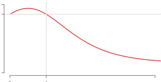
C = LC(π0) LC(µ) = Pn i=1αi µi π0 λ µi Pn i=1αiµi = Pn i=1αi µi π0 λ+1 Pn i=1αi µi π0 = E Vλ+1 E [V] = E Vλ E [V] . (26) Figure 2 shows the plot of loss coverage ratio as a function of demand elasticityλ, for the risks (µ1, µ2) = (0.01,0.04) and (α1, α2) = (0.8,0.2). We can see that loss coverage under pooling is higher than under risk-differentiated premiums if demand elasticity is less than 1, and vice versa. The pattern shown in Figure 2 is formally stated in the following result:
λ (Demand elasticity) Loss co v erage ratio 0 1 0.4 1
Figure 2: Loss coverage ratio as a function of demand elasticity for iso-elastic demand.
Result 5.1. Suppose there are n risk-groups with risks µ1 < µ2 <· · ·< µn and the same
iso-elastic demand elasticity λ. Then λ⋚1⇒C R1.
This result generalises a result proved for only two risk-groups in Hao et al. (2016a). A proof is given in Appendix B.
5.2 Different Iso-elastic Demand Elasticities for Different Risk-groups The assumption of constant iso-elastic demand elasticity for all individuals, although mathematically tractable, can be criticised as unrealistic. For most goods and services, we expect demand elasticity to rise with price, because of the income effect on demand: at higher prices, the good forms a larger part of the consumer’s total budget constraint, and so the effect of a small percentage change in its price might be larger. For insurance this suggests that demand elasticity for higher risks (who are typically charged higher prices) might be higher. So we next consider iso-elastic demand functions with different demand elasticities for different risk-groups, i.e.:
ǫi(π) =λi fori= 1,2, . . . , n; (27)
formu-lation, the equilibrium condition under risk pooling, i.e. ρ(π0) = 0, gives: n X i=1 piτi µi π0 λi (π0−µi) = 0, or, equivalently: (28) n X i=1 αi µi π0 λi = n X i=1 αi µi π0 λi+1 . (29)
As in Section 5.1, we define a random variable V taking values vi = πµ0i with proba-bilities αi for i= 1,2, . . . , n. Now, define a function f(v), such that:
f(vi) =λi, for i= 1,2, . . . , n. (30)
Then the equilibrium condition, in Equation 29, can be re-framed as: E
Vf(V) = E
Vf(V)+1
. (31)
Under this setting, we have the following result:
Result 5.2. Suppose there are n risk-groups with risks µ1 < µ2 < · · · < µn with
iso-elastic demand iso-elasticities λ1, λ2, . . . , λn respectively. Defineλlo = maxv≤1f(v) andλhi = minv>1f(v). Then λlo<1 and λhi ≥λlo ⇒C ≥1.
To understand this result, note that under pooled equilibrium, λlo is the maximum of the demand elasticities of all those lower risk-groups who pay more premium,π0, than their actuarially fair risk µ. So, λlo < 1 signifies that, for these lower risk-groups, their iso-elastic demand elasticities should be less than 1, which is consistent with empirical evidence in many markets (as discussed in Section 6 of this paper).
On the other hand, λhi, is the minimum of the demand elasticities of all those higher risk-groups who pay less premium, π0, than their actuarially fair risk, µ. The interpreta-tion of the second condiinterpreta-tion, λhi ≥ λlo, is that for these higher risk-groups, the demand elasticities should be larger than those of all the lower risk-groups, which is consistent with what we expect from the income effect on demand.
In summary, as long as the iso-elastic demand elasticities of the different risk-groups satisfy the two conditions: λlo <1 andλhi ≥λlo, the loss coverage under pooling is higher than under full risk classification.
The following special cases of Result 5.2 are worth noting:
1. If the iso-elastic demand elasticities are the same for all risk-groups, i.e. λi =λ for i = 1,2, . . . , n, then by definition λlo = λhi = λ, and so λlo = λ < 1 gives C ≥ 1, which corresponds to Result 5.1.
2. For the special case of: 0 < λ1 ≤ λ2 ≤ · · · ≤ λn < 1, the two conditions, λlo < 1 and λhi ≥λlo, are trivially satisfied and hence in this case: C ≥1.
3. For the case of two risk-groups, λlo = λ1 and λhi = λ2, and the conditions on the demand elasticities translate to λ1 <1 and λ2 ≥λ1.
The two risk-groups case is illustrated in Figure 3, where (µ1, µ2) = (0.1,0.4) and (α1, α2) = (0.8,0.2). The two axes represents λ1 and λ2. The figure demarcates the region of C >1 (shaded green) from the region of C <1 (shaded pink) by the boundary curve C = 1 (in red).
The conditions on λ1 and λ2 say that in the region above the λ1 = λ2 diagonal and λ1 < 1, demarcated by the green dashed borders, loss coverage under pooling is always higher than that under full risk classification. This is true irrespective of the relative sizes and relative risks of the higher and lower risk populations.
Figure 3 highlights another important point: that Result 5.2 focuses only on loss coverage inside the region demarcated by green dashes. Outside this region, loss coverage under pooling can be higher or lower than under full risk-classification (higher in the green segments to the right of the dashed green lines; lower throughout the red area towards the right). The position of theC = 1 curve which demarcates the red and green areas changes slightly with relative population sizes and relative risks. The region demarcated by green dashes is the only region for which we can obtain a universal result (i.e. one which holds independent of relative sizes and risks of higher and lower risk populations). Fortuitously, empirical evidence and economic rationale imply that realistic values of (λ1, λ2) may often fall within this region.
A proof of Result 5.2 is given in Appendix C. 5.3 General Demand Elasticity Functions
So far, we have only considered constant demand elasticities (as a function of pre-mium), either for all individuals in the population, or for all individuals belonging to a particular risk-group. However, it can be argued that demand elasticities should actually be increasing functions of premium (instead of being a constant), to reflect the income ef-fect on demand; the argument being that at higher prices, insurance forms a larger part of the consumer’s total budget constraint. In this section, we generalise our analysis to allow for different demand elasticity functions, ǫi(π), for different risk-groups i= 1,2, . . . , n.
Using Equation 9, the proportional demand for insurance, for risk-group i, is: di(π) = τiexp − Z π µi ǫi(s)dlogs , for i= 1,2, . . . , n. (32)
λ1 λ2 0.0 0.5 1.0 1.5 0.0 0.5 1.0 1.5 C>1 C<1 C=1
Figure 3: Curve demarcating the regions where loss coverage ratio is greater than and less than 1 when (µ1, µ2) = (0.1,0.4) and (α1, α2) = (0.8,0.2).
Under this formulation, the equilibrium condition under risk pooling, i.e. ρ(π0) = 0, gives: n X i=1 piτiexp − Z π0 µi ǫi(s)dlogs (π0−µi) = 0, or, equivalently: (33) n X i=1 αiexp Z µi π0 ǫi(s)dlogs (π0−µi) = 0; (34)
in which the term:
Z µi
π0
ǫi(s)dlogs, (35)
can be interpreted using the concept of arc elasticity of demand, denoted by ηi(a, b) and defined in Vazquez (1995) as follows:
ηi(a, b) = Rb a ǫi(s)dlogs Rb a dlogs . (36)
Arc elasticity, ηi(a, b), can be interpreted as the average value of (point) elasticity of demand for risk-group i, ǫi(s), over the price logarithmic arc from price a to price b. So in our case, we can define:
λi =ηi(π0, µi) = Rµi π0 ǫi(s)dlogs Rµi π0 dlogs , for i= 1,2, . . . , n. (37) Equation 34 can then be rewritten using arc elasticities as follows:
n X i=1 αiexp λi Z µi π0 dlogs (π0 −µi) = 0, or, equivalently: (38) n X i=1 αi µi π0 λi (π0−µi) = 0 (39)
Note that Equation 39 is identical in form to Equation 29, but with the relevant arc elasticities substituted for point elasticities.
The general result, as stated below, then follows directly from Result 5.2:
Result 5.3. Suppose there are n risk groups with risks µ1 < µ2 <· · ·< µn with demand
elasticitiesǫ1(π), ǫ2(π), . . . , ǫn(π), such thatλ1, λ2, . . . , λnare the respective arc elasticities under pooled equilibrium. Define λlo = maxv≤1f(v) and λhi = minv>1f(v). Then λlo < 1 and λhi ≥λlo ⇒C≥1.
In other words, under pooled equilibrium, as long as the arc elasticities of lower risk-groups (paying more than their fair actuarial premium) do not exceed 1 and the arc elasticities of the higher risk-groups (paying less than their fair actuarial premium) in all cases exceed those of the lower risk-groups, then loss coverage under pooling is higher than under full risk classification.
For the special case ofǫi(π) being non-decreasing functions of premiumπand bounded above by 1, where ǫ1(π)≤ǫ2(π)≤ · · · ≤ ǫn(π) the required conditions for Result 5.3 are automatically satisfied. This is because the arc elasticities of demand, being an average of the underlying point elasticities, satisfy: 0 < λ1 ≤ λ2 ≤ · · · ≤ λn < 1, which then implies that λlo <1 and λhi ≥λlo and thusC ≥1.
6. Discussion
The results obtained in Section 5 suggest that loss coverage will be higher under pooling than under full risk classification, if
1. elasticity (or arc elasticity, if elasticity is not constant) is less than 1 for all lower risk-groups; and
2. elasticity (or arc elasticity, if elasticity is not constant) for all higher risk-groups exceeds that for all lower risk-groups,
where arc elasticities are logarithmic averages of demand elasticities over the arc, from true risk price to the equilibrium pooled price.
Are these conditions likely to be satisfied in the real world?
For the first condition, Table 1 shows some relevant empirical estimates for insurance demand elasticities.3 It can be seen that most estimates are of magnitude significantly less than 1. Whilst the various contexts in which these estimates were made may not correspond closely to the set-up in this paper, the figures are at least suggestive of the possibility that the first condition may often be satisfied.
Table 1: Estimates of demand elasticity for various insurance markets Market & country Demand elasticities Authors
Term life insurance, USA -0.66 Viswanathan et al. (2006) Yearly renewable term life, USA -0.4 to -0.5 Pauly et al. (2003) Whole life insurance, USA -0.71 to -0.92 Babbel (1985) Health insurance, USA 0 to -0.2 Chernew et al. (1997),
Blumberg et al. (2001), Buchmueller and Ohri (2006) Health insurance, Australia -0.35 to -0.50 Butler (1999)
Farm crop insurance, USA -0.32 to -0.73 Goodwin (1993)
For the second condition, we know of no empirical evidence that insurance demand elasticities are higher (or lower) for higher risks. However, as noted earlier in the paper, this condition may be plausible in that it is consistent with the income effect on demand.
7. Conclusions
Loss coverage is defined as the expected population losses compensated by insurance at market equilibrium. We suggest that if the social purpose of insurance is to compensate the population’s losses, loss coverage may be an intuitively appealing metric for evaluation of different risk classification schemes.
When risk classification is banned, so that insurers have to pool all risks at a single price, this can lead to adverse selection. Adverse selection is associated with a fall in the number of insured individuals compared with that obtained under full risk classification.
3
Demand elasticity is defined as a positive constant in this paper for convenience, but estimates in empirical papers are generally given with the negative sign, so Table 1 quotes them in that form.
However, adverse selection is also associated with a shift in coverage towards higher risks. If the shift is large enough, it can more than offset the fall in numbers insured, so that loss coverage is increased. We suggest that from a social perspective, this possibility might be seen as a good outcome from adverse selection.
Whether loss coverage is in fact increased when all risks are pooled depends on the response of higher and lower risks to changes in the prices they face, that is the demand elasticities of higher and lower risks.
This paper has stated demand elasticity conditions which ensure that loss coverage will be higher under pooling than under fully risk-differentiated premiums. The condi-tions were stated for successively more general contexts: first, for iso-elastic demand with a single elasticity parameter; second, for iso-elastic demand with different elasticity pa-rameters for different risk-groups; and third, for any downward-sloping demand functions (including different ones for different risk-groups). The demand elasticities required for loss coverage to be higher under pooling seem realistic for some insurance markets.
Acknowledgements
MingJie Hao thanks Radfall Charitable Trust for research funding. References
D. Babbel. The price elasticity of demand for whole life insurance. Journal of Finance, 40(1): 225–239, 1985.
L. Blumberg, L. Nichold, and J. Banthin. Worker decisions to purchase health insurance. International Journal of Health Care Finance and Economics, 1:305–325, 2001.
T.C. Buchmueller and S. Ohri. Health insurance take-up by the near-elderly. Health Services Research, 41:2054–2073, 2006.
J.R. Butler. Estimating elasticities of demand for private health insurance in australia. Working Paper No. 43. National Centre for Epidemiology and Population Health ,Australian National University, Canberra, 1999.
M. Chernew, K. Frick, and C. McLaughlin. The demand for health insurance coverage by low-income workers: Can reduced premiums achieve full coverage? Health Services Research, 32: 453–470, 1997.
D.M. Cutler, A. Finkelstein, and K. McGarry. Preference heterogeneity and insurance markets: Explaining a puzzle of insurance. American Economic Review, 98:157–162, 2008.
G. Dionne and C.G. Rothschild. Economic effects of risk classification bans. Geneva Risk and Insurance Review, 39:184–221, 2014.
L. Einav and A. Finkelstein. Selection in insurance markets: theory and empirics in pictures. Journal of Economic Perspectives, 25:115–138, 2011.
A. Finkelstein and K. McGarry. Multiple dimensions of private information: evidence from the long-term care insurance market. American Economic Review, 96:938–958, 2006.
B.K. Goodwin. An empirical analysis of the demand for multiple peril crop insurance. American Journal of Agricultural Economics, 75(2):424–434, 1993.
M. Hao, A.S. Macdonald, P. Tapadar, and R.G. Thomas. Insurance loss coverage under restricted risk classification: The case of iso-elastic demand. ASTIN Bulletin, 2016a. http://dx.doi.org/10.1017/asb.2016.6.
M. Hao, A.S. Macdonald, P. Tapadar, and R.G. Thomas. Insurance loss coverage and social welfare. http://kar.kent.ac.uk/54235, 2016b.
M. Hoy. Risk classification and social welfare. Geneva Papers on Risk and Insurance, 31:245–269, 2006.
J. Mossin. Aspects of rational insurance purchasing. Journal of Political Economy, 76:553–568, 1968.
M.V. Pauly, K.H. Withers, K.S. Viswanathan, J. Lemaire, J.C. Hershey, K. Armstrong, and D.A. Asch. Price elasticity of demand for term life insurance and adverse selection. NBER Working Paper (9925), 2003.
R.G. Thomas. Loss coverage as a public policy objective for risk classification schemes. Journal of Risk and Insurance, 75:997–1018, 2008.
R.G. Thomas. Demand elasticity, risk classification and loss coverage: when can community rating work? ASTIN Bulletin, 39:403–428, 2009.
R.G. Thomas. Loss Coverage: Why Insurance Works Better With Some Adverse Selection. Cambridge University Press, 2017.
A. Vazquez. A note on arc elasticity of demand. Estudios Economicos, 10(2):221–228, 1995. K.S. Viswanathan, J. Lemaire, K. K. Withers, K. Armstrong, A. Baumritter, J. Hershey,
M. Pauly, and D.A. Asch. Adverse selection in term life insurance purchasing due to the brca 1/2 genetic test and elastic demand. Journal of Risk and Insurance, 74:65–86, 2006.
Appendices
A. Microfoundation of Insurance Demand
Suppose, for simplicityW =L= 1, and individuals’ risk preferences are driven by a power utility function:
Uγ(w) =wγ, (40)
so that Uγ(0) = 0 andUγ(1) = 1. This particular form of utility function leads to:
relative risk aversion coefficient: −wU ′′ γ(w) U′
γ(w)
= 1−γ. (41)
So the heterogeneity in preferences between individuals can be modelled through the randomness of the risk aversion parameterγ. As outlined in Section 3, we define a positive random variable Γ, and individual risk preferences γ are then instances drawn from the distribution of Γ.
Inserting this utility function into Equation 7, the demand for insurance at a given premium π is then:
d(π) = P [UΓ(1−π)>1−µ], (42) = P
(1−π)Γ>1−µ
, (43)
= P [Γ log(1−π)>log(1−µ)], as log is monotonic, (44) = P Γ< log(1−µ) log(1−π) , as log(1−π)<0. (45) So, given an observed (proportional) insurance demand function, which is non-increasing in premium, π, the underlying random variable Γ has the following distribution function:
FΓ(γ) = P [Γ< γ] =d(1−(1−µ)1/γ). (46)
Since 1−(1−µ)1/γ ≈µ/γ for smallµ, we might in some circumstances approximate equation (46) by the simpler: FΓ(γ) = P [Γ< γ] =d µ γ . (47)
Note thatFΓ(γ) is a non-decreasing function and lies between 0 and 1.
Of course, forFΓto be a valid distribution function, we would also require limγ→0FΓ(γ) = 0 and limγ→∞FΓ(γ) = 1, or equivalently, limπ→∞d(π) = 0 and limπ→0d(π) = 1, which appear to be reasonable assumptions. However, empirical observations are unlikely to be available for these extreme cases, so it is only possible to model insurance purchasing behaviour over the range of premiums observed in the market, with appropriate extrapolations at the limiting extremes.
Result A.1. Given an observed proportional insurance demand,d(π), which is a valid probability
and non-increasing in π, heterogeneity of risk preferences driven by the power utility function
and characterised by the random parameter Γ with the distribution function given by Equation
46 produces the observed demand for insurance for small premiums.
We illustrate the above result using iso-elastic demand: Suppose Γ has the following distri-bution: FΓ(γ) = P [Γ≤γ] = 0 ifγ <0 τ γλ if 0≤γ ≤(1/τ)1/λ 1 ifγ >(1/τ)1/λ, (48)
where τ and λ are positive parameters. Note that τ = λ= 1 leads to a uniform distribution. λ controls the shape of the distribution function and τ controls the range over which Γ takes its values. Then the demand for insurance, as given in Equation (45), takes the form (under certain parameter constraints):
d(π) =τµ π
λ
, (subject to a cap of 1) (49) which corresponds to iso-elastic demand, the constant demand elasticity being:
ǫ(π) =−∂log(d(π))
∂logπ =λ. (50) The parameterτ can also be interpreted as thefair-premium demand, that is the demand when an actuarially fair premium is charged.
B. Equal Iso-elastic Demand Elasticities
Using the formulation of Section 5.1, we prove the following result.
Result B.1. Let V be a positive random variable and λ be a positive constant, such that
E Vλ = E Vλ+1 . Then: λ⋚1⇒EhVλiRE [V]. (51)
Proof. Case: λ= 1: It follows directly from the definition.
Case: 0< λ <1: Holder’s inequality states that, if 1 < p, q < ∞ where 1/p+ 1/q = 1, for
positive random variablesX, Y with E[Xp],E[Yq]<∞:
(E [Xp])1/p(E [Yq])1/q ≥E[XY]. (52)
Setting 1/p=λ, 1/q = 1−λ,X=Vλ2
and Y =V1−λ2
, Holder’s inequality gives:
EhVλ2 1λ iλ EhV(1−λ2) 1 1−λ i1−λ ≥EhVλ2V1−λ2i, (53) ⇒EhVλiλEhVλ+1i1−λ ≥E [V], (54) ⇒EhVλi≥E [V], since EhVλi= EhVλ+1i. (55)
Case: λ >1: Young’s inequality states that, fora, b≥0 and p, q >0 such that 1/p+ 1/q= 1:
ab≤ a p p + bq q . (56) Settingp=λ,q= λ−λ1,a=Vλ1 and b=Vλ− 1
λ, Young’s inequality gives:
Vλ1Vλ− 1 λ ≤ 1 λV 1 λλ+λ−1 λ V (λ−1 λ) λ λ −1, (57) ⇒Vλ≤ 1 λV + λ−1 λ V λ+1, (58) ⇒EhVλi≤ 1 λE [V] + λ−1 λ E h Vλ+1i, (59) ⇒EhVλi≤E [V], since EhVλi= EhVλ+1i. (60)
Result 5.1 follows directly from Result B.1 by noting that: C= E Vλ
C. Different Iso-elastic Demand Elasticities
Using the formulation of Section 5.2, we prove the following result:
Result C.1. Let V be a positive random variable and f(v) be a positive function, such that
E Vf(V)
= E
Vf(V)+1
. Define λlo= maxv≤1f(v) and λhi= minv>1f(v). Then:
λlo<1 and λhi≥λlo⇒E h
Vf(V)i≥E [V]. (61)
Proof. Holder’s inequality states that, if 1< p, q <∞ where 1/p+ 1/q = 1, for positive random
variables X, Y with E[Xp],E[Yq]<∞:
(E [Xp])1/p(E [Yq])1/q ≥E[XY]. (62) For anyλ, such that 0< λ <1, set 1/p=λ, 1/q = 1−λ,X =Vλ f(V) and Y =V(1−λ)(f(V)+1), Holder’s inequality gives:
EhVf(V)iλEhVf(V)+1i1−λ ≥EhVλ f(V)V(1−λ)(f(V)+1)i, (63)
⇒EhVf(V)i≥EhVf(V)+1−λi, since EhVf(V)i= EhVf(V)+1i. (64) The relationship in Equation 64 holds for any positive λ <1. Now, set λ=λlo <1.
Case V <1: λlo= max v≤1 f(v)⇒f(V)≤λlo=λ⇒f(V) + 1−λ≤1⇒V f(V)+1−λ ≥V. (65) Case V = 1: Vf(V)+1−λ =V. (66) Case V >1: λhi= min v>1 f(v)⇒f(V)≥λhi≥λlo=λ⇒f(V) + 1−λ≥1⇒V f(V)+1−λ ≥V. (67)
Hence,Vf(V)+1−λ ≥V for all cases, which implies
EhVf(V)+1−λi≥E [V]. (68) Combining Equations 64 and 68, we have:
EhVf(V)i≥E [V]. (69)
Result 5.2 follows directly from Result C.1 by noting that the loss coverage ratio in this case is: C= E
Vf(V)