Regularization Methods for Predicting an Ordinal Response using Longitudinal High-dimensional Genomic Data

(1)

Virginia Commonwealth University

VCU Scholars Compass

Theses and Dissertations Graduate School

2013

Regularization Methods for Predicting an Ordinal

Response using Longitudinal High-dimensional

Genomic Data

Jiayi Hou

Virginia Commonwealth University

Follow this and additional works at:http://scholarscompass.vcu.edu/etd

Part of theBiostatistics Commons

This Dissertation is brought to you for free and open access by the Graduate School at VCU Scholars Compass. It has been accepted for inclusion in Theses and Dissertations by an authorized administrator of VCU Scholars Compass. For more information, please [email protected]. Downloaded from

(2)

c

(3)

REGULARIZATION METHODS FOR PREDICTING AN ORDINAL RESPONSE USING LONGITUDINAL HIGH-DIMENSIONAL GENOMIC DATA

A dissertation submitted in partial fulfillment of the requirements for the degree of Doctor of Philosophy at Virginia Commonwealth University

By Jiayi Hou

B.S. Mathematics, Sichuan University, 2008

Advisor: Kellie J. Archer

Associate Professor, Department of Biostatistics

Director, VCU Massey Cancer Center Biostatistics Shared Resource

Virginia Commonwealth University Richmond, Virginia

(4)

Acknowledgement

I own my sincere thanks to countless people who have helped, supported, encouraged me during my long Ph.D journey. Without your help, this thesis would not be possible. First and foremost, I must thank my thesis advisor Dr. Kellie Archer for the generous support she gave to help pave the path to achievement. Dr.Archer has inspired me to devote to statistical learning area by her enthusiasm, vision and determination. Learning from Dr. Archer has been the greatest pleasure and will be the lifetime treasure.

Thank you to the rest of my thesis committee: Dr. Chris Gennings, Dr. Robert Johnson who are experts in the fields of biostatistics; Dr. Sam Chen, who has tremendous research experience in genetics and genomics; and Dr. Juan Lu, who contributes enormously to the epidemiology area. Your constructive feedback, rich support and kind encouragement help me grow both as a researcher and as a person. I truly appreciate the time, effort and energy you dedicated to help make this happen. Many other great supervisors I got to know through various projects and positions have taught me a lot. Thank you to Dr. Mark Reimers for introducing me to the field of bioinformatics and offering me the rigorous training. Thank you to Dr. Charlie Kish and Dr. Carol Summitt for providing a unique opportunity to gain real industrial experience and broadening the areas where my knowledge can be applied. Thank you to Dr. Phillip Yates, Dr. Max Kuhn and other team members at Pfizer Inc for offering me an enjoyable, memorable and cool summer in Connecticut.

(5)

Reese, Chunfeng Ren, Qing Zhou, Yan Jin who grow, laugh, gossip and enjoy graduate school with me. There were other people in the department who provided generous support and helped me get through school: Yvonne Hargrove, Gayle Spivery, Helen Wang, Brian Bush, Russ Boyle, Dr. Donna McClish, Dr. Roy Sabo, Dr. Jessica Ketchum, Dr. Guimin Gao and Dr. Shumei Sun, I owe you a great debt of gratitude. I am grateful to all my other friends in Richmond, VA for your accompaniment, tolerance and encouragement which makes the journey wonderful.

Finally, I owe everything to my parents and family members who unconditionally support me to pursue my dream.

(6)

Table of Contents

Page

Table of Contents iii

List of Figures ix

List of Tables xii

Abstract xx

1 Introduction to Ordinal Model 1

1.1 Ordinal Responses . . . 2

1.2 Model Framework for Ordinal Responses . . . 3

1.2.1 Cumulative Logit Model . . . 5

1.2.2 Adjacent Categories Model . . . 6

1.2.3 Continuation Ratio Model . . . 8

1.3 Estimation of the Coefficients . . . 10

1.3.1 Maximum Likelihood Estimate . . . 10

1.3.2 Optimization Technique . . . 11

1.3.3 Software Implementation . . . 13

1.4 NIMH Schizophrenia Example . . . 14

(7)

2.1 Regularization Methods for Continuous Response . . . 21

2.1.1 LASSO . . . 24

2.1.2 Forward Stagewise Method . . . 26

2.1.3 LAR . . . 27

2.2 Regularization Methods for Dichotomous Responses . . . 28

2.2.1 LASSO for Logistic Regression . . . 29

2.2.2 Forward Stagewise for Logistic Regression . . . 30

2.3 Coordinate Descent for LASSO Regularization Paths . . . 32

2.4 Some Discussion . . . 35

3 Statistical Models for Longitudinal Data 37 3.1 Linear Mixed Model . . . 40

3.1.1 Linear Regression Model . . . 40

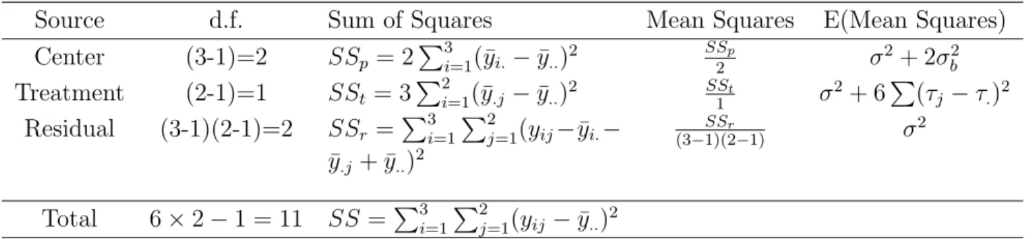
3.1.2 ANOVA and MANOVA Approaches for Repeated Measurement . . . 41

3.1.3 Linear Mixed Model . . . 47

3.1.4 Estimating Parameters for a Linear Mixed Model . . . 55

3.2 Nonlinear Mixed Model . . . 66

3.2.1 The Model Framework . . . 66

3.2.2 The Marginal Likelihood and its Approximation . . . 67

3.2.3 Estimating of the Parameters . . . 71

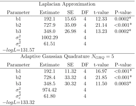
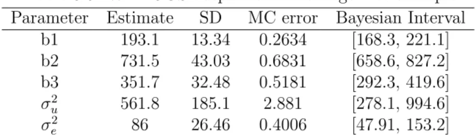
3.2.4 Orange Tree Example . . . 72

3.3 Generalized Linear Model . . . 79

3.3.1 Generalized Linear Model Framework . . . 79

(8)

3.3.3 Maximum Likelihood Estimates for GLM . . . 83

3.3.4 Quasi-Likelihood Estimates for GLM . . . 84

3.4 Generalized Linear Mixed Model . . . 87

3.4.1 Generalized Equation Estimation for Marginal Model . . . 87

3.4.2 Penalized Quasi-likelihood for GLMM . . . 89

4 Random Coefficient Model with Ordinal Response 94 4.1 Random Coefficient Model with Ordinal Response . . . 95

4.2 The Marginal Likelihood and its Approximation . . . 97

4.3 Estimating Model Parameters . . . 105

4.4 Estimating the Random Effects . . . 108

4.5 NIMH Schizophrenia Example Revisited . . . 109

4.6 Health Services Research Example . . . 122

5 Penalized Model for Traditional Longitudinal High-dimensional Data with an Ordinal Response 127 5.1 Review of Forward Stagewise Method . . . 128

5.2 Regularization Method for High-dimensional Data with Ordinal Response . . 131

5.3 Regularization Method for Longitudinal High-dimensional Data with an Or-dinal Response . . . 137

5.4 Model Assessment and Selection . . . 143

5.5 Software Implementation . . . 147

5.6 Simulations to Evaluate the Proposed Model . . . 166

(9)

5.6.2 Simulation for Longitudinal High-dimensional Data . . . 167

5.7 Some Discussion . . . 168

6 Application of Proposed Methodology 172 6.1 Application to the Smoking Study . . . 173

6.2 Application to the Glue Grant Study . . . 179

6.2.1 Marshall score for the renal system . . . 182

6.2.2 Marshall score for the central nervous system . . . 190

6.2.3 Aggregated Marshall score . . . 196

6.3 Discussion . . . 200

7 Conclusions and Future Work 203 7.1 Conclusions . . . 203

7.2 Future Work . . . 206

7.2.1 Variable Selection using LAR type Algorithm . . . 206

7.2.2 Variable Selection with Consideration of the Correlations between Fea-tures . . . 208

7.2.3 Application to Other Genomic and Medical Data . . . 210

Bibliography 213 Appendices 223 A NIMH Schizophrenia Data Code 224 A.1 R code for NIMH Schizophrenia Data . . . 224

(10)

A.3 SAS code for NIMH Schizophrenia Data . . . 228

B Orange Tree Example Code 230 B.1 R code for Orange Tree Example . . . 230

B.2 R code for Orange Tree Example using lme4 package . . . 233

B.3 SAS code Orange Tree Example . . . 234

B.4 WinBUGS code for Orange Tree Example . . . 235

C NIMH Schizophrenia Longitudinal Data Code 237 C.1 R code for NIMH Schizophrenia Longitudinal Data . . . 237

C.2 SAS code for NIMH Schizophrenia Longitudinal Data . . . 237

C.3 R code for NIMH Schizophrenia Longitudinal Data using ordinalpacakge . 241 D NIMH Schizophrenia Longitudinal Data Additional Results 242 D.1 Random Coefficient Model with Adjacent Categories Logit . . . 242

D.2 Random Coefficient Model with Backward Continuation Ratio . . . 248

D.3 Random Coefficient Model with Forward Continuation Ratio . . . 254

E Health Service Research Example Code 260 E.1 R code for Health Service Research Example . . . 260

E.2 SAS code for Health Service Research Example . . . 260

F Health Service Research Example Additional Results 262 F.1 Health Service Research Example output: Random Intercept Model with Adjacent-Category Logit . . . 262

(11)

F.3 Random Intercept Model with Forward Continuation Ratio Logit . . . 265

G GSE10006 Smoking Study Additional Results 267 H Glue Grant Burn Injury Study Example Additional Results 269 I R code for R package ordinalmixed with Applications 277 I.1 Source Code . . . 277

I.2 Application to NIMH Schizophrenia Longitudinal Data . . . 305

I.3 Application to Health Service Research Example . . . 306

I.4 Application to GSE10006 Smoking Study . . . 307

I.5 Application to Glue Grant Burn Injury Study . . . 310

I.6 High-dimensional Data Simulation . . . 317

(12)

List of Figures

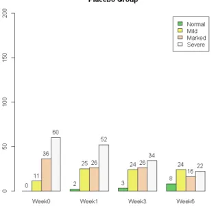
2.1 Estimation picture for the LASSO . . . 25 2.2 Least square projection in linear regression model . . . 27 3.1 Orange Tree Growth Curves . . . 72 4.1 Summary of IMPS score (Normal, Mild, Marked, Severe) by Time in the

Placebo Group . . . 110 4.2 Summary of IMPS score (Normal, Mild, Marked, Severe) by Time in the

Intervention Group . . . 111 4.3 Summary of Housing Status by Time in Group with Section 8 Certificates . 124 4.4 Summary of Housing Status by Time in Group without Section 8 Certificates 124 5.1 Flowchart for function FSPenFixed in R package ordinalmixed. The blue

circle represents input/output and the cyan rectangle represents an R func-tion. The FSPenFixed function first calls function forward.stagewise.cum

to perform steps 1,2 and 3 described in GMIFS for ordinal response with high-dimensional data. Those results get passed to additional functions (output.CumFS, steps, logLL) to perform step 4. By using ˆα and ˆβbiased from the optimal

parsimonious ordinal model, function Predict calculates the predicted ordi-nal response where the prediction error can be estimated by comparing it with the true ordinal response. . . 164

(13)

5.2 Flowchart for function FSPenFixed and ordinal.mixed.model in R pack-age ordinalmixed. The blue circle represents input/output and the cyan rectangle represents an R function. Function FSPenMixed consists of two parts: the GMIFS part and the ordinal random coefficient/intercept model part. The ordinal random coefficient/intercept model is fitted by function

ordinal.mixed.model, which is primarily shown in this flowchart. The GMIFS part is the same as that in function FSPenFixed where it first calls func-tion forward.stagewise.cum to perform steps 1, 2, 3 and 4 described in GMIFS for modeling a longitudinal ordinal response in the presence of high-dimensional data. Those results get passed to additional functions (output.CumFS, steps, logLL) to update the intercept estimates ˆα and decide the optimal set of features with nonzero coefficient estimates. The corresponding results get passed to functionordinal.mixed.model where a penalized ordinal coef-ficient/intercept model is fitted. This function consists of two parts: approx-imation and optimization. In approxapprox-imation part, the set of abscissas and weights from Hermite polynomial is generated by functionghqfor nonadaptive and functionsem.bayes, ghqfor adaptive Gauss-Hermite Quadrature meth-ods. The data matrix generated by functionsindex.allandlinear.predictor

are expanded according to the number of quadrature points. FunctionGHQ.intu1

gathers all information needed to calculate the approximated marginal like-lihood. In the optimization part, the approximated marginal likelihood is optimized by function optim oroptimx given the initial parameter estimates specified by the user or generated by functioninitial.valueto obtain the es-timate for the fixed-effects as well as variance components. Functionchol2var

transforms back the estimate of variance and its standard error if a Cholesky decomposition is used in the optimization process. The empirical Bayes es-timate of the random effect as well as the predicted ordinal response are

(14)

6.1 The model fitting paths (left) and the regularization profile (right) plots for the GSE10006 data. In each plot, the horizontal-axis is the step the forward stagewise algorithm has undertaken and the vertical-axes are the model fitting criteria AIC (left) and the penalized estimate for the coefficients (right). . . . 175 6.2 Counts of the days when the buffy coat samples were collected and hybridized

to Affymetrix HG U133 Plus 2.0 array from 169 burn injury patients during their hospitalized days. . . 182 6.3 Distribution of three-category Marshall score assessed on the renal system at

four time points: baseline, day 4, day 7 and day 14. . . 183 6.4 The model fitting paths (left) and the regularization profile (right) plots for

the Glue Grant burn injury data. In each plot, the horizontal-axis is the steps the forward stagewise algorithm has undertaken and the vertical-axes are the model fitting criteria AIC (left) and the penalized estimate for the coefficients (right). . . 187 6.5 Average gene expression levels in three ordinal categories change along with

patient days in hospital for four genes: HLA-DMB (top left), DDAH2(top right), BTN3A1(bottom left) and FUT3(bottom right). These genes are 100% identified by GMIFS in cross-validation assessment procedure. For a specific gene, the dot represents the observed gene expression from one microarray platform and the solid curve represents the average gene expression level in an ordered category fitted by LOESS smoothing technique. . . 194 6.6 Distribution of raw aggregated Marshall Score (observed range from 0 to 15)

(15)

List of Tables

1.1 Summary of IMPS score(modified) in the NIMH Schizophrenia data . . . 16 1.2 R code for fitting the cumulative logit ordinal model using NIMH

Schizophre-nia data . . . 16 1.3 R package VGAM for fitting the cumulative logit ordinal model using NIMH

Schizophrenia data . . . 16 1.4 SAS output for fitting the cumulative logit ordinal model using NIMH

Schizophre-nia data . . . 16 1.5 R code for fitting the adjacent categories ordinal model using NIMH

Schizophre-nia data . . . 17 1.6 R packageVGAM for fitting the adjacent categories ordinal model using NIMH

Schizophrenia data . . . 17 1.7 SAS output for fitting the adjacent categories ordinal model using NIMH

Schizophrenia data . . . 17 1.8 R code for fitting the backward continuation ratio ordinal model using NIMH

Schizophrenia data . . . 18 1.9 R package VGAM for fitting the backward continuation ratio ordinal model

using NIMH Schizophrenia data . . . 18 1.10 SAS output for fitting the backward continuation ratio ordinal model using

(16)

1.11 R code for fitting the forward continuation ratio ordinal model using NIMH

Schizophrenia data . . . 19

1.12 R package VGAMfor fitting the forward continuation ratio ordinal model using NIMH Schizophrenia data . . . 19

1.13 SAS for fitting the forward continuation ratio ordinal model using NIMH Schizophrenia data . . . 19

3.1 One-way random effect ANOVA table . . . 45

3.2 Data Structure for ANOVA and MANOVA . . . 45

3.3 R code output for the orange tree example . . . 76

3.4 R package lme4 output for the orange tree example . . . 77

3.5 SAS PROC NLMIXED output for the orange tree example . . . 77

3.6 WinBUGS output for the orange tree example . . . 78

4.1 Summary of number of patients seen at each of the four time points . . . . 109

4.2 Contrast of proportions in severity of illness between intervention and placebo groups. . . 113

4.3 R output: Random Intercept Model with Cumulative Logit . . . 115

4.4 SAS output: Random Intercept Model with Cumulative Logit . . . 116

4.5 R package ordinal: Random Intercept Model with Cumulative Logit . . . . 117

4.6 R output: Random Coefficient Model with Cumulative Logit assuming COV(σint, σslope) = 0 . . . 118

4.7 SAS output: Random Coefficient Model with Cumulative Logit assuming COV(σint, σslope) = 0 . . . 119

(17)

4.9 SAS output: Random Coefficient Model with Cumulative Logit . . . 121 4.10 San Diego Homeless Example R output: Random Intercept Model with

Cu-mulative Logit . . . 125 4.11 San Diego Homeless Example SAS output: Random Intercept Model with

Cumulative Logit . . . 125 4.12 San Diego Homeless Example R package ordinal: Random Intercept Model

with Cumulative Logit . . . 126 5.1 Results from 100 simulation studies where each included 90 samples and 1000

independent features. The median and range are reported for N-fold cross-validation prediction error, N-fold cross-cross-validation Goodman and Kruskal’s gamma, and the number of true features detected. . . 167 6.1 Contingency Table for the observed and predicted COPD category using

GSE10006 data. The predicted ordinal response was calculated using the penalized estimates obtained at 15965 steps. . . 176 6.2 Probe sets having non-zero coefficients in the cumulative logit models by

GMIFS from N-fold cross-validation procedure using GSE10006 Data. The probe sets on the Affymetrix Human Genome U133 Plus 2.0 Array were mapped to Gene Symbol using R package hgu133a2.db. Each gene’s molec-ular function information was obtained from the The Universal Protein Re-source database (http://www.uniprot.org/). The associated disease and drug information were obtained from GeneCard database (http://www.genecards. org). . . 178 6.3 The original and modified Marshall score for the renal system . . . 181

(18)

6.4 Contingency table of the observed and predicted three-category Marshall score assessed on the renal system. The predicted ordinal outcome is calculated from penalized random intercept ordinal response model. . . 187 6.5 Contingency table of the observed and predicted three-category Marshall score

assessed on the renal system. The predicted ordinal outcome is calculated from penalized random coefficient ordinal response model. . . 187 6.6 Contingency table of the observed and predicted three-category Marshall score

assessed on renal system when ignoring the correlation between repeated mea-surements from the same subject. . . 188 6.7 A subset of Affymetrix probe sets having a non-zero coefficient estimate from

the GMIFS applied to the Glue Grant burn injury data when using the mod-ified Marshall score assessed on the renal system as ordinal outcome. The probe set having a non-zero coefficient is ordered in a descending order of CV% where CV% represents the percentage of times a probe set was identi-fied by GMIFS in the validation models. The test dataset in each cross-validation model includes five subjects. Only the probe set can be mapped to a Gene Symbol is listed here and the full list of probe sets identified can be found in Appendix H. . . 189 6.8 The original and modified central nervous system Marshall score. . . 191 6.9 Contingency table of the observed and predicted three-category Marshall score

assessed on central nervous system. The predicted ordinal outcome was cal-culated from the penalized random intercept ordinal response model. . . 192

(19)

6.10 Contingency table of the observed and predicted three-category Marshall score assessed on central nervous system. The predicted ordinal outcome was cal-culated from the penalized random coefficient ordinal response model. . . 192 6.11 Contingency table of the observed and predicted three-category Marshall score

assessed on central nervous system when ignoring the correlation between repeated measurements from the same subject. . . 193 6.12 A subsetof Affymetrix probe sets having a non-zero coefficient estimate in

the GMIFS from Glue Grant burn injury dataset when using three-category central nervous system Marshall score as ordinal outcome mapped to Gene Symbol. . . 195 6.13 Modified three-category aggregated Marshall score . . . 197 6.14 Contingency table of the observed and predicted three-category aggregated

Marshall Score. The predicted ordinal outcome is calculated from penalized random intercept ordinal response model. . . 197 6.15 Contingency table of the observed and predicted three-category aggregated

Marshall Score. The predicted ordinal outcome is calculated from penalized random coefficient ordinal response model. . . 198 6.16 Contingency table of the observed and predicted three-category aggregated

Marshall score when ignoring the correlation between repeated measurements from the same subject. . . 198 6.17 List of overlapping genes detected among the three classifications: the

mod-ified Marshall score on the renal system, the modmod-ified Marshall score on the central nervous system and the modified aggregated Marshall score. . . 199

(20)

6.18 A subsetof Affymetrix probe sets having a non-zero coefficient estimate in the GMIFS from Glue Grant burn injury dataset when using three-category aggregated Marshall score as ordinal outcome mapped to Gene Symbol. . . . 199 D.1 R output: Random Intercept Model with Adjacent Categories Logit . . . 243 D.2 SAS output: Random Intercept Model with Adjacent Categories Logit . . . 244 D.3 R output: Random Coefficient Model with Adjacent Categories Logit

assum-ing COV(σint, σslope) = 0 . . . 245

D.4 SAS output: Random Coefficient Model with Adjacent Categories Logit as-suming COV(σint, σslope) = 0 . . . 246

D.5 R output: Random Coefficient Model with Adjacent Categories . . . 247 D.6 SAS output: Random Coefficient Model with Adjacent Categories . . . 247 D.7 R output: Random Intercept Model with Backward Continuation Ratio . . . 248 D.8 SAS output: Random Intercept Model with Backward Continuation Ratio . 249 D.9 R output: Random Coefficient Model with Backward Continuation Ratio

as-suming COV(σint, σslope) = 0 . . . 250

D.10 SAS output: Random Coefficient Model with Backward Continuation Ratio assuming COV(σint, σslope) = 0 . . . 251

D.11 R output: Random Coefficient Model with Backward Continuation Ratio . . 252 D.12 SAS output: Random Coefficient Model with Backward Continuation Ratio . 253 D.13 R output: Random Intercept Model with Forward Continuation Ratio . . . . 254 D.14 SAS output: Random Intercept Model with Forward Continuation Ratio . . 255 D.15 R output: Random Coefficient Model with Forward Continuation Ratio

(21)

D.16 SAS output: Random Coefficient Model with Forward Continuation Ratio assuming COV(σint, σslope) = 0 . . . 257

D.17 R output: Random Coefficient Model with Forward Continuation Ratio . . . 258 D.18 SAS output: Random Coefficient Model with Forward Continuation Ratio . 259 F.1 R output: Random Intercept Model with Adjacent-Category Logit . . . 262 F.2 SAS output: Random Intercept Model with Adjacent-Category Logit . . . . 263 F.3 R output: Random Intercept Model with Backward Continuation Ratio . . 264 F.4 SAS output: Random Intercept Model with Backward Continuation Ratio . 264 F.5 R output: Random Intercept Model with Forward Continuation Ratio . . . 265 F.6 SAS output: Random Intercept Model with Forward Continuation Ratio . . 266 G.1 A full list of Affymetrix probes detected by Forward Stagwise method using

N-fold cross validation in GSE10006 data from the smoking study. All probes are matched to Gene Symbol using R packagehgu133a2.db. . . 267 H.1 A full list of Affymetrix probes detected by Forward Stagwise method using

cross validation from Glue Grant burn injury data with modified Marshall score assessed on renal system as the ordinal outcome. All probes are matched to Gene Symbol using R package hgu133a2.db. The probe set having a non-zero coefficient is ordered in a descending order of CV% where CV% represents the percentage of times a probe set was identified by GMIFS in the cross-validation models. The test dataset in each cross-cross-validation model includes five subjects. . . 269

(22)

H.2 A full list of Affymetrix probes detected by Forward Stagwise method using full set of Glue Grant burn injury data with modified Marshall score assessed on central nervous system as the ordinal outcome. All probes are matched to Gene Symbol using R package hgu133a2.db. . . 273 H.3 A full list of Affymetrix probes detected by Forward Stagwise method using

full set of Glue Grant burn injury data with modified aggregated Marshall score as the ordinal outcome. All probes are matched to Gene Symbol using R package hgu133a2.db. . . 275

(23)

Abstract

REGULARIZATION METHODS FOR PREDICTING AN ORDINAL RESPONSE USING LONGITUDINAL HIGH-DIMENSIONAL GENOMIC DATA

By Jiayi Hou

A dissertation submitted in partial fulfillment of the requirements for the degree of Doctor of Philosophy at Virginia Commonwealth University

Virginia Commonwealth University, 2013

Director: Kellie J. Archer, Ph.D., Associate Professor, Department of Biostatistics; Director, VCU Massey Cancer Center Biostatistics Shared Resource

Ordinal scales are commonly used to measure health status and disease related outcomes in hospital settings as well as in translational medical research. Notable examples include cancer staging, which is a five-category ordinal scale indicating tumor size, node involve-ment, and likelihood of metastasizing. Glasgow Coma Scale (GCS), which gives a reliable and objective assessment of conscious status of a patient, is an ordinal scaled measure. In addition, repeated measurements are common in clinical practice for tracking and monitor-ing the progression of complex diseases. Classical ordinal modelmonitor-ing methods based on the likelihood approach have contributed to the analysis of data in which the response categories

(24)

are ordered and the number of covariates (p) is smaller than the sample size (n). With the emergence of genomic technologies being increasingly applied for obtaining a more accurate diagnosis and prognosis, a novel type of data, known as high-dimensional data where the number of covariates (p) is much larger than the number of samples (n), are generated. How-ever, corresponding statistical methodologies as well as computational software are lacking for analyzing high-dimensional data with an ordinal or a longitudinal ordinal response. In this thesis, we develop a regularization algorithm to build a parsimonious model for predict-ing an ordinal response. In addition, we utilize the classical ordinal model with longitudinal measurements to incorporate the cutting-edge data mining tool for a comprehensive under-standing of the causes of complex disease on both the molecular level and environmental level. Moreover, we develop the corresponding R package for general utilization. The algo-rithm was applied to several real datasets as well as to simulated data to demonstrate the efficiency in variable selection and precision in prediction and classification. The four real datasets are from: 1) the National Institute of Mental Health Schizophrenia Collaborative Study; 2)the San Diego Health Services Research Example; 3) A gene expression experiment to understand ‘Decreased Expression of Intelectin 1 in The Human Airway Epithelium of Smokers Compared to Nonsmokers’ by Weill Cornell Medical College; and 4) the National Institute of General Medical Sciences Inflammation and the Host Response to Burn Injury Collaborative Study.

This thesis is organized as follows: In Chapter 1 we introduce the concept of ordinal data and the statistical framework of the ordinal model. In Chapter 2, we review exist-ing regularization methods for fittexist-ing linear and logistic models in a high-dimensional data

(25)

setting. In Chapter 3, we review three statistical models: linear mixed models, nonlinear mixed models and generalized linear mixed models, which are suitable for different types of longitudinal data. We derive the random coefficient model which is capable of fitting longi-tudinal data with an ordinal response in Chapter 4. In Chapter 5, we first state the problem of interest and introduce the penalized model as a solution for performing feature selection in high-dimensional data with an ordinal response. We then combine the random coefficient model proposed in Chapter 4 and the penalized model to solve the dimension reduction and prediction problem in the longitudinal high-dimensional setting with an ordinal response. In Chapter 6, we present the results from the proposed methods when applied to several real as well as simulated datasets. Conclusions and future work are summarized in Chapter 7. All R, SAS, WinBUGS code and additional tables are provided in the Appendix.

(26)

Chapter 1 Introduction to Ordinal Model

Measuring data on an ordinal scale has been common in health status and disease-associated outcome measurement for clinical and medical research. The response of interest is repre-sented as a series of ordered categories with either an increasing or decreasing underlying trend. A typical example of an ordinal response is to measure pain using four ordered cat-egories: No Pain, Mild Pain, Moderate Pain and Severe Pain. Previously, there were two common approaches to analyze an ordinal response. First, treat the ordinal variable as nominal variable by breaking it into multiple dichotomous outcomes and conduct pairwise comparisons for all possible combinations. The drawback of this approach is obvious where information depicted by the underlying trend is totally ignored and not included in the anal-ysis. Moreover, in the presence of high-dimensional data, this approach is questionable due to compounding the multiple comparison issue and may tremendously inflate the Type I error, leading to false positive discoveries. Second, treat the ordinal scale as a continuous response. This approach does not preserve the ceiling and floor effect [Agresti, 2010] of an ordinal measurement, that is, the observed and fitted responses may not have the same

(27)

range. Besides, the continuous approach reflects more on individual heterogeneity rather than ordinal cluster homogeneity.

The ordinal models, which were extended primarily from the logistic and probit regres-sion models, have been actively used to analyze ordinal response data. In particular, the ordinal model framework under the proportional odds assumption proposed by McCullagh [1980] has served as a bedrock for modern ordinal analysis. It provides a flexible structure to incorporate linear effects, nonlinear effects as well as random effects to construct a more complex model suitable for modeling different datasets.

This chapter is organized as follows: we start with Section 1.1 by introducing the math-ematical notations and statistical properties of ordinal responses. In Section 1.2, we briefly review different types of ordinal models. The maximum likelihood approach and optimization techniques for ordinal models in traditional data analysis settings where n > pare discussed in Section 1.3. The example of fitting the ordinal model using data from a Schizophrenia study is provided in Section 1.4.

1.1 Ordinal Responses

LetYibe a categorical response for observation iwithC categories. We assume the observed

probability Yi falls into the cth category with a probability πic, c = 1,· · · , C. Suppose

(28)

function for Yi can be written as: f(Yi;π1,· · · , πC) = πyi1i1· · ·π yic ic · · ·π yiC iC , C X c=1 πic= 1 (1.1.1)

where (yi1,· · · , yiC) is an indicator vector with yic = 1 if Yi falls into the cth category and

yic0_,c₆₌_c0 = 0 otherwise. Thus, the probability Y_i falls into the cth category can be

calcu-lated as P(Yi = c) = πi01· · ·πic1 · · ·π0iC = πic, which remains consistent with the previous

assumption. Correspondingly, the probability that responseYi falls into lower than or equal

to the cth _{category can be calculated by summing up} _c_{mutually exclusive} _π

ic values where

P(Yi ≤c) = P(Yi = 1) +· · ·+P(Yi =c) =πi1+· · ·+πic.

1.2 Model Framework for Ordinal Responses

To build an ordinal model, it is essential to connect the probabilities (πi1,· · · , πiC) to the

explanatory variables xi. Let γic be a function of probabilities (πi1,· · · , πiC). Suppose a

monotone, differentiable link function g(·) connects γic to the linear component αc+xTi β

such that:

g(γic) =αc+xiTβ, c= 1,· · · , C−1 (1.2.1)

where αc denotes the category-specific intercept; β is a p×1 vector representing the

coef-ficients associated with explanatory variables xi. Under the proportional odds assumption

(29)

explanatory variables do not have category-specific effects. The validity of the proportional odds assumption can be verified by using a deviance or score test to compare the propor-tional odds model with the non-proporpropor-tional odds model [Agresti, 2010]. In total, there are p+C −1 unknown parameters that need to be estimated under the proportional odds assumption in contrast to (p+ 1)×(C − 1) if not under proportional odds assumption. Thus the proportional odds assumption increases the model efficiency and requires a much smaller sample size. In this thesis, we will only focus on models under the proportional odds assumption unless stated otherwise.

There are different types of ordinal models depending on the choice of the link function

g(·) as well as the form of probabilityγic. In this thesis, we will primarily discuss the ordinal

model extended from logistic regression, wherein the link function connectingγicto the linear

component is the logit link g(x) = log

x

1−x

. The logit link along with the proportional odds assumption provide a concise method for coefficient interpretation. Here, we briefly illustrate the general relationship between the log odds ratio and unknown parameters in the model, and a more detailed interpretation will be discussed for each type of ordinal model.

1) The log odds ratio, which measures the degree of association between two ordinal levels, can be explained by the difference between the corresponding intercepts only. That is:

logit(γic)−logit(γic0) = log

γic/(1−γic)

γic0/(1−γ_ic0)

=αc−αc0 (1.2.2)

(30)

is the log odds ratio. That is:

logit(γc|xi)−logit(γc|xi0) = ∆xT

i β,where ∆xi =xi−xi0 (1.2.3)

1.2.1 Cumulative Logit Model

We start with the most commonly used type of ordinal model: the cumulative logit model. Let γic measure the probability of response Yi falling into no greater than the cth category.

Letting γic=P(Yi ≤c|xi) for observation i, the cumulative logit can be written as:

log γic 1−γic = log P(Yi ≤c|xi) P(Yi > c|xi) =αc+xTi β, c = 1,· · · , C −1 (1.2.4)

whereαc denotes the category-specific intercept;β is ap×1 vector of coefficients associated

with explanatory variables xi. From (1.2.4), we can rewrite γic as a function of the linear

component and each probability πic(xi) can be calculated as the difference between two

adjacent γic values, where

πic(xi) = γic−γi,c−1 =P(Yi ≤c|xi)−P(Yi ≤c−1|xi) = exp(αc+x T i β) 1 + exp(αc+xTi β) − exp(αc−1+x T i β) 1 + exp(αc−1+xTi β) . (1.2.5)

Since πic has to be nonnegative, given the same xTi β, it is not hard to show αc ≥ αc−1

from (1.2.5). Thus for equation (1.2.4), we place the following constraint on the intercepts:

(31)

1.2.2 Adjacent Categories Model

The adjacent categories model, as its name suggests, concentrates on the comparisons of probabilities from two adjacent categories. Let γic be the conditional probability that Yi

falls into the (c+ 1)th category given Yi falls into either the cth or the (c+ 1)th category.

Mathematically, this conditional probability can be denoted as: γic = P(Yi = c+ 1|Yi =

corc+ 1,xi) =

πi,c+1(xi)

πic(xi)+πi,c+1(xi). The adjacent categories ordinal model can be written as:

log γic 1−γic = log πi,c+1(xi) πic(xi) =αc+xTi β, c= 1,· · · , C −1. (1.2.6)

The construction of the adjacent-categories model takes the ordering of the response cat-egories into consideration. It also has a close connection to the baseline-category model, which is generally used to model nominal responses. However, rather than model the prob-abilities from two adjacent categories, the baseline-category model models the log ratio of the probability from a selected category to that from the baseline category. The choice of the baseline category can be the first category, the last category, or any category of research interest. The connections between these two models can be depicted as:

log πic(xi) πi1(xi) = log πic(xi) πi,c−1(xi) + log πi,c−1(xi) πi,c−2(xi) +· · ·+ log πi2(xi) πi1(xi) = (αc−1+xTi β) + (αc−2+xTi β) +· · ·+ (α1+xTi β) = c−1 X c=1 αc+ (c−1)xTi β. (1.2.7)

(32)

Following the framework of the baseline-category model, we can derive an expression for the probability for each category. For an adjacent-categories model with C ordered categories, we needC−1 baseline-category models to specify the relation between any category to the baseline category, where we set the 1st _{category as the baseline category to exemplify. Thus,}

we can obtain the following set of equations:

log πi2(xi) πi1(xi) =α1+xTi β=η1(xi) log πi3(xi) πi1(xi) = (α1+α2) + 2xiTβ=η2(xi) · · · (1.2.8) log πiC(xi) πi1(xi) =PC_c₌₁−1αc+ (C−1)xTi β=ηC−1(xi).

By summing the equations in (1.2.8) and using the properties of logarithms as well as the constraint PC_c₌₁πic(xi) = 1, we obtain an additional equation:

log 1−πi1(xi) πi1(xi) = C−1 X c=1 ηc(xi). (1.2.9)

From (1.2.9), we can obtain the expression of πi1(xi) as a function ofηc(xi), whereπi1(xi) =

exp(PC−1

c=1 ηc(xi))

1+exp(PC−1

c=1 ηc(xi))

. Sequentially, putting πi1(xi) back in equations (1.2.8) and solving, we can

write the other probabilities as functions of the unknown parameters and the explanatory variables.

(33)

1.2.3 Continuation Ratio Model

The continuation ratio logit model measures the probability of a given category versus prob-abilities from lower or higher order categories. Correspondingly, let γic be the conditional

probability that Yi falls into thecth category given thatYi falls into any category lower than

or equal to the cth category. Mathematically, this conditional probability can be illustrated as: γic =P(Yi =c|Yi ≤c,xi). Conversely, we can redefine γic as γic =P(Yi =c|Yi ≥c,xi).

Therefore, there are two types of continuation ratio models depending on the direction: the backward continuation ratio (1.2.10) and the forward continuation ratio (1.2.11) as shown below. log γic 1−γic = log P(Yi =c|xi) P(Yi < c|xi) =αc+xTi β, c= 2,· · · , C (1.2.10) log γic 1−γic = log P(Yi =c|xi) P(Yi > c|xi) =αc+xTi β, c= 1,· · · , C −1 (1.2.11)

Unlike the cumulative logit model, the continuation ratio model is affected by the forward versus backward direction since each logit is making use of partial information available, with the exception that the last logit in backward continuation ratio model and the first logit in forward continuation ratio model. As discussed in [Agresti, 2010], the forward continuation ratio model is often implemented to describe a sequential process with the outcome being determined afterwards, such as the survival years after interventions of tumor growth size. In contrast, the backward continuation ratio model describes the progress of an event to a specific stage given it has passed all previous stages. Often, the backward continuation ratio

(34)

model is used to describe an irreversible disease process.

To obtain the probability of each category from backward continuation ratio model, we again assume there are C ordered categories in the response and we need C−1 models to specify each πic. Thus, we can obtain the following set of equations:

log πi2(xi) πi1(xi) =α2+xTi β=η2(xi) log πi3(xi) πi1(xi)+πi2(xi) =α3+xTi β =η3(xi) · · · (1.2.12) log πi,C−1(xi) 1−πiC(xi)−πi,C−1(xi) =αC−1+xTi β =ηC−1(xi) log πiC(xi) 1−πiC(xi) =αC +xTi β=ηC(xi).

Solving the last equation (1.2.12), we can obtain the expression of πiC(xi) as a function of

ηC(xi). Sequentially, we can writeπi,C−1(xi) as a function of ηC(xi), ηC−1(xi) and so on and

so forth. Following the same logic, in the forward continuation ratio model, we start with the first category and write πi1(xi) as a function of η1(xi). Then the probability from the

second categoryπi2(xi) can be written as a function ofη1(xi), η2(xi). The other probabilities

(35)

1.3 Estimation of the Coefficients

To estimate the unknown parameters in an ordinal model, a maximum likelihood approach is used. We first construct the likelihood function for the four different ordinal models. Since generally, there is no closed-form of the MLE for the ordinal model. An iterative optimization method is required to obtain the MLE. We then introduce several general-purpose iterative optimization methods as well as the R functions and SAS procedures for fitting the ordinal models.

1.3.1 Maximum Likelihood Estimate

Since the ordinal responseYifollows a multinomial distribution with trial size 1, the likelihood

function for n observation is

L(α,β;x) = n Y i=1 f(xi;α,β) = n Y i=1 C Y c=1 πc(xi)yic . (1.3.1)

As discussed in Section 1.2,πc(xi) is a function of unknown parametersα,β andxi wherexi

are the independent covariates. πc(xi) has a specified form determined by the ordinal model

type. Here, we illustrate the maximum likelihood estimate approach using cumulative logit ordinal model, where (1.3.1) can be further written as:

L(α,β;x) = n Y i=1 C Y c=1 πc(xi)yic = n Y i=1 C Y c=1 exp(αc+xTi β) 1 + exp(αc+xTi β) − exp(αc−1 +x T i β) 1 + exp(αc−1+xTi β) yic . (1.3.2)

(36)

Since the unknown parameters αc and β are nonlinear in the likelihood function (as well

as the log likelihood function) to be optimized, an iterative method is required to suc-cessively find optimum roots for the function. McCullagh [1980] and Walker and Dun-can [1967] proposed Fisher’s scoring to obtain the maximum likelihood estimate. Notice there is an inequality constraint on the intercept for the cumulative logit model where

−∞ ≤α0 ≤α1 ≤ · · ·αC =∞as discuss in Section 1.2.1. We used the constrained nonlinear

optimization algorithm Augmented Lagrangian Adaptive Barrier Minimization proposed by Varadhan [2011] to obtain the maximum likelihood estimate of the cumulative logit model. For other types of ordinal models, the iterative algorithm for solving unconstrained nonlinear optimization problem would be appropriate.

1.3.2 Optimization Technique

There are a variety of algorithms suitable for solving unconstrained nonlinear optimization problems. The three commonly used algorithms based on the second-order Taylor series expansion of the likelihood function are: Newton-Raphson, Fisher’s Scoring, and Iteratively Reweighted Least Squares (IRLS). Here, we introduce the Newton-Raphson and Fisher’s Scoring algorithms and leave the IRLS to be introduced in Chapter 3.

We first briefly explain the mechanics of the Newton-Raphson algorithm, which got its name from the two inventors: Isaac Newton and Joseph Raphson. Let L(β) be the log-likelihood where β = (β1,· · · , βp) is a vector of p unknown parameters that needs to be

(37)

each βj, j = 1,· · · , pwhere uT = ∂L_∂(_ββ) = ∂L_∂β(β) 1 ,· · · , ∂L(β) ∂βp . We also denote H as a p×p

Hessian matrix consisting of second-order partial derivatives of L(β) where each entry has the form hij = ∂

2_L₍_β₎

∂βi∂βj, i = 1,· · · , p, j = 1,· · · , p. According to second-order Taylor series

expansion,L(β) can be approximated as:

L(β)≈L(β(s)) +uT(s)(β−β(s)) + 1

2(β−β

(s)

)0H(s)(β−β(s)) (1.3.3) whereβ(s+1) ₌_β(s)₋₍_H(s)₎−1_u(s)_{is the approximation to the root evaluated at the (}_s_{+ 1)}th

iteration by solving the first order partial derivative of second-order Taylor series expansion of

L(β), that is, ∂L_∂(_ββ) ≈u(s)₊_H(s)₍_β₋_β(s)_{) = 0. This iteration is repeated until the difference}

betweenL(βs_{) and}_L₍_βs−1_{) is negligible, that is where the optimum value of}_L₍_β_{) is reached.}

Analogous to the Newton-Raphson algorithm, Fisher’s Scoring is also based on the sec-ond order Taylor series expansion of the likelihood function. Instead of using the Hessian matrix directly in the approximation, it uses the p×p Fisher’s information matrix which is the negative expectation of the second-order partial derivatives of L(β) where we denote it as ι and ιij = −E ∂

2_L₍_β₎ ∂βi∂βj

, i = 1,· · · , p, j = 1,· · · , p. By substituting H(s) _with _−ι(s) _in

(1.3.3),β(s+1) _{at the (}_s_{+ 1)}th _{iteration can be evaluated as}_β(s+1) ₌_β(s)_{+ (}_ι(s)₎−1_u(s)

The two optimization algorithms discussed above require calculation of the second order derivatives of L(β) which can be tremendously computationally expensive when L(β) has a complex form. Alternatively, algorithms based on the approximation of the second-order partial derivative such as quasi-Newton BFGS [Broyden, 1970, Fletcher, 1970], L-BFGS-B [RH. Byrd and Zhu, 1995], Dual quasi-Newton with dogleg strategy [Dennis and Mei, 1979]

(38)

and BHHH [E. Berndt and Hausman, 1974] are actively involved to solve the unconstrained nonlinear optimization problems. Other algorithms based on a different mechanism, such as Nelder-Mead method [Nelder and Mead, 1965], which is a heuristic search method to mini-mize an objective function in a multi-dimensional space, and the conjugate gradient method [Fletcher and Reeves, 1964], which provides numerical solution in a sparse system, are also implemented to optimize the likelihood function.

1.3.3 Software Implementation

Currently, there are several software packages capable of fitting ordinal models. In SAS ver-sion 9.2,PROC LOGISTICprocedure is capable of fitting the cumulative logit model andPROC NLMIXED procedure provides the flexibility to fit all types of ordinal models. It is worth mentioning that the optimization techniques in these two procedures are different, which may yield slightly different results under certain situations. The PROC LOGISTIC procedure implements the Newton-Raphson algorithm and Fisher’s Scoring algorithm (default) while

PROC NLMIXEDhas a larger selection of optimization methods including Dual Quasi-Newton (default), Conjugate Gradient methods and Nelder-Mead simplex method, etc. For R ver-sion 2.13.1, the package VGAM [T.W.Yee, 2013] is capable of fitting different types of ordinal models by creating the class of Vector Generalized Linear Models (VGLMs) using the vglm

function. The default and currently the only optimization method implemented in thevglm

function is Iteratively Reweighted Least Squares (IRLS). In addition, we also wrote our own code for fitting different types of ordinal models. For the cumulative logit model, we optimize the model using the nonlinear constrained optimization method incorporated in the R

(39)

pack-age alabama[Varadhan, 2011]. For other types of ordinal models, the parameter estimates are obtained using the Newton-Raphson algorithm in the universal nonlinear optimization function nlm.

1.4 NIMH Schizophrenia Example

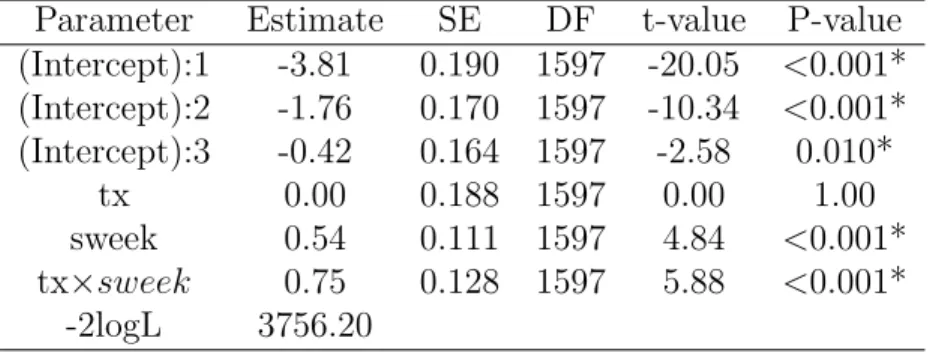
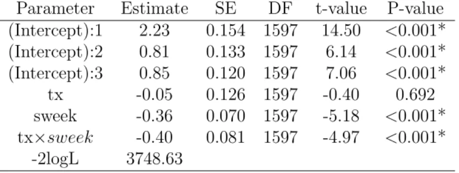
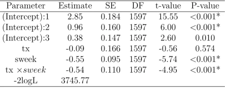
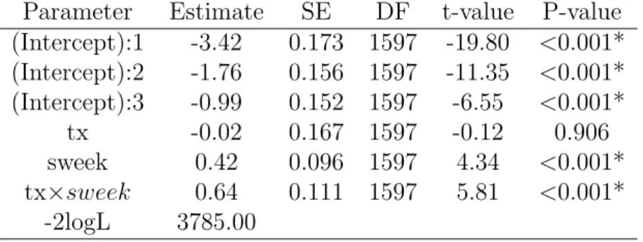
The Schizophrenia data described in [Hedeker and Gibbons, 2006] is from a collaborative study conducted at the National Institute of Mental Health. In this longitudinal study, a total of 1603 observations were obtained from 437 patients. For now, we tentatively ignore the correlations between multiple measurements from the same patient and assume the independence of observations. The outcome was measured as the Inpatient Multidimensional Psychiatric Scale (IMPS)[Lorr and Klett, 1966], which was a eight-category scale ranging from normal (0) to extremely ill (7) that assessed the severity of illness. Hedeker and Gibbons [2006] modified the original scale by aggregating several categories and summarizing it into a four-category measurement ranging from 1 to 4 with 1) normal or borderline mentally ill, 2) mildly or moderately ill, 3) markedly ill, and 4) severely and most extremely ill. Table 1.1 summarizes the distribution of the modified IMPS score. It is of interest to study whether the intervention and time of measurements have a significant impact on the change of IMPS score. To explore this, we fit cumulative logit, adjacent-category, backward continuation ratio and forward continuation ratio ordinal models. To evaluate the concordance of parameter estimates from different computational tools, we wrote our own R code and compared our results to the results from the R package VGAM and to SAS. Tables 1.2, 1.5, 1.8 and 1.11 present the parameter estimates from our code. Tables 1.3, 1.6, 1.9 and 1.12 present the

(40)

parameter estimates from the R package VGAM. Tables 1.4, 1.7, 1.10 and 1.13 present the parameter estimates from SAS. The parameter estimates from the three approaches achieve good concordance, from which we can draw conclusions that the drug and time interaction is significant with an extremely small p-value, which can be interpreted as the distribution of the IMPS score changes more dramatically in intervention group compared to that in the control group. As the interaction is significant, the main effects can not be interpreted according to p-value directly. Instead, we interpret the drug and time main effects based on contrasts. The drug effect βdrug represents the difference of IMPS score distributions

between two groups at baseline (week 0) where the proportion of normal, mildly, markedly and severely ill subjects are similar in two groups. The time effect βtime describes the

significant change of IMPS score distribution as the study continuous. As the drug effect

(41)

Table 1.1: Summary of IMPS score(modified) in the NIMH Schizophrenia data IMPS Score 1 2 3 4 Total

190 474 412 527 1603

Table 1.2: R code for fitting the cumulative logit ordinal model using NIMH Schizophrenia data

Parameter Estimate SE DF t-value P-value (Intercept):1 -3.81 0.189 1597 -20.10 <0.001* (Intercept):2 -1.76 0.170 1597 -10.37 <0.001* (Intercept):3 -0.42 0.163 1597 -2.59 0.010* tx 0.00 0.188 1597 0.00 1.00 sweek 0.54 0.111 1597 4.85 <0.001* tx×sweek 0.75 0.127 1597 5.89 <0.001* -2logL 3756.20

Table 1.3: R package VGAM for fitting the cumulative logit ordinal model using NIMH Schizophrenia data

Table 1.4: SAS output for fitting the cumulative logit ordinal model using NIMH Schizophre-nia data

(42)

Table 1.5: R code for fitting the adjacent categories ordinal model using NIMH Schizophrenia data

Parameter Estimate SE DF t-value P-value (Intercept):1 2.23 0.154 1597 14.50 <0.001* (Intercept):2 0.81 0.133 1597 6.14 <0.001* (Intercept):3 0.85 0.120 1597 7.06 <0.001* tx -0.05 0.126 1597 -0.40 0.692 sweek -0.36 0.070 1597 -5.18 <0.001* tx×sweek -0.40 0.081 1597 -4.97 <0.001* -2logL 3748.63

Table 1.6: R package VGAM for fitting the adjacent categories ordinal model using NIMH Schizophrenia data

Table 1.7: SAS output for fitting the adjacent categories ordinal model using NIMH Schizophrenia data

(43)

Table 1.8: R code for fitting the backward continuation ratio ordinal model using NIMH Schizophrenia data

Parameter Estimate SE DF t-value P-value (Intercept):1 2.85 0.184 1597 15.49 <0.001* (Intercept):2 0.96 0.160 1597 5.97 <0.001* (Intercept):3 0.38 0.147 1597 2.59 0.010 tx -0.09 0.166 1597 -0.56 0.574 sweek -0.55 0.095 1597 -5.73 <0.001* tx ×sweek -0.54 0.110 1597 -4.95 <0.001* -2logL 3745.77

Table 1.9: R package VGAM for fitting the backward continuation ratio ordinal model using NIMH Schizophrenia data

Table 1.10: SAS output for fitting the backward continuation ratio ordinal model using NIMH Schizophrenia data

(44)

Table 1.11: R code for fitting the forward continuation ratio ordinal model using NIMH Schizophrenia data

Parameter Estimate SE DF t-value P-value (Intercept):1 -3.42 0.173 1597 -19.80 <0.001* (Intercept):2 -1.76 0.156 1597 -11.35 <0.001* (Intercept):3 -0.99 0.152 1597 -6.55 <0.001* tx -0.02 0.168 1597 -0.12 0.906 sweek 0.42 0.096 1597 4.34 <0.001* tx×sweek 0.64 0.111 1597 5.81 <0.001* -2logL 3785.04

Table 1.12: R package VGAM for fitting the forward continuation ratio ordinal model using NIMH Schizophrenia data

Table 1.13: SAS for fitting the forward continuation ratio ordinal model using NIMH Schizophrenia data

(45)

Chapter 2 Regularization Methods for

High-dimensional Data

In this chapter, we introduce statistical learning algorithms that are useful for prediction and feature selection problems for high-dimensional data where the number of covariates p

is much larger than the number of samples n. This type of data is particularly prevalent in computational biology where high-throughput genomic technologies plays an increasingly important role in medical research and clinical practice. The statistical learning algorithms produce penalized estimates of coefficients for ‘important’ covariates while shrinking the rest to be exactly zero. This approach has been demonstrated to have superior performance over the traditional hypothesis-based variable selection methods such as Best subsets, Forward Selection and Backward Elimination,etc. It also has better performance in aspects of predic-tion and classificapredic-tion accuracy, stability and consistency for feature selecpredic-tion in data with complex patterns.

(46)

The rest of Chapter 2 is organized as follows: In Section 2.1, we briefly review several existing regularization methods that are applicable for continuous responses. In Section 2.2, we present regularization methods that are suitable for dichotomous responses. In Section 2.3, we discuss the optimization algorithm to solve the regularization path in LASSO. Some comparisons between the LASSO and Forward Stagewise methods are discussed in Section 2.4.

2.1 Regularization Methods for Continuous Response

In high-dimensional data, the explosion of dimensionality allows much more information to be examined simultaneously. In the meantime, the curse of dimensionality raises chal-lenges rarely occurred in low-dimensional settings, such as: data sparsity, high-volatility, and nonlinearity. Variable selection and assessment is an important first step to reduce dimensionality such that fewer important factors can be implemented in a general statis-tical framework. Some traditional variable selection methodologies including Best subsets, Forward Selection and Backward Elimination etc. often fail to provide feasible and stable results due to strong assumptions on covariate independence as well as problematic discrete procedures which yield high variability. The regularization methods, also known as penal-ized models which trade off unbiasedness for lower variability, have demonstrated superior performance in analyzing high-dimensional data. We first review the regularization model framework in the linear model setting.

(47)

Consider a linear model of the form (2.1.1)

yi =xiTβ+i (2.1.1)

where yi is the response for the ith observation, xiT = (1, xi1,· · · , xip) is a vector of the

intercept and p covariates, β = (β0, β1,· · · , βp) is the vector of coefficients associated with

the intercept and covariates, andi is the error term assumed to follow a normal distribution

with mean 0 and varianceσ2_{. The residual sum of square (RSS) in a linear model is defined as}

(2.1.2). It can be shown that the ordinary least squares (OLS) estimator ofβ is the solution that minimizes the RSS. The ordinary least squares estimator has some appealing statistical properties. First, it is also the maximum likelihood estimator for a linear regression model. Second, it is an unbiased estimator where E( ˆβ) =β.

RSS(β) =

n X

i=1

(yi−xiTβ)2 (2.1.2)

In a high-dimensional setting or when data are highly correlated, retaining the unbiased-ness of the estimator is either infeasible or could result in very high variability. Fan and Li [2001] proposed penalized least squares as shown in (2.1.3)

Q(β) =

n X

i=1

(yi−xiTβ)2 +pλ(β) (2.1.3)

where pλ(·) is the penalty function and λ is a tuning parameter that regulates the amount

of shrinkage. Different penalty functions lead to different penalized models. The well known shrinkage procedure ridge regression [Hoerl and Kennard, 1970], which is also known as

(48)

L2−norm penalized regression model, has a penalty function pλ(β) = λP_jβj2. The ridge

regression produces the penalized estimates for all coefficients by sacrificing a little bit un-biasedness in return for smaller variance. As pointed out by Myers [1990], ridge regression is particularly useful for solving the multicollinearity problem in linear regression. However, ridge regression neither performs variable selection nor builds a parsimonious model since it cannot shrink the coefficient estimates to be exactly zero. Alternatively, Tibshirani [1996] proposed the famous Least Absolute Shrinkage and Selection Operator (LASSO) method which sets the penalty function to be theL1 norm of the coefficients wherepλ(β) =λP_j|βj|.

LASSO has been demonstrated to be useful in variable selection since it can shrink the coeffi-cient estimates associated with unimportant covariates to be exactly zero while producing pe-nalized estimates for the few important covariates. The pepe-nalized estimates also yield better prediction accuracy in terms of smaller prediction error. In addition, Zou and Hastie [2005] introduced the elastic net penalty pλ(β) = λ[(1−α)

P

j|βj|+α P

jβ

2

j] which improves the

stability of the LASSO when exposed to a group of strongly correlated predictors. Moreover, Fan and Li [2001] advocated a penalty function from a different mechanism called smoothly clipped absolute deviation (SCAD) with a form p0_λ(β) = λ I(β ≤ λ) + (αλ−β)+

(α−1)λ I(β > λ)

where α and λ are the unknown parameters determined by cross-validation. This method is shown to be effective without creating excessive biases especially in situations where the noise to signal ratio is low.

In this Section we concentrate on theL1penalized regression model LASSO and two other

popular algorithms: Least Angle Regression [Efron et al., 2004] (better known as ‘LAR’) and incremental forward stagewise regression [Hastie et al., 2007] which were also proposed for

(49)

solving the penalized least squares problem when the response is continuous.

2.1.1 LASSO

The LASSO, also known as theL1 penalized regression model proposed by Tibshirani [1996],

is a widely used smooth optimization technique for building a parsimonious model from high-dimensional data. It produces penalized estimates for the unknown parameters β as shown in (2.1.4) ˆ βLASSO = argmin{ n X i=1 (yi−β0−xiTβ)2+λ p X j=1 |βj|} (2.1.4)

where the tuning parameter λ controls the amount of shrinkage. The penalized estimates are equivalent to the ordinary least squares estimates if λ = 0 and the penalized estimates are all 0 if λ → ∞. Therefore, the choice of the turning parameter λ can be thought of as a way to determine the number of important predictors. As there is no standard criteria associated with the choice of λ, λ can be the one associated with optimum model fitting criteria (AIC, BIC) or that leads to the smallest cross-validation error decrease.

The rationale behind the LASSO can be illustrated by Figure 2.1 reproduced from [Tib-shirani, 1996] which also helps explain the mechanism of variable selection. Figure 2.1 illustrates a situation when there are two covariates x1,x2 in the linear regression model.

The blue diamond area is defined by the penalty function|β1|+|β2| ≤t, wheretis a scale

(50)

the penalized estimate and the ordinary least squares estimate. To illustrate, we assume the data is normalized so that x1Tx2 = 0. We define the squared error as follows (2.1.5)

n X i=1 (xiβˆP LS −xiβÔLS)2 = n X i=1 ( ˆβP LS₋_β_ÔLS₎T_x iTxi( ˆβP LS −βÔLS) = ( ˆβ₁P LS −βˆ₁OLS,βˆ₂P LS −βˆ₂OLS)    x1Tx1 0 0 x2Tx2       ˆ βP LS 1 −βˆ1OLS ˆ βP LS 2 −βˆ2OLS    = ( ˆβ₁P LS −βˆ₁OLS)2x1Tx1+ ( ˆβ2P LS −βˆ2OLS)2x2Tx2 =k (2.1.5)

where x1Tx1 = Pn_i₌₁x2i1,x2Tx2 = Pn_i₌₁x2i2 and k is a constant. The last line of equation

(2.1.5) defines several ellipses that are centered at ˆβ = ( ˆβOLS

1 ,βˆ2OLS). As the penalized

estimates have to satisfy both equation (2.1.5) and the penalty function, a possible situation is when the contour hits the corner of the diamond which yields an exact zero estimate for one coefficient. From here, it is not difficult to generalize to a higher dimensional scenario when multiple coefficients are shrunk to be exactly zero.

(51)

2.1.2 Forward Stagewise Method

The forward stagewise method is a greedy procedure similar to forward stepwise but more cautious. It was historically known as an ‘inefficient’ procedure since the model is updated by a very small incremental step at each iteration. Recently, it is gained enormous atten-tion when Hastie et al. [2007] linked forward stagewise to a version of boosting proposed by Schapire et al. [1998] for linear models. This ‘slow fitting’ turns out to be quite com-petitive in terms of variable selection stability and prediction accuracy. In fact, Efron et al. [2004] showed the forward stagewise profile can be similar or even identical to the LASSO path under certain conditions and thus can be used to solve the penalized regression problem.

The forward stagewise method for linear regression is as follows:

1. Standardize the covariates so that each has mean 0 and unit norm. At the initial step, set the residual vector r toy and β = (β1,· · · , βp) =0.

2. Calculate the correlation between xj forj = 1,· · · , pand the current residualr. Select

the xj most correlated withr.

3. Update the corresponding coefficient βj with βj ←βj+·sign <xj,r> where is a

small amount, e.g. = 10−4 and <xj,r > represents the correlation between xj and

r.

Update the residual tor ←r−·sign <xj,r>xj.

4. Repeat steps 2 and 3 many times untilris uncorrelated or at least not highly correlated with any of the covariates.

(52)

The mechanism of forward stagewise can be explained by Figure 2.2 reproduced from Hastie et al. [2009]. Recall in the linear regression model, the OLS estimator ˆβ is the estimate associated with minimal residual sum-of-squares (RSS)(2.1.2). In projection presentation, suppose responseyis projected onto the space spanned by covariatesx1andx2. The residual

r = y−yˆ measures the distance between y and the predictor space. The RSS is achieved when the residual r is orthogonal to both x1 and x2, in other words, r is uncorrelated with

all the covariates in model. The mechanism can be easily generalized to a high-dimensional scenario. In the forward stagewise procedure discussed above, the update of coefficients

β and residual r stops when r is uncorrelated, or at least not highly correlated with any of the covariates in the model, and can be interpreted as when the minimum RSS is reached.

Figure 2.2: Least square projection in linear regression model

2.1.3 LAR

LAR, which stand for ‘Least Angle Regression’ proposed by Efron et al. [2004], is considered as a more ‘democratic’ version of the forward stagewise method. After selecting the predic-tor that is most correlated with the residual, rather than taking the full step towards that direction, LAR takes the largest step possible in that direction until some other predictor has

(53)

reached the correlation with the current residual. Then the two predictors are moved in the joint least squares direction until the third predictor achieves the amount of correlation with the current residual and joins the selected group. This procedure is repeated many times until the correlation of each predictor to the current residual is smaller than a threshold. This new comer is known to be closely connected to LASSO and provides a more efficient solution to the penalized least squares problem.

2.2 Regularization Methods for Dichotomous Responses

In this section, we move on to discuss regularization methods implemented for the logistic regression model with high-dimensional predictors by first providing the statistical framework for logistic regression in the traditional setting. Consider a logistic regression of the form (2.2.1) log P(Yi = 1|x) P(Yi = 0|xi) = log π(xi) 1−π(xi) =α+xiTβ (2.2.1)

where yi = 1 indicates 1 success and yi = 0 indicates failure. For each observation i,

we denote Yi being the total number of successes and 1 −Yi being the total number of

failures. Therefore, Yi follows a binomial distribution with mass function f(Yi; 1, πi) =

1

Yi

πYi

i (1−πi)1−Yi. xiT = (xi1,· · · , xip) is a vector ofpcovariates,αrepresents the intercept,

andβ= (β1,· · · , βp) is a vector of coefficients associated with the covariates. The maximum

(54)

the model. The likelihood function for the logistic regression model can be written as: L(α,β|xi) = N Y i=1 π(xi)Yi(1−π(xi))1−Yi = N Y i=1 exp(α+xiTβ) 1 + exp(α+xiTβ) Yi 1 1 + exp(α+xiTβ) 1−Yi . (2.2.2)

Correspondingly, the log-likelihood can be written as:

logL(α,β|xi) =

N X

i=1

Yilogπ(xi) + (1−Yi) log(1−π(xi)). (2.2.3)

It is not hard to show that logL(α,β|xi) in (2.2.3) is a concave function and its negative, −logL(α,β|xi) is a convex function.

2.2.1 LASSO for Logistic Regression

In a high-dimensional setting where N p, maximum likelihood estimation is no longer feasible due to singularities in the Hessian matrix. The penalized model is again proposed and demonstrated to be useful in this case. Recall for the linear regression model with high-dimensional covariates the penalized estimator is the one associated with the optimum value of the penalized least squares (2.1.3), which consists of the residual sum of squares and the penalty function. Notice the residual sum of squares is the kernel of the likelihood in the linear model case. When the response is discrete, minimizing the residual sum of square is not reasonable, so a modified penalized model that maximizes the penalized log-likelihood function was proposed [Wu et al., 2009]. The penalized log-log-likelihood consists of