September 2009, Volume 31, Issue 10. http://www.jstatsoft.org/
CircStat
: A
MATLAB
Toolbox for Circular Statistics
Philipp Berens
Max Planck Institute for Biological Cybernetics
Abstract
Directional data is ubiquitious in science. Due to its circular nature such data cannot be analyzed with commonly used statistical techniques. Despite the rapid development of specialized methods for directional statistics over the last fifty years, there is only little software available that makes such methods easy to use for practioners. Most impor-tantly, one of the most commonly used programming languages in biosciences,MATLAB, is currently not supporting directional statistics. To remedy this situation, we have im-plemented the CircStattoolbox forMATLABwhich provides methods for the descriptive and inferential statistical analysis of directional data. We cover the statistical background of the available methods and describe how to apply them to data. Finally, we analyze a dataset from neurophysiology to demonstrate the capabilities of theCircStattoolbox.
Keywords: circular statistics, directional statistics, rayleigh test, MATLAB.
1. Introduction
Circular statistics is a subfield of statistics, which is devoted to the development of statistical techniques for the use with data on an angular scale. On this scale, there is no designated zero and, in contrast to a linear scale, the designation of high and low values is arbitrary. Consider for example the case of wind directions measured in degrees — wind blowing towards 359 deg follows almost the same path as wind blowing towards 0 deg. In addition to measurements which are naturally measured in angles circular statistics applies also to types of data such as time of the day, phase of the moon or day of the year that exhibit a different periodicity. Such data is encountered in many fields of science as diverse as physics (van Doorn, Dhruva, Sreenivasan, and Cassella 2000), geoscience (Bowers, Morton, and Mould 2000), agricultural sciences (Aradottir, Robertson, and Moore 1997), neuroscience (Maldonado, Godecke, Gray, and Bonhoeffer 1997;Froehler and Duffy 2002), zoology (Boles and Lohmann 2003;Cochran, Mouritsen, and Wikelski 2004), medical research (Le, Liu, Lindgren, Daly, and Giebink 2003; Gao, Chia, Krantz, Nordin, and Machin 2006), computer science (Hanbury 2003), psychology
(Kubiak and Jonas 2007), criminology (Brunsdon and Corcoran 2005) or political and social sciences (Haskey 1988;Gill and Hangartner 2008). For example,Cochranet al.(2004) investi-gate whether the sense of orientation of night-migrating birds could be disrupted by exposing them to strong magnetic pulses. While the animals naturally fly in northerly directions, birds exposed to eastwards oriented magnetic fields flew westwards.
The circular nature of such data prevents the use of commonly used statistical techniques, as these would provide wrong or misleading results. The authors thus used tools from circular statistics to compute the average heading direction, assert the prevalence of a common heading direction for a group of birds and compare the average heading directions of an experimentally manipulated and a control group. The development of techniques suitable to this end started in the early 1950es with a seminal paper by Fisher (1953). Despite the fact that circular statistics is still in very active development, several monographs and textbook lay out a standard repertoire of circular statistics methods (e.g., Batschelet 1981; Fisher 1995; Zar 1999;Jammalamadaka and Sengupta 2001).
It is all the more surprising that techniques for the analysis of circular data have not yet become available as part of many commerical software products for data analysis such as MATLAB.MATLABis a high-level programming environment designed for numerical compu-tations developed and marketed by The Mathworks (The MathWorks, Inc. 2007). It is highly popular among many scientists in biomedical research and beyond, since it offers a wide range of preimplemented functionality. Currently it is used by more than one million people (Moler 2006). More specialized add-on packages are available in the form of toolboxes. The statis-tics toolbox (The MathWorks, Inc. 2008), for example, extends the capabilities of the core system by providing functions for many commonly encountered problems in descriptive and inferential statistics. Methods for the analysis of circular data, however, are not part of this, or any other, toolbox for MATLAB. TheCircStat toolbox described in this paper is intended to provide the users of MATLABwith a comprehensive set of functions and solutions for most common problems in descriptive and inferential statistics for circular data1.
While the software package described in this paper is currently the only one offering circular statistics for the use with MATLAB, there are a small number of comparable toolboxes for other languages or environments. TheCircStatspackage for the Rprogramming language is most closely related to the toolbox described here (Lund and Agostinelli 2007). It offers a small number of tests as described in (Jammalamadaka and Sengupta 2001) and has been ported from a S-plus original version. While R is hugely popular among statisticians, MATLAB is the most commonly used programming and data analysis environment in the engineering and biological sciences. A similar package is available forStata(Cox 2004). Both of these packages are open source and freely available on the internet. In addition, Oriana is a commerically available program which offers basic functionality for the analysis of circular data (Kovach Computing Services 2009).
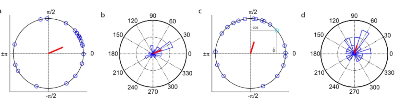
In the following, we will describe the methods implemented in the CircStat toolbox and explain how they can be used for analysis of circular data. The exposition will be fairly detailed as we combine a set of methods described in various different sources. First, we start with descriptive statistics, before we cover important methods from inferential statistics and measures of association. For illustrations and examples, we will mostly be referring to two synthetic datasets shown in Figure1. Both datasets are shown in raw format as well as in the
0 π/2 ±π -π/2 a 0 π/2 ±π -π/2 c 30 210 60 240 90 270 120 300 150 330 0 0 8 1 b 30 210 60 240 90 270 120 300 150 330 0 0 8 1 d cos sin
Figure 1: Example datasetsα (a,b) andβ (c,d) used throughout the paper. Both datasets consist of N = 20 samples. In a and c, data is shown as points on the unit circle. In b and d, angular histograms are shown. Red lines indicate the direction and magnitude of the mean resultant vector. Grey lines in c serve to illustrate the cosine and sine component of an angular datapoint.
form of histograms. The dataset shown in Figure 1a and b will be calledα and the dataset shown in Figure1c and d will be calledβ. Finally, we will apply the methods described in this paper to a dataset from a neuroscientific context and use them to study orientation tuning of single neurons. First, however, we discuss some notational conventions and cover some basic issues.
We denote a vector of N directional observations αi as α = (α1, . . . , αN). All functions
described in this paper take their arguments in radians. To convert angles in degrees to angles in radians we compute
αdegree = 360 deg·αradians
2π . (1)
Conversions from degrees to radians and vice versa can be performed using the functions circ_ang2rad(alpha) and circ_rad2ang(alpha).
Similarly, data such as time of the day or phase of the moon can be converted to a common angular scale in radians by
α= 2πx k ,
where x is the representation of the data in the original scale, α is its angular direction and k is the total number of steps on the scale that y is measured in. For example, we have x representing day of the year and thus k = 365, not considering leapyears for simplicity. In addition, data with multiple modes—known as axial data—can be converted to a unimodal sample for the purpose of certain analysis such as computation of a mean resultant vector by (Fisher 1995, Section 2.4.). For p-axial data this results in the following mapping:
αi −→pαi(mod2π)
Afterwards, the result of the performed computation can be transformed back to the original scale. This operation is implemented in circ_axial.
2. Descriptive statistics
In this section we describe the methods and functions implemented in theCircStattoolbox for computing descriptive measures on angular data. They can be used to explore and summarize important properties of a sample of angular data such as central tendency, spread, symmetry or peakedness.
If not otherwise noted, all functions can also be applied to binned data if supplied with a second optional input argumentw of the same length as α. They then assume that the data has been binned with bin center i equal to αi and wi equal to the number or fraction of
samples falling into bin i. For measures of dispersion, the bin width can be specified as an optional third argument, which is then used for bias correction.
Mean The mean of a sampleα cannot be computed by simply averaging the data points. Consider for example calculating the mean of a set of three angles, 10 deg,30 deg and 350 deg. The arithmetic mean of the angles is clearly 130 deg, while all data samples point towards 0 deg.
Instead, directions are first transformed to unit vectors in the two-dimensional plane by ri = cosαi sinαi .
This is illustrated in Figure 1a and c, where all datapoints marked by circles lie on the unit sphere. As indicated for the light blue point in Figure1c, the x-coordinate of a point corresponds to the cosine of the angle and the y-coordinate to the sine.
After this transformation, the vectorsri are vector averaged by
¯ r = 1 N X i ri.
The vector ¯r is called mean resultant vector. To yield the mean angular direction ¯α, ¯r is transformed using the four quadrant inverse tangent function. For further illustraction, see also the example in Figure2.
InCircStat, the mean resultant vector ¯α of a set of datapoints can be computed by >> alpha_bar = circ_mean(alpha);
For the example, this results in mean resultant vectors pointing towards ¯α = 23.5 deg and ¯
β= 72.5 deg, respectively. These vectors are also shown in red.
For ease of implementation in MATLAB, the first transformation is implemented exploiting the identity
cosα+isinα= exp(iα)
and the second transformation uses theMATLABfunctionangle. If a second and third output argument are requested,circ_meancomputes the 95% confidence intervals on the estimation of ¯α using circ_meanconf.
a
b
c
Figure 2: Illustration of the resultant vector and the resultant vector length. In a, three samples 60,180,300 deg (black) yield a resultant vector length of zero, since the points are exactely uniformly spaced around the circle. In b, 120,180,240 deg result in a resultant vector length of 2/3, with a common mean direction of π. In c, 150,180,210 deg yield a resultant vector length of 0.9107 with the same mean direction. Resultant vectors are shown in grey and can be obtained by vector addition. The light grey circle is the unit circle.
Median The median direction ˆα of a sample α is the direction for which half of the data-points fall on either side. For circular data thus the diameter of the circle that divides the data into two equal sized groups is found. The median is the endpoint of the diameter closer to the center of mass of the data. If N is even, it lies half-way between the two closest datapoints. If N is odd, it falls on one of the data points.
If the datapoints are drawn from a uniform distribution or evenly spaced around the circle there is no well-defined median direction.
In CircStat, the median of a dataset is computed by >> alpha_hat = circ_median(alpha);
For the example, we obtain ˆα = 27 deg and ˆβ = 76 deg. The median cannot be computed for binned data.
Resultant vector length The length of the mean resultant vector is a crucial quantity for the measurement of circular spread or hypothesis testing in directional statistics. The closer it is to one, the more concentrated the data sample is around the mean direction. For an example, see Figure 2. The resultant vector length is computed by
R=kr¯k. In CircStat, the resultant vector length is computed by >> R = circ_r(alpha);
The estimation of R is biased when binned data is used. This bias can be corrected for by supplying the bin spacing das a third optional argument and computing a correction factor (Zar 1999, Equation 26.16)
c= d
2 sin(d/2), settingRc=cR.
Variance The circular variance is closely related to the length of the mean resultant vector. It is defined as
S = 1−R.
In contrast to the variance on a linear scale, the circular variancesis bounded in the interval [0,1]. It is indicative of the spread in a data set. If all samples point into the same direction, the resultant vector will have length close to 1 and the circular variance will correspondingly be small. If the samples are spread out evenly around the circle, the resultant vector will have length close to 0 and the circular variance will be close to maximal. Importantly, however, a circular variance of 1 does not imply a uniform distribution around the circle. If all samples either point towards 0 deg or 180 deg, the resultant vector length is 0, yet the data is not distributed uniformly around the circle.
In CircStat, the circular variance is computed using >> S = circ_var(alpha);
In the example, we thus obtainSα = 0.55 undSβ = 0.64. Thus the datasetβ is more spread
out than dataset β.
Standard deviation Interestingly, multiple quantities have been introduced as analogues to the linear standard deviation. First, the angular deviation is defined as
s=p2(1−R).
This quantity lies in the interval [0,√2]. Alternatively, the circular standard deviation is defined as
s0=√−2 lnR
and ranges from 0 to ∞. Generally, the first measure is preferred, as it is bounded, but the two measures deviate littleZar(1999).
InCircStat, the angular deviation is computed as >> s = circ_std(alpha);
and the circular standard deviation as
>> s0 = circ_std(alpha,[],[],'mardia');
Trigonometric moments It is possible to compute the p-th trigonometric moment of a sample of circular data (Fisher 1995). The uncentred p-th moment is given by
m0p= 1 N N X i=1 cospαi+i 1 N N X i=1 sinpαi.
Similarly, the centred trigonometric moments are obtained by calculating the moments relative to the sample mean by
mp = 1 N N X i=1 cosp(αi−α¯) +i 1 N N X i=1 sinp(αi−α¯).
Similar to the mean resultant vector,m0p and mp can be decomposed into direction ¯αp and
magnitudeRp.
InCircStat, the uncentredp-th trigonometric moment can be found by calling >> mp = circ_moment(alpha,[],p);
and the centred p-th trigonometric moment by >> mp = circ_moment(alpha,[],p,true);
Optionally, direction and magnitude are returned as second and third output argument.
Skewness As a measure of symmetry, circular skewness can be computed as (Pewsey 2004)
b= 1 N N X i=1 sin 2(αi−α¯).
A value close to 0 is indicative of a symmetric population around the mean direction. Alter-natively, a standardized measure of skewness has been defined as (Fisher 1995)
b0= R2sin( ¯α2−2 ¯α) (1−R)2/3 InCircStat, circular skewness is computed by
>> [b, b0] = circ_skew(alpha);
For the example, we find that both samples are relatively symmetric around their mean directions with skewness values ofbα= 0.02 andbβ = 0.04 orb0,α=−0.019 andb0,β=−0.099.
Kurtosis As a measure of peakedness, circular kurtosis can be computed as (Pewsey 2004)
k= 1 N N X i=1 cos 2(αi−α¯).
A large positive sample value of k close to one indicates a strongly peaked distribution. Alternatively, a standardized measure of kurtosis has been defined as (Fisher 1995)
k0= R2cos( ¯α
0
2−2 ¯α)−R4 (1−R)2 .
The former definition is intuitively appealing, since many values close to the mean direction lead to positive contributions to the above average due to the shape of the cosine function. However, the latter definition has the appealing property that data generated by a von Mises distribution, which is the circular analogue of the Normal distribution, hask0 = 0.
InCircStat, circular kurtosis is computed by >> [k k0] = circ_kurtosis(alpha);
For the example, we find thatkα = 0.42 and kβ = 0.01, such that sample β is less peaked
than sample α. If we want to compare the peakedness of the two samples to a von Mises distribution, we find that both samples have lower kurtosis with k0,α = −0.66 and k0,β =
−1.18.
3. Inferential statistics
In this section, we describe a set of functions implemented inCircStatfor inferential statistics with angular data. The first set of functions allows to test the popular question of circular uniformity, while other methods allow to investigate more specific hypothesis about the mean direction of one or multiple samples. For example, researchers studying the migratory be-havior of birds (Wiltschko and Wiltschko 1972;Cochranet al.2004) might want to establish that all animals from one species indeed migrate into a common direction or acertain that two species of birds migrate into differing directions.
3.1. Testing for circular uniformity
A common question in circular statistics is whether a data sample is distributed uniformly around the circle or has a common mean direction. There are multiple tests for this problem that share a common null hypothesis
H0: The population is distributed uniformly around the circle with alternative hypothesis
HA: The population is not distributed uniformly around the circle.
They differ in their efficiency to detect certain departures from uniformity, as discussed below.
Rayleigh test The Rayleigh test asks how large the resultant vector lengthR must be to indicate a non-uniform distribution (Fisher 1995). It is particularly suited for detecting a unimodal deviation from uniformity. If the data indeed is unimodal, it is the most powerful test described in this section.
The approximate p-value underH0 is computed as (Zar 1999, Equation 27.4) P = exphp(1 + 4N + 4(N2−R2
n)−(1 + 2N) i
,
where Rn = R·N. This approximation is valid up to three decimal places for N as small
as 10. The Rayleigh test can also be applied to axial data after suitable transformation. Importantly, it assumes sampling from a von Mises distribution.
InCircStat, the Rayleigh test is performed by computing >> p = circ_rtest(alpha);
where a smallp indicates a significant departure from uniformity and indicates to reject the null hypothesis.
For the examples, we find that at the 0.05 significance level, the null hypothesis can be rejected for sampleα (P = 0.02), while for sampleβ, this is not the case (P = 0.08).
Omnibus test The “omnibus test” or Hodges-Ajne test (Zar 1999) for circular uniformity is an alternative to the Rayleigh test that works well for unimodal, biomodal and multi-modal distributions. It is able to detect general deviations from uniformity at the price of some statistical power. Also, it does not make specific assumptions about the underlying distribution.
To conduct the test, the smallest numbermthat occur within a range of 180 deg is computed. Under the null hypothesis, the probability of observing anm this small or smaller is
P = 1 2N−1(N−2m) N m , which can forN >50 be approximated by
P ' √ 2π A exp −π 2/(8A2) , whereA= π √ N 2(N−2m).
In CircStat, the Omnibus test is performed by computing >> p = circ_otest(alpha);
For the examples, we find that at the 0.05 significance level, the null hypothesis cannot be rejected for either sample (P = 0.11 and P = 0.3, respectively).
Rao’s spacing test Rao’s spacing test for circular uniformity is an additional alternative to the Rayleigh test (Batschelet 1981). It is more powerful than alternatives when the data are neither unimodal nor axially bimodal. It is based on the idea that in an ordered sample α = (α1, . . . , αN) withαi+1> αi sampled from a uniform distribution the differences between
successive samples should be approximately 360N◦. Its test statistic is defined as
U = 1 2 N X i=1 |di−λ|,
with di = αi+1 −αi, dN = 360◦ −(αN −α1) and λ = 360
◦
N . The distribution of U is
computationally very complex, and we use tabled values instead of the full distribution as computed by (Russell and Levitin 1995).
In CircStat, Rao’s spacing test is performed by >> p = circ_raotest(alpha);
For the examples, we find that, at the 0.05 significance level, the null hypothesis cannot be rejected for either sample (P ≥0.05).
V test The V test for circular uniformity is similar to the Rayleigh test with the difference that under the alternative hypothesis HAis assumed to have a known mean direction ¯αA. It
is important that the mean direction has to been known in advance, i.e., before any look at the data is taken. The test statistic is computed as (Zar 1999)
V =Rncos( ¯α−α¯A),
whereRn as above. Approximate critical values for the quanitity
V
r
2 N
can be obtained from the one tailed normal deviate Zα(1). Due to the additional information used, the V test is more powerful than the Rayleigh test. The additional power comes at a certain cost: Not rejecting the null hypothesis in this case leaves it open whether the cause for that failure was insufficient evidence for non-uniformity or a different mean direction than ¯
αA.
InCircStat, the V test is performed by >> p = circ_vtest(alpha,0);
Testing for violations of uniformity assuming a mean direction of 0 deg results in a rejection of the null hypothesis for α (P = 0.045), but not β (P = 0.25). In the latter case we thus do not know whether the reason for not rejecting the null hypothesis was that the preferred direction was misspecified or because the sample is indeed uniformly distributed around the circle.
3.2. Tests concerning mean and median
This section covers a more diverse set of tests concerning various hypotheses about the mean or median direction. For example, they can be used to place confidence intervals on the mean direction, test for specific mean or median direction or for symmetry around the median.
Confidence Intervals for the Mean Direction We compute the (1−δ)%-confidence intervals for the population mean (Zar 1999, Equations 26.23-26.26). For R ≤0.9 andR >
q χ2δ,1/2N, we compute d= arccos r 2N(2R2 n−N χ2δ,1) 4N−χ2 δ,1 Rn ,
whereRn=R·N. ForR >0.9, we compute
d= arccos q N −(N2−R2 n) exp(χ2δ,1/N) Rn .
In both cases, the lower confidence limit of the mean is found by L1 = ¯α−dand the upper confidence limit by L2 = ¯α+d.
In CircStat, 95%-confidence intervals are found either by calling >> [alpha_bar ul ll] = circ_mean(alpha);
or by computing
>> d = circ_confmean(alpha, 0.05);
and computing the confidence limits as described above.
For the example, we can assert that the true population mean likely lies in the interval 341.5−65.43 deg and 12.73−132.27 deg, respectively for datasets α and β.
One sample test for the mean angle Similar to a one sample t-test on a linear scale, we can test whether the population mean angle is equal to a specified direction.
H0: The population mean angle ¯α is equal to ¯α0.
HA: The population mean angle ¯α is not equal to ¯α0, i.e., ¯α6= ¯α0.
The test at significance levelδ is performed by checking whether ¯α0 ∈ [L1, L2], where L1is the lower 1−δ confidence limit on the population mean and L2 the upper confidence limit (Zar 1999).
InCircStat, this test is performed by
>> p = circ_mtest(alpha,ang2rad(90));
For the example dataset α, we thus can reject the null hypothesis that the true population mean is equal to 90 deg, while we do not have sufficient evidence to reject the hypothesis that it is equal to 0 deg.
Significance of the median angle A nonparametric test with
H0: The population median angle ˆα is equal to ˆα0.
HA: The population median angle ˆα is not equal to ˆα0, i.e., ˆα6= ˆα0.
is performed by applying the binomial test (Zar 1999). To this end, the numbernof samples falling on either side of a diameter through ˆα0 are counted. The p-value for observing this sample under H0 is found by computing the probability of observing n or more out of N samples falling on one side of the diameter under a binomial distributionB(N, p) withp= 0.5. In CircStat, this test is performed by
>> p = circ_medtest(alpha,ang2rad(90));
For the example dataset α, we thus can reject the null hypothesis that the true population mean is equal to 105 deg, while we do not have sufficient evidence to reject the hypothesis that it is equal to 25 deg.
Symmetry around median angle A simple test of symmetry of a sample around the median can be performed by computing the circular distancedi of each point from the median
and subjecting the di to a Wilcoxon signed-rank test (Zar 1999). It has the hypothesis set
H0: The underlying distribution is symmetrical around ˆα. HA: The underlying distribution is not symmetrical around ˆα.
The Wilcoxon signed-rank test asks whether the median of the circular distances di is zero.
In CircStat, testing for symmetry around the median angle is performed by >> p = circ_symtest(alpha);
For the two datasets in the example, the null hypothesis cannot be rejected (P = 0.84 and P = 0.79), in line with the measurements of skewness close to zero above.
3.3. Paired and multisample tests
In this section, we will describe three methods for two- or multisample analysis concerning the mean or median direction with one or two factors. In the one-factor case, a parametric as well as a non-parametric test are available, while the two-factor case is covered only by a parametric test. We will use a new example , where we draw 30 samples each from three von Mises distributions with concentration parameter κ= 10 and preferred direction ¯θ1=π,
¯
θ2 =π+ 0.25 and ¯θ3 =π+ 0.5.
One-factor ANOVA or Watson-Williams test The Watson-Williams two- or multi-sample test of the null hypothesis is a circular analogue of the two multi-sample t-test or the one-factor ANOVA. Thus, it assesses the question whether the mean directions of two or more groups are identical or not.
H0: All ofsgroups share a common mean direction, i.e., ¯α1=· · ·= ¯αs.
HA: Not all sgroups have a common mean direction.
The test statistic is calculated via (Watson and Williams 1956;Stephens 1969)
F =K (N −s)Ps j=1Rj−R (s−1)N −Ps j=1Rj ,
where R is the mean resultant vector length when all samples are pooled and Rj the mean
resultant vector length computed on thejth group alone (similar to total variance and within group variance in the ANOVA setting). The correction factor K is computed from
K= 1 + 3 8κ,
whereκ is the maximum likelihood estimate of the concentration parameter of a von Mises distribution with resultant vector lengthrw. We compute κ via the approximation given by
Fisher (1995, Section 4.5.5). Here, rw is the mean resultant vector length of thes resultant
vectors rj computed for each group individually. The obtained value of the test statistic is
then compared to a critical value at theδ level obtained fromFδ(1),1,N−2.
The Watson-Williams test assumes underlying von Mises distributions with equal concentra-tion parameter, but has proven to be fairly robust against deviaconcentra-tions from these assumpconcentra-tions (Zar 1999). The sample size for applying the test should be at least 5 for each individual sample. If binned data is used, bin widths should be no larger than 10 deg. Note that re-jecting the null hypothesis only provides evidence that not all of thes groups come from a population with equal mean direction, not if all groups have pairwise differing mean directions or evidence of which of the groups differ.
InCircStat, the Watson-Williams test can be performed in two ways. For two samples, >> p = circ_wwtest(alpha, beta);
compares the two samples directly, while >> p = circ_wwtest(alpha, idx);
uses idx to assign individual samples αi to the groups. If a second output argument is
requested, no ANOVA table is printed but rather returned as a cell structure.
We first apply the test to our example datasets θ1 and θ2, which we find to show a highly significant difference in their mean preferred directions (P <0.001). Next we test for difference between any of the group means ofθ1,θ2 andθ3, which we find also to be highly significantly different (P <10−10).
Multi-sample test for equal median directions We can test a similar nonparametric hypothesis, namely for equal medians amongs groups of samples, using a test suggested by Fisher(1995). It is a circular analogue to the Kruskal-Wallis test.
H0: Any of ssamples share a common median direction, i.e., ˆα1=· · ·= ˆαs.
HA: Not all ssamples have a common median direction.
We first compute the total median direction ˆα by pooling all groups. Then we compute the number mi of samples within the ith group, whose angular distance d(αji,αˆ) to the total
median is negative, where αij indicates the jth sample from theith group. The test statistic is computed as P = N 2 M(N−M) s X i=1 m2i ni − N M N −M.
Here, ni are the number of samples in each group. The obtained statistic is compared to the
upper 1−δ-percentile of a χ2s−1- distribution.
Similar caveats regarding the interpretation of the results hold as for the Watson-Williams test. The test should not be used if any ni <10.
In CircStat, this test can be performed in two ways. For two samples, >> p = circ_cmtest(alpha, beta);
compares the two samples directly, while >> p = circ_cmtest(alpha, idx);
uses idxto assign individual samplesαi to the groups.
For the example, we find that the two groups θ1 andθ2 have a significantly different median orientations (P = 0.005).
Two-factor ANOVA or Harrison-Kanji test In a similar fashion to the one-factor ANOVA, we can also test for the influence of two factors simultaneously. Such a two-factor ANOVA method for circular data has been introduced by (Harrison, Kanji, and Gadsden 1986; Harrison and Kanji 1988). In addition to potential effects of the two factors, we can also study the impact of their interactions on the population means.
The test developed byHarrison and Kanji(1988) treats two situations separately: First, when the pooled sample concentration parameter κ is larger than two. Second, when it is smaller than two. Since the respective test statistics and their derivation is somewhat lengthy, we refer to Harrison and Kanji (1988) for details.
In CircStat, the two-factor ANOVA can be performed in the following way: >> [p, table] = circ_hktest(alpha,idp,idq,true);
Here,alphacontains the whole sample, whileidpandidqindicate the respective level of the two factors. The last argument ensures that the effect of interactions is tested for as well. To illustrate the test, we useθ1 andθ2. Factor A indicates whether a sample belongs toθ1or θ2. Factor B is assigned randomly to the samples of θ1 and θ2. We test for effects of factors A and B as well as their interactions. Since the jointκ≈7.5, the large κmethod is used. As expected from the setup, we find a significant effect of factor A (P <0.001), but no effect of factor B and no interaction effect.
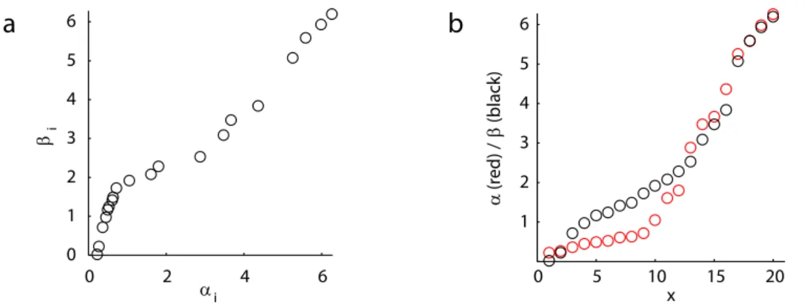
0 2 4 6 0 1 2 3 4 5 6 αi βi 0 5 10 15 20 1 2 3 4 5 6 x α (red) / β (black)
a
b
Figure 3: (a) Datasets α and β plotted against each other as if they had been obtained as paired samples. (b)α (red) and β (black) plotted against their indices 1, . . . ,20. β shows a slightly higher linear association with its index, since it is less peaked.
4. Measures of association
In this section, we describe two functions implemented inCircStatthat can be used to study questions of association where angular data is involved. The first kind of situation is where the correlation between two circular variables is to be assessed, as for example in Berens, Keliris, Ecker, Logothetis, and Tolias(2008), where we used to two different signal—multi-unit spiking activity and local field potentials—and computed the preferred orientation of a visual stimulus for both of them. We used circular-circular correlation to study the relationship between the two signals. The second situation is where the association between a linear and a circular variable is of interest. InBerenset al.(2008), we might have been interested in the relationship between preferred orientation of a site and position of the stimulus on the screen. For illustrations in this section, we resort again to the example shown in Figure 1.
Circular-circular correlation Correlation between two directional variables can be as-sessed by computing a correlation coefficientρcc(Jammalamadaka and Sengupta 2001, p. 176)
by ρcc = P isin(αi−α¯) sin(βi−β¯) q P isin2(αi−α¯) sin2(βi−β¯) ,
whereα and βdenote two samples of angular data and ¯α the angular mean. Significance of this correlation can be assessed by computing a p-value forρcc. Under the null hypothesis of
no correlation, the test statistic
t=pf ·ρcc,
follows a standard normal distribution. The termf is given by f =N P isin2(αi−α¯)Pisin(βi−β¯) P isin2(αi−α¯) sin2(βi−β¯) .
>> [c,p] = circ_corrcc(alpha, beta);
For the example datasetsαandβ, this results in a highly significant correlation ofρcc = 0.67
with P = 0.007 as both samples are ordered (see Figure 3a).
Circular-linear correlation The linear association between a directional random variable α and a linear variable x can be assessed by correlating x with cosα and sinα individually . To this end, we define the correlation coefficients rsx = c(sinα, x),rcx = c(cosα, x) and
rcs = c(sinα,cosα), where c(x, y) is the Pearson correlation coefficient. Then the
circular-linear correlationρcl is defined as (Zar 1999, Equation 27.47)
ρcl = s r2 cx+r2sx−2rcxrsxrcs 1−rcs2 .
A p-value for ρcl is computed by considering the test statistic N ρ2, which follows a χ2
-distribution with two degrees of freedom.
InCircStat, the correlation between a circular and a linear samples is computed by >> [c,p] = circ_corrcl(alpha, x);
In the example, if we correlateα and β with their indices 1:20, we obtain a slightly higher correlation for β (ρβcl = 0.71 vs. ρα
cl = 0.64) with both correlations being significant (Pβ =
0.006, Pα= 0.017 (see Figure3b). This is becauseα is somewhat more peaked than β.
5. The von Mises distribution
The most common unimodal circular distribution is the von Mises distribution V M(µ, κ), which can be considered a circular analogue of the normal distribution. Its probability density function if given by
p(α;µ, κ) = 1 2πI0(κ)
exp (κcos(α−µ)), whereI0 is the modified Bessel function of order zero.
InCircStat, this density can be evaluated using >> p = circ_vmpdf(alpha,mu,kappa);
To generate samples fromV M(µ, κ), we use an algorithm described by (Fisher 1995, p. 49). InCircStat, samples can be drawn using
>> p = circ_vmpdf(mu,kappa,1000);
Finally, we can estimate the parameters of a von Mises distribution via maximum likelihood as ˆµ= ¯α and ˆκ via the approximation given byFisher (1995, Section 4.5.5).
InCircStat, parameters are estimated as >> [mu kappa] = circ_vmpar(alpha);
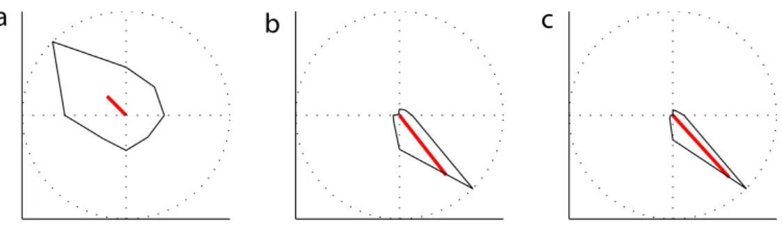
a
b
c
Figure 4: Orientation tuning curves of three neurons recorded in the primary visual cortex of an awake macaque monkey, while the monkey was watching a visual stimulus consisting of sinusoidal gratings at any of eight different orientations. Neurons were recorded extracellularly using tetrodes. Black lines indicate the orientation tuning curves of the neurons, red lines the mean resultant vectors.
6. Application to neuroscience
In this section, we provide an exemplar analysis of a set of angular data as it occurs frequently in neuroscience. Individual neurons recorded in the visual cortex of many animals show orientation tuning, i.e., they respond more vigorously to stimuli of a certain orientation. We analyze the tuning properties of three neurons recorded2 in the primary visual cortex of an awake monkey (Figure4).
The dataset consists of a vectorθ of eight orientations 0,22.5, . . . ,167.5 deg that were shown to the animal during the experiment and vectors si (i = 1,2,3) containing the number of
action potentials that were emitted by neuron i in response to a particular orientation. To subject this dataset to analysis with the methods described in this paper, we treat it as if the spikes had been binned to the presented orientations using θ as the angular variable and si
as the associated weights. Since the data is axial, we multiply each orientation by two. In Figure4, we show the responses of the three neurons as a function of orientation.
Visually, we find that all three neurons show clear orientation tuning, where neuron 4a is tuned to almost the opposite direction as neurons4b and c. Accordingly, the angular mean of neuron4a lies almost 180 deg opposite of the angular mean of the other two neurons (for an overview over descriptive measures see Table1). We confirm that the deviations from circular uniformity are highly significant for all three neurons, both when assessed with the Rayleigh test and the Omnibus test (P <10−10). Using the Watson-Williams test, we detect significant differences between the preferred orientation of the three cells (P = 0.0002, F = 12.89, 3 groups). To determine which cells have significantly different preferred orientations, we perform pairwise comparisons between cells. We find that neurons 4b and 4c dot not have significantly different preferred orientations (P = 0.339). Comparisons between the other pairs yield highly significant p-values, but violate the assumptions of the Watson-Williams test concerning the shared resultant vector length.
2This dataset has been collected for other studies of our laboratory (Tolias, Ecker, Siapas, Hoenselaar,
Keliris, and Logothetis 2007;Berenset al. 2008). A detailed description of the experimental methods used, the experimental paradigm and the background of the experiments can be found in any of these papers.
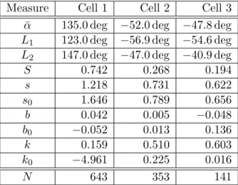
Measure Cell 1 Cell 2 Cell 3 ¯
α 135.0 deg −52.0 deg −47.8 deg L1 123.0 deg −56.9 deg −54.6 deg L2 147.0 deg −47.0 deg −40.9 deg
S 0.742 0.268 0.194 s 1.218 0.731 0.622 s0 1.646 0.789 0.656 b 0.042 0.005 −0.048 b0 −0.052 0.013 0.136 k 0.159 0.510 0.603 k0 −4.961 0.225 0.016 N 643 353 141
Table 1: Results from descriptive statistics for the three neurons studied in Section 6. Ab-breviations conform to those introduced in Section2.
Upon initial inspection, neuron4a seems to be more broadly tuned to orientation than the two other cells. As measured by the angular deviation s, neuron 4c is the most narrowly tuned cell, followed by neuron 4b. Cell 4a has almost twice the angular deviation the the two other neurons. All cells have symmetric tuning curves, with normalized skewness values b0 between 0.136 and −0.052. Neurons 4a is much less peaked than a comparable von Mises distribution as indicated by the low value of k0.
7. Conclusion
In this paper, we described theCircStat toolbox for performing statistical analysis of circular and directional data in MATLAB. The functions cover a wide range of applications from descriptive and inferential statistics. We supply the reader with parametric and nonparametric methods for testing a variety of hypothesis about circular data including testing of circular uniformity as well as one- and two-factor ANOVA testing. We believe that this toolbox will make circular statistics available to a wider range of researchers, especially in applied fields of biomedical research.
Acknowledgments
I am grateful to Marc J. Velasco for his contributions to the toolbox and a previously published report (Berens and Valesco 2009a) and Tal Krasovsky for discussions about the two-factor ANOVA. In addition, I thank Fabian Sinz, Alexander Ecker and Matthias Bethge for feedback. Andreas Tolias provided the data used in Section 6. This work has been supported by a scholarship of the German National Academic Foundation to PB and the Bernstein award by the German Ministry of Education, Science, Research and Technology to Matthias Bethge (FKZ:01GQ0601).
References
Aradottir AL, Robertson A, Moore E (1997). “Circular Statistical Analysis of Birch Colo-nization and the Directional Growth Response of Birch and Black Cottonwood in South Iceland.”Agricultural and Forest Meteorology,84(1-2), 179–186.
Batschelet E (1981). Circular Statistics in Biology. Academic Press, New York.
Berens P, Keliris GA, Ecker AS, Logothetis NK, Tolias AS (2008). “Comparing the Feature Selectivity of the Gamma-Band of the Local Field Potential and the Underlying Spiking Activity in Primate Visual Cortex.”Frontiers in Systems Neuroscience,2, 2.
Berens P, Valesco MJ (2009a). “The Circular Statistics Toolbox for MATLAB.” Techni-cal Report 184, Max Planck Institute for Biological Cybernetics. URL http://www.kyb. tuebingen.mpg.de/publication.html?publ=5873.
Berens P, Valesco MJ (2009b). CircStat2009. MATLAB toolbox, URL http://www. mathworks.com/matlabcentral/fileexchange/10676.
Boles LC, Lohmann KJ (2003). “True Navigation and Magnetic Maps in Spiny Lobsters.”
Nature,421(6918), 60–63.
Bowers JA, Morton ID, Mould GI (2000). “Directional Statistics of the Wind and Waves.”
Applied Ocean Research,22(1), 13–30.
Brunsdon C, Corcoran J (2005). “Using Circular Statistics to Analyse Time Patterns in Crime Incidence.” Computers, Environment and Urban Systems,30, 300–319.
Cochran WW, Mouritsen H, Wikelski M (2004). “Migrating Songbirds Recalibrate Their Magnetic Compass Daily from Twilight Cues.”Science,304(5669), 405–408.
Cox N (2004). CIRCSTAT: Stata Modules to Calculate Circular Statistics. URL http: //econpapers.repec.org/RePEc:boc:bocode:s362501.
Fisher NI (1995).Statistical Analysis of Circular Data. Revised edition. Cambridge University Press.
Fisher R (1953). “Dispersion on a Sphere.” Proceedings of the Royal Society of London A,
217(1130), 295–305.
Froehler MT, Duffy CJ (2002). “Cortical Neurons Encoding Path and Place: Where You Go Is Where You Are.”Science,295(5564), 2462–2465.
Gao F, Chia K, Krantz I, Nordin P, Machin D (2006). “On the Application of the von Mises Distribution and Angular Regression Methods to Investigate the Seasonality of Disease Onset.”Statistics in Medicine,25(9), 1593–1618.
Gill J, Hangartner D (2008). “Circular Data in Political Science and how to Handle it.” In
MPSA Annual National Conference. All Academic. URLhttp://www.allacademic.com/ meta/p265709_index.html.
Hanbury A (2003). “Circular Statistics Applied to Colour Images.” In Proceedings of the 8th Computer Vision Winter Workshop, pp. 55–60. URL http://allan.hanbury.eu/lib/ exe/fetch.php?media=hanbury_cvww03.pdf.
Harrison D, Kanji GK (1988). “The Development of Analysis of Variance for Circular Data.”
Journal of Applied Statistics,15(2), 197.
Harrison D, Kanji GK, Gadsden RJ (1986). “Analysis of Variance for Circular Data.”Journal of Applied Statistics,13(2), 123.
Haskey JC (1988). “The Relative Orientation of Addresses of Spouses Before Their Marriage: An Analysis of Circular Data.”Journal of Applied Statistics,15(2), 183.
Jammalamadaka SR, Sengupta A (2001). Topics in Circular Statistics. World Scientific. Kovach Computing Services (2009). Oriana for Windows. Kovach Computing Services,
Wales. Version 3, URLhttp://www.kovcomp.co.uk/oriana/.
Kubiak T, Jonas C (2007). “Applying Circular Statistics to the Analysis of Monitoring Data.”
European Journal of Psychological Assessment,23(4), 227–237.
Le CT, Liu P, Lindgren BR, Daly KA, Giebink GS (2003). “Some Statistical Methods for Investigating the Date of Birth as a Disease Indicator.” Statistics in Medicine, 22(13), 2127–2135.
Lund U, Agostinelli C (2007). CircStats: Circular Statistics. Rpackage version 0.2-3, URL
http://CRAN.R-project.org/package=CircStats.
Maldonado PE, Godecke I, Gray CM, Bonhoeffer T (1997). “Orientation Selectivity in Pin-wheel Centers in Cat Striate Cortex.”Science,276(5318), 1551–1555.
Moler C (2006). “The Growth of MATLAB and The MathWorks over Two Decades.” In
The MathWorks News & Note. The Mathworks. Accessed July 2009, URL http://www. mathworks.com/company/newsletters/news_notes/clevescorner/jan06.pdf.
Pewsey A (2004). “The Large-Sample Joint Distribution of Key Circular Statistics.”Metrika,
60(1), 25–32.
Russell GS, Levitin DJ (1995). “An Expanded Table of Probability Values for Rao’s Spacing Test.”Communications in Statistics – Simulation and Computation,24, 879–888.
Stephens MA (1969). “Multi-Sample Tests for the Fisher Distribution for Directions.”
Biometrika,56(1), 169–181.
The MathWorks, Inc (2007). MATLAB – The Language of Technical Computing, Ver-sion 2007b. The MathWorks, Inc., Natick, Massachusetts. URL http://www.mathworks. com/products/matlab/.
The MathWorks, Inc (2008). MATLAB – Statistics Toolbox, Version 7.2. The MathWorks, Inc., Natick, Massachusetts. URLhttp://www.mathworks.com/products/statistics/.
Tolias AS, Ecker AS, Siapas AG, Hoenselaar A, Keliris GA, Logothetis NK (2007). “Recording Chronically from the Same Neurons in Awake, Behaving Primates.”Journal of Neurophys-iology,98(6), 3780–3790.
van Doorn E, Dhruva B, Sreenivasan KR, Cassella V (2000). “Statistics of Wind Direction and its Increments.”Physics of Fluids,12(6), 1529–1534.
Watson GS, Williams EJ (1956). “On the Construction of Significance Tests on the Circle and the Sphere.”Biometrika,43, 344–352.
Wiltschko W, Wiltschko R (1972). “Magnetic Compass of European Robins.” Science,
176(4030), 62–64.
Zar JH (1999). Biostatistical Analysis. 4th edition. Prentice Hill.
Affiliation: Philipp Berens
Computational Vision and Neuroscience Group Max Planck Institute for Biological Cybernetics 72076 T¨ubingen, Germany
E-mail: [email protected]
URL: http://www.kyb.mpg.de/~berens/
and
Department of Neuroscience Baylor College of Medicine
Houston, TX, 77030, Unitedt States of America
Journal of Statistical Software
http://www.jstatsoft.org/published by the American Statistical Association http://www.amstat.org/
Volume 31, Issue 10 Submitted: 2009-07-27