Effective Enterprise Risk Management - Quantifying operational risks and selecting efficient risk mitigation measures

(1)

Effective Enterprise Risk Management - Quantifying

operational risks and selecting efficient risk mitigation

measures

“These days, the business of banking is risk management”

Dennis Westherstone, Retired JP Morgan Chairman

Authors:

Nils Loehndorf Executive Director, Risk Management Practice

INTERPROJECTS GmbH

Prof. Dr. Erhard Petzel CEO and Research Director ibi RESEARCH GmbH

Thomas Portmann Senior Consultant INTERPROJECTS Risk

(2)

1 Introduction

Basel II, Sarbanes-Oxley (SOX) and other similar regulatory standards have required Financial Services Institutions (FSI) to invest heavily in risk management methods, tools and processes in order to achieve the required level of compliance. Basel II is a generally accepted international framework for banks and financial institutions which promotes best practices in both risk management principles and in the measurement of regulatory capital.

The assessment of operational risk, in addition to the measurement of market risk and credit risk capital requirements, is a new item on the Basel II agenda. Capital reserves set to cover operational risk (including systems risk) will now have a direct impact on the overall capital requirements of a Bank. The corollary of this will be that rating agencies will pay more attention to capital adequacy ratios and the quality of operational risk management [Geer, D. (2004], in addition to the traditional basket of risk indicators. Although for many years, market risk and credit risk management activities impacted specialist activities (for example, traders and credit analysts) within the Bank, it is no exaggeration to say that operational risk permeates the entire enterprise, involving virtually every employee, every business process and every (ICT) system in the company.

Most of the models currently in use to quantify operational risks are based on historical loss data. Considering the constant change of technology and

organizational structures these data are not sufficient to quantify the operational risks of today.

In the following case study a more comprehensive loss distribution approach was used for work in operational risk management in a bank which had recently launched a new retail business and did not yet have a credit scoring system. The approach integrated statistical data with expert opinion and explicit modeling of risk correlations and dependencies. Based on existing business process documentation (e.g. SOX) a unified model of process, people, system and external risks was built and

parameterized by both statistical data and expert opinion. Key risk drivers (KRD) were identified and operational value at risk for these key risk drivers was calculated by using Monte-Carlo simulations. Additionally the return on investment (ROI) of specific mitigation measures was quantified. Through adopting this approach the bank could significantly improve the investment case for its risk mitigation measures and better fulfill Basel II capital adequacy requirements.

(4)

2 Business Processes and Operational Risks in Financial

Services

In the Financial Services Industry, managing risk has always been an integral part of doing business. In recent years, corporate malpractice together with an uncertain economic environment and volatile capital markets put risk management firmly into the spotlight. Banks and financial institutions focus much of their attention and investment on daily monitoring and management of market and credit risks, minimizing variability of returns and exposures.

As a consequence, IT infrastructures and services within these organizations have become more complex, due in part to the rapid growth in business (banking, e-brokerage) and restructuring of the industry (in- and outsourcing) and the ever-growing global nature of financial activities. Unquestionably, IT has been a key enabler of success in the Financial Services Industry. Few will contest the fact that this has been achieved at a price, namely the radical changes in traditional business models and methods along with all the risks that they entail. It is those risks, and in particular, operational risk, which regularly exposes the organisation to potential monetary loss. Only recently has operational risk been treated as a separate and recognized category of risk which, henceforth, will have to be managed as part of an overall corporate governance initiative.

Operational risks have often been difficult to pinpoint accurately since they have been embedded (and even lost) in the complex assessment of market and credit risk. Consider the example of unwarranted trading positions resulting from acceptances of trades from an electronic trading system. In this particular case, what should we be assessing in terms of risk? The operational risk due to the trading system (i.e., an error in acceptance rules or a programming error), the market risk due to an open trading position or a combination of both?

Clearly, for effective decisions to be made by the Board, it is of paramount

importance that the real causes and consequences of these risks be clearly identified and understood in order to manage them effectively. Furthermore, Basel II has gone some way to explicitly and formally recognize operational risk as a component of the required overall risk capital for banks and financial institutions. Basel II encourages regulatory authorities to provide incentives for large banks to implement

comprehensive risk management initiatives covering several different and overlapping groups of risks.

Regulatory requirements aside, banks and financial institutions have understood that an effective enterprise-wide system for the identification, assessment, quantification, management and monitoring of operational risk will ultimately lead to more informed business decisions and improved performance.

(5)

A study conducted by Risk Magazine in 2004 [RiskNet (2004)] on 250 financial institutions worldwide showed that:

• Basel II, SOX and other similar compliance initiatives are main drivers for the implementation of an operational risk management initiative, the most

important (expected) benefits are overall improved business performance and reductions of operational losses.

• Banks and financial institutions are looking for intelligent, judicious and cost effective implementations of compliance initiatives which contribute to business excellence and improved performance.

The Basel Committee probably provides the most commonly accepted definition of operational risk to date, as follows: Operational risk is the risk of loss resulting from inadequate or failed internal processes, people and systems or from external events. This includes legal risk but excludes strategic and reputational risk. [BIS (2003)]

Examples of operational risk include fraud either by external parties or employees, workplace safety and employment practices, client, product and business practices, damage to physical assets, business disruption and (ICT) system failures, losses from failed transaction processing or from trade with vendors. Managing operational risk can sometimes be more complex than managing market risk or credit risk. This is because it is difficult to identify and quantify operational risks when historical data is scarce and the discipline itself is relatively new, with few qualified practitioners.

(6)

3 Disadvantages of established Loss Distribution

Approaches

Taking a look at how operational risk management is currently practiced in many banks, including those with more advanced measurement approaches to optimize their models, the loss distribution approach (LDA) is “state of the art”. LDA requires the existence of ample valid loss data for sufficient past periods. Many loss data bases have been built up in the last years, trying to record extensively the high frequency, low impact operational risks and enhancing the missing data by extensive self assessments within the company or possibly using external benchmarking data. The challenges that relate to the loss distribution approaches using historical loss data are:

• Sparse existing data

• Employment of third-party loss data is impractical and partly impossible

• Past loss data may no longer reflect current state and structure of risks

• Determination of holding period problematic

• Risk prevention strategy „interferes“ with loss history

• Due to nontransparent risk drivers, VaR (Value at Risk) -levels are of little informational value to management (too aggregated, too abstract)

• Current structure / nonmaterialized risks can only be integrated by direct estimation of a new loss distribution, which is complex and difficult to reason

• Present knowledge about risk correlation cannot be formalized

In the existing loss databases one seldom finds the low frequency high-impact

operational risks that are responsible for the “fat tail” in loss distributions if one would encounter them in the data collection exercise and record them in the database.

But how many observation cycles are really needed? And if low-frequency high-impact events are included, are they statistically relevant or just a fluke? What is clear is that data and estimates really only converge over the long term (see also Figure 1 below).

(7)

Figure 1.

The above-mentioned disadvantages of the established loss distribution approaches using mainly historical data lead us to propose expanding this approach to meet the following requirements:

• Integration of statistical data with expert opinions

• Explicit modeling of risk correlations and dependencies

• Explicit consideration of corporate and process structures

• Traceable, transparent and valid quantification

• Evaluation and prioritization of risk countermeasures

It is obvious that the above requirements can only be achieved through a broader approach, embracing additional information and data. We chose a process driven approach combining simulation and scenario analysis. The idea of scenario analysis is to estimate the frequency and severity of risk events via expert opinions, taking into account bank environment factors with reference to events that have occurred (or may have occurred) in other banks. Scenario analysis is forward looking and can reflect changes in the banking environment. By itself, scenario analysis is very subjective but combined with loss data it is a powerful tool to estimate operational risk losses [Shevchenko et al; 2006]

It is important not only to quantify the operational risk capital but also to provide incentives to business units to improve their risk management policies, which can be accomplished through scenario analysis showing expected losses, value at risk and even more the direct impact of possible mitigation measures.

0 0,05 0,1 0,15 0,2 0,25 0,3 0,35 0,4 10 30 ₁₀₀ ₃₀0 100 0 3000₁₀000₃₀00 0 10000 0 30000 0 100 000 0 300 000 0 100 000 00 und gr öße r W a h rsch einli c hk eit 20 Ereignisse Anpassung no events witnessed = no risk? 5 years later: 30 events 0 0,05 0,1 0,15 0,2 0,25 0,3 0,35 0,4 10 30 100 300₁₀00 3000₁₀000 3000 0 1000 00 3000 00 1000 000 3000 000 1000 0000 und gr ößer W a h rs c h e in lic h k e it 30 Ereignisse Schätzung fluke or part of the curve? 0 0,05 0,1 0,15 0,2 0,25 0,3 0,35 0,4 10 30 ₁₀0 ₃₀0 10003000₁₀00 0 300 00 1000 00 3000 00 1000 000 300 0000 1000 000 0 und grö ßer W a hr sc he in li c h ke it 50 Ereignisse Schätzung 10 years later: 50 events Data and estimates only converge in long series

(8)

4 Case Study – Loan Application Process

Our Risk Modeling Language©1 is based on the widely accepted Business Process

Management (BPM) Methodology, and provides a problem-oriented, probabilistic framework for evaluation and quantification of risks and for computing operational value at risk for different mitigation measures. This case study shows in detail the modeling technique and the simulation approach used.

Within the project we focused on the retail banking side of the business, assessing the loan application and deposit processes in terms of operational risk exposure. We based our assessment on the process documentation we received from the bank. In order to create a viable risk model we first needed to understand the risks associated with the processes. The paradigm of our risk methodology is that all operational risks have to be understood in the framework of business processes and their

environment, so the determination of the business processes, their resources and the key risk drivers is crucial.

4.1 Operational Risk Assessment

The second main component of the risk model is the dedicated specification of risks. This includes the loss types as well as their causes. The risk modeling technique we use is a “white box approach” which takes all causes and indicators of operational risks into account (The technique is described in detail in the following chapters). So the second step was to determine all types of losses which could occur in the

relevant business process. All indicators and causes for these losses had to be specified as well. We extended our model to integrate a parallel “customer process” which made it very evident when particular risks affected customer choices in terms of further engaging with the bank or going to the competition (for example).

In order to be able to locate the occurrence of the loss events and their causes related to the business process, we worked out a questionnaire that qualified

different risk classes such as people risks, systems risks, process risks and external risks that could possibly affect this business process. That included possible kinds of risk and the reasons, conditions and influencers that possibly trigger those risks.

Questions asked related to people risks were (for example):

• Is it possible that the employees involved in the deposit application procedure commit fraud - alone or together with the borrower? For example, the head of a branch can grant a credit to a friend, the collateral is fictitious, and they share the money and disappear. Did this happen in the past? What can they do and what is the financial damage to the bank in this case? What other types of fraud are common or less common and how often do they occur? Are

1_{The Risk Modelling Language (RSL) and the Risk Simulation Engine (RSE) are copyrighted by INTERPROJECTS Risk}

(9)

there measures in order to reduce/omit such fraud or make it significantly more difficult to correct (e.g. obligatory approval of a second employee)?

• What mistakes – at which process step – can the employees possibly make? What is the consequence of each mistake (delay or recapitulation of which work steps, financial damage)? What are possible causes of such mistakes? – For example, at work step 7, the credit officer has to decide whether the

requested loan meets the requirements, in part based on his “visual

impression.” So, his wrong assessment, perhaps because of private problems or sickness, could reject a good customer; his “false positive” assessment due to friendship or misplaced trust could promote a bad customer.

Sample questions asked related to systems risks were:

• Are there IT systems used in the loan origination procedure? What damage arises if these are not available (delay or recapitulation of which work steps, financial damage)? Did this happen in the past? Are there measures in order to prevent such a default situation from arising (e.g. systems redundancy, if so, with what structure)? Can the data (perhaps all at the same time) get lost?

• Can the borrower file get lost? What happens in this case? How safely is the file stored? Are all borrower files stored in one place? What about fire / disaster which destroys the infrastructure?

Questions asked related to process risks included:

• Are there situations which handicap the deposit procedure, e.g. unavailability or insufficiency of resources like staff, workspaces, necessary external

information, or infrastructure? Did this happen in the past? Are there measures in order to rule out such a default situation? At which work step are which resources necessary to be present in detail? Are there time limits to be obeyed? Which damaging effect is expected (e.g. from delay: customers get impatient / decide to go to the competitors)?

• Are there plans to improve the loan origination process? For example: Can the use of a scoring system advance the process (perhaps because of

dispensability of work steps currently in place) in order to make it more attractive to new applicants? How does the alternative process look like? Which risks are expected to arise in case of such an improvement?

At a later stage in our assessment we quantified these aspects, including the possible financial damage and the probability of its impact. The risk management department was given a detailed questionnaire about the model parameters based on the agreements during the workshop. Beside detailed confidential information the bank provided us with the following:

(10)

• The bank has a headquarters and 29 branches.

• There are about 50 loan applications per branch and week.

• Ten of these are accepted.

• The credit amount of ten per week and over all branches is > $100,000.

• 25% of all applicants which are accepted for a loan decline the loan offer.

4.2 Key elements of the Risk Model

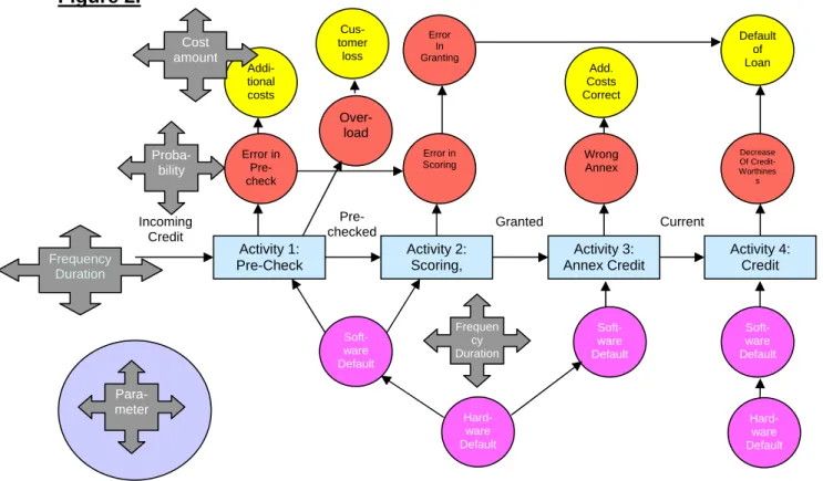
The next figure shows a graphic representation of the key elements of our risk model. The core is a standardized workflow of credit processing. The circles in dark grey and in light grey depict the process/people and system causes and the white circles show dedicated losses. Such workflows with related causes and losses are useful

templates for creating individual models for specific clients.

Figure 2. Activity 1: Pre-Check Activity 2: Scoring, Activity 3: Annex Credit Incoming Credit Soft-ware Default Soft-ware Default Hard-ware Default Activity 4: Credit Soft-ware Default Hard-ware Default Decrease Of Credit- Worthines s Default of Loan Error in Pre-check Error in Scoring Addi-tional costs Wrong Annex Error In Granting Add. Costs Correct Over-load Cus-tomer loss

Pre-checked Granted Current

Para-meter Cost amount Proba-bility Frequen cy Duration Frequency Duration

(11)

To build a computational model different parameters concerning the system

dynamics have to be obtained in expert interviews. The following list shows some of these parameters:

• Frequency of the procedure (incoming applications)

• Costs in case of loss of entire information, part of information

• Frequency of a natural calamity

• Costs in case of customer loss (escaped income)

• Probability that customer becomes impatient –and after what time?

• Probability of various errors (e.g. in scoring)

• Costs for additional work

• Frequency and duration of default of infrastructure

• Costs in case of credit default

• Probability of fraud

The following table shows the types of losses, the causes and the loss driving variables we included in the complete model.

Table 1

Types of Losses Costs of unnecessary assessment due to pre-check failure and that the applicant declines the loan offer because he becomes impatient Loss due to credit default in case of an underlying failure in applicant assessment Additional back-office operation costs due to failures

Forgone deal in case where the applicant declines the loan offer before disbursement Loss due to fraud

Types of Causes Human error in the pre-check, assessment, and back-office operation process steps Duration of the application process in conjunction with impatience of the applicant Default of the infrastructure with effect on the application process duration

Loss driving Variables

Application activity (average number of times per time unit, how often the loan application process is started)

Rate by which the application activity changes (assumed: quarterly) as effect of the market. This affects for example the variance of the loss distribution

Increased credit default probability in case of assessment failure

Loss given credit default. This and the former variable are necessary to determine the loss due to credit default in case of an underlying failure in applicant assessment

Process costs Process durations

Profit of the deal (affects the loss due to forgone deal)

Size of the deal (affects the profit, process duration and the loss given credit default). As the size of the deal affects these three other stochastical variables in

a systematic way (in the sense of a Bayesian conditioning, or statistical

correlation, resp.), the consideration of it has an increasing effect on the variance of the loss distribution

Duration of the applicant‘s patience

Fraud activity (number of times per time unit) for each competence level Levels of competence of credit granting decision

Frequency of default of infrastructure Durations of non-availability of infrastructure Human error probabilities

(12)

We did not consider the loss of information due to natural calamities / disasters. We argued that this type of loss can be omitted completely by storing the information redundantly at a different place.

4.3 Individual Risk Model

The different parameters are specifications of stochastic variables, which represent the risk associated with the tasks in the process model. In Figure 3 we highlight the Application Process.

(13)

Figure 3.

Application Processes

Start Application Process Precheck Assessment Appl. Accepted, Backoffice Operations End Application Process Applicant is waiting Duration of Patience Duration of Assessment Relative Deal Size Applicant gets impatient Applicant is gone Yes No implies Precheck Failure Costs of Unnecessary Assessment Default Due to Assessment Failure Loss Given Credit Default Loss Due to Assessment Failure Loss Due to Backoffice Operations Failure Loss Due to

Forgone Deal Profit

Duration of Backoffice Operations Process is cancelled implies enables Loss Activity of Triggering (average number of times per time unit)

Availability of Infrastructure Availability of Infrastructure Parallel branch Join Failure or applicant is already gone now?

Incidental Trigger

Duration, gamma distributed Mean: 10 working days Std.-Dev.: 7.1 working days

Relative Deal Size * Amount, exponentially distributed Mean: $15,000 Real number, gamma distributed

Mean: 1.0 Std.-Dev.: 0.71

Relative deal size * (Duration, gamma distributed Mean: 2 working days Std.-Dev.: 1.4 working days)

+ duration of infrastructure default since start of assessment + 2 working days $200 per working day Probability: 5% Probability: Appl. Accepted: 0.2% Appl. Rejected: 0% Relative Deal Size

* Amount, gamma distributed Mean: $1,500 Std.-Dev.: $1070

If default, then take input loss, else loss = $0

If applicant finally gone and no failure, then take profit as loss, else loss = $0

Sum of all losses

Amount, distributed as follows: with 0.2% prob.: $500, with 0.3% prob.: $350, otherwise, or if process cancelled: $0

Duration of infrastructure default since start of BO operations + 2 working days Disbursement of Money

(14)

The entire business process (loan application process steps and customer process) is drawn in blue. The process starts with the event “Start Application Process” and ends with the corresponding “End Application Process”. Round rectangles such as “Pre-check” and “Assessment” describe a dedicated task, an action performed at a certain point in time characterized by its duration which can be influenced by a certain variable such as “Assessment” (task) and “Duration of Assessment”

(stochastic variables). The diamond symbols within the process describe gateways, where the business process possibly branches into different threads describing parallel tasks running concurrently or exclusively depending on the dedicated process.

Because correlations exist between stochastic variables we used the concept of Bayesian Models to reflect these correlations in our model approach characterizing causal dependencies between stochastic variables with relative probability in their outcome. We modeled the interdependencies of stochastic variables such as “relative deal size”, “duration of assessment”, “loss given default” and “profit” because there is a positive correlation between “duration” and “profit” to “relative deal size” that has to be integrated into the model. In a Bayesian approach the distinction between random variables and model parameters is artificial [Peters et al; 2006], and all quantities have an associated probability distribution, representing a degree of plausibility. For in-depth discussion on the details of the approach see, for example, [Bernardo et al. 2004].

The Bayesian paradigm is a widely accepted means to implement a modern statistic-cal data analysis involving the distributional estimation of unknown “parameters”, from a set of observations. In operational risk, the observations could be both related to the losses (e.g. counts of loss events, loss amounts or annual loss amounts in dollars) and related to their indicators and causes (e.g. process durations and other quantities which are specific to the observed process instance, or number of human errors, educational degree and state of health of the personnel)

Prior knowledge of the system being modeled can be formulated through a prior distribution. In operational risk this would involve prior information collection from subject matter experts through surveys and workshops [Peters et al.; 2006], as we described in the previous chapter. The likelihood that the risks will occur may be derived from the mathematical model approximating the observed physical

phenomena, thereby relating the parameters to the observed data. In the context of operational risk this reflects the quantitative team’s modeling assumptions, such as the class of severity and frequency distributions representing the loss data

(15)

The prior distributions and likelihood are then combined through Bayes’ rule [Bayes, 1763]

to give the posterior probability of the parameters having observed the data and elicited expert opinion. The posterior probability may then be used for purposes of prediction. In this manner the Bayesian approach naturally provides a sound and robust approach to combining actual loss data observations and subject matter expert opinions and judgments [Peters et al; (2006) ]. Much literature has been devoted to understanding how to sensibly assign prior probability distributions and their interpretation in varying contexts. There are many useful texts on Bayesian inference – for further details see e.g. [Box et al. (1992) ; Gelman et al.(1995); Robert, (2004)].

4.4 Model Computation and Results

The model computation was done by a Monte-Carlo method using our own Risk Simulation Engine©. The entire risk model was simulated for one year (the reference time interval).

During this reference interval, each time a value of a stochastic variable was needed, it was generated by the random number generator included in the Risk Simulation Engine© according to the given distribution function and the current parameters. The variable under consideration (i.e. the total loss occurring during one year) was recorded. That then represented one Monte-Carlo scenario.

For the described model and for each variation (see 4.4.1 Computational Results), this was done 10,000 times. The outcome is 10,000 values for the total loss, which are used as supporting points for an interpolation which is interpreted as the loss distribution.

4.4.1 Computational Results

For the original model and each variation there is one loss distribution together with some statistical characteristics of it as the expected value, standard deviation, the 99% quantile and the value at risk.

∫

=

'

d

)

'

Pr(

)

'

|

Pr(

)

Pr(

)

|

Pr(

)

|

Pr(

θ

y

(16)

Expected Loss $12.800.000 Std.-Dev. $3.900.000 99%-Quantile $23.700.000 Value@Risk $10.900.000 Probability 0 0,25 0,5 0,75 1 0 5.000.000 10.000.000 15.000.000 20.000.000 25.000.000 30.000.000 35.000.000 Total Loss [$] Loss Density 0,0E+00 2,0E-08 4,0E-08 6,0E-08 8,0E-08 1,0E-07 1,2E-07 0 5.000.000 10.000.000 15.000.000 20.000.000 25.000.000 30.000.000 35.000.000 Total Loss [$] D e n s it y [ $ ^ -1] _ _

(17)

4.4.2 Impact of different Loss Types

We analysed each loss type separately in order to determine the proportion of the expected loss of each type with respect to the total expected loss. As the expectation value is linear, the sum of the expectations is equal to the expectation of the sum, so we may display the expected losses as a “cake chart”. In our model with its specific parameter values, the greatest part of the loss originates from the foregone deals because of impatience of the applicants.

Expected Losses $4.790.000 $275.000 $23.800 $7.690.000 $30.700

Costs of Unnecessary Assessment Loss Due to Assessment Failure Loss Due to Backoffice Operations Failure

Loss Due to Forgone Deal Loss Due to Fraud

4.4.3 Risk Mitigation Measures

The figures above show very clearly the impact of the loss types analyzed (Table 1, page 11). Based on that impact simulation (expected, unexpected loss, 99%

Quantile, Value at Risk) of the analyzed loss types it is even more important, from a business perspective, to look at possible mitigation measures to possibly reduce the effects of these losses.

We introduced three dedicated mitigation measures to the risk model to simulate their influence on the total loss distribution and the value at risk of the retail banking loan application process:

• Improved Infrastructure

• Modified Authority Level

(18)

The figures below show the simulation output pertaining to the mitigation measures listed above: 0 0,25 0,5 0,75 1 0 5.000.000 10.000.00 0 15.000.00 0 20.000.00 0 25.000.00 0 30.000.00 0 35.000.00 0 Total Loss [$] Original Model Improved Infrastructure Decreased Competence Level Optimised Process 0,0E+00 2,0E-08 4,0E-08 6,0E-08 8,0E-08 1,0E-07 1,2E-07 1,4E-07 1,6E-07 0 5.000.00 0 10.000.0 00 15.000.0 00 20.000.0 00 25.000.0 00 30.000.0 00 35.000.0 00 Total Loss [$] D e n s it y [ $ ^ -1] __ _{Original Model} Improved Infrastructure Decreased Competence Level Optimised Process

The second table shows the impact in terms of expected loss and value at risk of the chosen mitigation measures on the simulated total loss distribution of the retail banking loan application process.

Neither the improved infrastructure nor the modified authority levels have a significant impact on the total loss distribution and can thus be called a significant and valuable risk mitigation measure. In this model we halved the frequencies and the downtimes of the infrastructures. This had no “measurable” effect.2_{This is no surprise, because} the system defaults occur rarely, and if they occur, the downtime is 0.5—1.0 day.

2

Of course, we expect it to have some effect. It is not “measurable” in the sense that results from Monte-Carlo simulations are not so accurate—the precision increases proportional to the radical of the number of Monte-Carlo scenarios. So in order to see that effect, one had to compute much more MC-scenarios to increase the precision.

Black – Original Model Purple – Improved Infrastructure

Yellow – Decreased Authority Blue – Optimized Process

Black – Original Model Purple – Improved Infrastructure

Yellow – Decreased Authority Blue – Optimized Process

(19)

This cannot have an essential effect on a process whose duration is about 6 days. In terms of authority levels we modeled the impact of decreasing the highest individual authority level from $100,000 to $50,000. The effect was a negligible decrease in the expected loss over one year.

The only significant reduction of expected loss and value at risk in the retail banking loan application process could be reached by optimizing the business process in such a way as for the customer to perceive a significantly shorter waiting time until he receives a decision on his application.

With a reduction in the business process cycle time (reduction of mean duration of the loan application process by 25%) the bank then could reduce the expected loss by $ 3,630,000 and minimize the value at risk to $ 7,820,000. This amount represents the loss that would not be exceeded in a one year time frame (with a 99%

probability).

Table 2.

Scenario Figures

Scenario Expected Loss Exp. Loss Reduction Std.-Dev. 99%-Quantile Value@Risk

Original Model $12,800,000 $3,900,000 $23,700,000 $10,900,000

Improved Infrastructure $12,800,000 $0 $3,810,000 $23,500,000 $10,700,000

Decreased Authority $12,800,000 $0 $3,890,000 $23,700,000 $10,900,000

(20)

5 Operational Risk Management and Six Sigma

Recent McKinsey research [Levy, C. B.; Samandari, H (2006), page 17] suggests that saving achieved in “dedicated processes by reducing error rates (in other words, losses from operational risk) can far outweigh the savings achieved through

traditional cost reduction measures.”

Based on the experience from this case study and similar projects in other banks, we can quantify these expected loss reductions and improved value at risk by

implementing our OpRisk Performance Management Framework. Introducing these simulation results into the business decision making process on possible risk

mitigation measures can also create a better risk biased return on investment decision than the traditional cost-based approach.

The Six-Sigma method has become very popular in the light of constant business process improvement as it directly targets the possible error rate in business

processes. Statistically expressed, Six-Sigma targets an extremely low error quota of 0,00034%, which corresponds to a quality level of 99,99966%. Industry- wide the average quality level is four Sigma which means 99,4% error free products and/or processes. With a million process cycles, that means 6000 errors, and speaking revenue about 20% of total revenue [Achenbach et al. (2005), page 75].

These are process costs alone, not including the expected and unexpected losses due to operational risks that possibly outweigh the error costs. In the financial

services industry one will encounter an average of three sigma, that means an quality level in business processes of 93.3% and error costs being in amounts higher than 20% of total revenue at risk. [Achenbach et al. (2005), page 130].

So pursuing a Six Sigma strategy that includes the operational risk performance management perspective we outlined - taking the possible mitigation measures and their reduction of expected losses and value at risk into account - could radically improve the concept and outcome of change management measures to improve business processes.

Following the 20/80 rule we recommend as a business practice to focus on the 20% of business processes that have 80% of the business impact. As we have shown in our case study focussing on the retail banking application, the chosen mitigation measure of process improvement to shorten cycle time from a customer perspective has an immediate business impact in reducing the expected loss and the value at risk.

And as the authors in the McKinsey study put it “such programs also carry symbolic weight: companies that are less tolerant of their small risks are better able to control larger and less frequent ones because they create a culture of risk awareness across the organization” [Levy, C. B.; Samandari, H. (2006), page 17].

(21)

6 Summary

“Lessons are not given. They are taken” (C. Pavese)

Risk management has always been an explicit and implicit fundamental management process in financial services. In today’s world, however, there is more public attention on leading institutions, which are expected to adopt high and increasing standards to avoid things going wrong while continuing to improve corporate performance in ever changing environments. Good risk management provides a decisive competitive advantage to every bank. It helps to maintain stability and continuity and supports revenue, earnings growth and can substantially reduce cost levels, leading to better profitability.

In this article we wanted to illustrate how operational risk performance management based on business process modeling, simulation and scenario analysis can

effectively support a significant reduction of current and future risk exposure of enterprises at all operational levels. The effective use of simulation and scenario techniques can substantially enrich the loss distribution approaches already in use and stimulate better business decisions appropriate risk mitigation measures, thereby significantly reducing expected losses and value at risk that relate to dedicated

business processes and units.

The results we achieved in this and many other case studies in international financial services institutions were validated against their own internal calculations using advanced measurement approaches.

From our point of view the operational risk performance management approach we use is not limited to financial institutions calculating their capital adequacy

requirements under Basel II but extends to all industries trying to align their current and future risk exposure to their risk appetite according to their strategic business planning. As Jack Welsh, the former GE CEO, put it: “You can’t manage what you cannot measure”. Quantification of risks is in our view essential to transfer risk exposure and risk appetite into the strategic calculus of business administration to remain competitive.

(22)

References

Achenbach, W.; Lieber, K.; Moormann, J. (Hg.) (2005). Six Sigma in der Finanzbranche. Bankakademie-Verlag.

Bank for International Settlements (2003). Sound Practises for the Management of Operational Risk. http://www.bis.org/publ/bcbs.htm

Bayes, T. (1763). An essay towards solving a problem with the doctrine of Chances. Philos. Trans. R. Soc. London, 53, 370—418.

Bernardo, J.; Smith A. (1994). Bayesian Theory. Wiley Series in Probability and Statistics, Wiley.

Box and Tiao (1992) Bayesian Inference in Statistical Analysis. Wiley Classics Library.

Geer, Dan (2004). Basel II, Being Security Concious. http://www.itsecurity.com/archive/papers/stake1.htm

Gelman A., J. B. Carlin, H.S. Stern and D.B. Rubin (1995). Bayesian Data Analysis. Chapman and Hall.

Levy, C. B.; Samandari, H. (2006). Better operational-risk management for banks. McKinsey on Corporate & Investment Banking, Number 2.

Peters, G.W.; Sisson, S.A (2006). Bayesian Inference, Monte Carlo Sampling and Operational Risk, Journal of Operational Risk 1, (3).

Risk Magazine (2004). Worldwide Risk Survey, http://www.risk.net

Robert C. (2004). The Bayesian Choice, 2nd Edition. Springer Texts in Statistics.

Schevchenko, P. and M. Wuthrich (2006). The structural modelling of operational risk via Bayesian inference: Combining loss data with expert opinions. CSIRO Technical Report Series, CMIS Call Number 2371.

Effective Enterprise Risk Management - Quantifying operational risks and selecting efficient risk mitigation measures