Multiple Testing under Copula Dependency
Structures
Submitted by
André Neumann
In partial fulfillment of the requirements
for the degree of
Doktor der Naturwissenschaften
(Dr. rer. nat.)
Supervisor and referee: Prof. Dr. Thorsten Dickhaus
Second referee: Prof. Dr. Gilles Blanchard
University of Bremen, Institute for Statistics
1 Synopsis 6
1.1 Multiple testing . . . 6
1.2 Copula theory in multiple testing . . . 9
1.3 My contributions . . . 11
References . . . 13
2 Multivariate multiple test procedures based on non-parametric copula esti-mation 16 2.1 Introduction . . . 16
2.2 Oscillation behavior of Bernstein copulas . . . 18
2.2.1 Theoretical analysis . . . 18
2.2.2 The effect of smoothing . . . 22
2.3 Calibration of multivariate multiple test procedures . . . 23
2.4 Simulation study . . . 30
2.5 Real data analysis . . . 32
2.6 Discussion . . . 40
2.7 Auxiliary results . . . 42
References . . . 45
3 Estimating the proportion of true null hypotheses under arbitrary depen-dency 49 3.1 Introduction . . . 49
3.2 Estimation ofπ0via marginal parametric bootstrap . . . 53
3.3 Theoretical analysis . . . 56
3.4 Simulation study . . . 59
3.5 Real data analysis . . . 61
3.6 Discussion . . . 64
References . . . 65
Beiträge meiner Koautoren 69
Danksagung 69
Nomenclature
(e)cdf (empirical) cumulative distribution function
(p)FDR (positive) false discovery rate
ANOVA analysis of variance
FWER family-wise error rate
LFC least favorable configuration
MSE mean squared error
VaR value-at-risk
i.i.d. independent and identically distributed
w.l.o.g. without loss of generality
(Xn,F⊗n,(Pϑ⊗n, CX :ϑ∈Θ)) statistical model BK Bernstein operator BK ˆ CX,n Bernstein copula ofCX C← quantile ofu→C(u, . . .,u) CX copula of X
FXj j-th marginal cumulative distribution function ofX
H0 global null hypothesismj=1Hj
HX joint cumulative distribution function ofX
I0(ϑ) index set of true null hypotheses underϑ
K1, . . .,Km alternative hypotheses
P1, . . .,Pm p-values
E expectation with respect toP
E∗ expectation with respect toP∗
P probability measure on the elemental spaceΩor probabil-ity measure on the product spaceX∞
P∗ bootstrap probability measure
PX distribution ofX
α global significance level
αloc,1, . . ., αloc,m local significance levels T =(T1, . . .,Tm)⊤ vector of test statistics
X∗1, . . .,X∗n bootstrap resample of X1, . . .,Xn X1, . . .,Xn i.i.d. sample of X
ϕ=(ϕ1, . . ., ϕm)⊤ multiple test
ϑ parameter of interest
ϑ∗
least favorable parameter configuration
ˆ
CX,n empirical copula of X
ˆ
FXj,n j-th marginal empirical cumulative distribution function of X
ˆ
HX,n joint empirical cumulative distribution function ofX
ˆ
πSS
0 Schweder-Spjøtvoll estimator
(C([0,1]m),∥·∥∞) space of uniformly continuous functions defined on[0,1]m (ℓ∞([0,1]m),∥·∥∞) space of uniformly bounded functions on[0,1]m
C limit process ofCn
Cn empirical copula process
H={H1, . . .,Hm} set of null hypotheses
1A indicator function of the setA
π0 proportion of true null hypotheses
P
→ convergence in probability
d
→ convergence in distribution
m0 number of true null hypotheses
m1 number of false null hypotheses
n sample size o,O Landau symbols Pϑ P⊗nϑ,CX k/K k1 K1, . . ., km Km ⊤ (−∞,x] (−∞,x1] ×...× (−∞,xm] {0, . . .,K} {0, ...,K1} ×. . .× {0, . . .,Km} K k=0 K1 k1=0· · · Km km=0
1
Synopsis
The key to multiple testing is to respect the dependencies between the marginal hypothe-ses tests. Multiple tests can range from basically performing the same test multiple times to tests with very complex interactions. Any dependency structure can be modeled by so-called copula functions. This makes copulas an interesting tool in multiple testing. In particular, multivariate multiple tests explicitly utilize the dependency structure of the data. This leads to the sub-class of copula-based multiple tests.
In this synopsis, I give a general overview about multiple testing and copula theory with emphasis on their connections to my own contributions. Furthermore, I present the ideas and challenges behind my own research.
Der Schlüssel zum multiplen Testen liegt im Berücksichtigen der Abhängigkeiten zwis-chen den Randtests. Multiple Tests können dabei von einem quasi mehrfach ausge-führten Test bis hin zu komplex interagierenden Tests reichen. Jede Abhängigkeitsstruk-tur kann durch sogenannte Copula-Funktionen beschrieben werden. Dies macht Copulas zu einem interessanten Hilfsmittel im multiplen Testen. Insbesondere wird bei den mul-tivariaten multiplen Tests die Abhängigkeitsstruktur der Daten explizit verwendet. Dies führt zur Unterklasse der Copula-basierten multiplen Tests.
In meiner Synopsis gebe ich einen generellen Einblick in die Theorie der multiplen Tests und der Copulas. Die Betonung liegt dabei auf der Einordnung meiner Resultate in diese Theorien. Zudem gehe ich auf die Ideen und Herausforderungen ein, die hinter meinen Forschungsarbeiten stecken.
1.1
Multiple testing
The problem of multiple testing arises when we have to answer two or more questions considering only one data set. For example, in genetic association studies, one hypothesis is tested for every genetic marker. It is important to respect the interactions between genetic markers. Usually, these interactions are modeled as block dependency structures. Such dependency structures play a crucial role in multiple testing. In Section 1.2, we take a closer look how to model dependency structures and how to use them in multiple testing.
To clarify, a multiple test is not a simple tool to make scientific studies cheaper by testing more hypotheses on the same data. In order to successfully apply multiple testing frameworks, one should ask as few questions as possible. For a large number of hypothe-ses m, it is often helpful to reduce m. This can be achieved by applying selection or filtering methods first. Statistical learning algorithms trained on past data sets is one pos-sibility. Additionally, multiple tests for high-dimensional data can be applied. Still, model
assumptions like sparsity of the data set are necessary to achieve sufficient performance. Hence, we must carefully choose an appropriate model for each multiple test problem.
Mathematically, we test a set H = {H1, . . .,Hm} of m null hypotheses. Each null hypothesisHj is a (non-empty) subset of the parameter space Θand is tested against an alternative hypothesisKj:=Θ\Hj. For convenience and consistency, the index j denotes always a number in {1, . . .,m}. Likewise, the indexi is always in{1, . . .,n}, where nis the sample size. A multiple testϕ=(ϕ1, . . ., ϕm)⊤ :Xn→ {0,1}m
is a function on the set of data samplesXn, which maps the observed data sample x1, . . .,xnto a decision vector in{0,1}m. ϕj(x1, . . .,xn)=1means rejection of the null hypothesisHj.
It is convenient to think of multiple tests in terms of test statisticsT1, . . .,Tm, which tend to larger values under alternatives, or p-values P1, . . .,Pm, which tend to smaller values under alternatives. Thep-valuePjis basically a transformation of the test statisticTjto the uniform scale[0,1]. Such transformations are easier to interpret in terms of significance. For example, in contrast, a test statistic corresponding to the average height of some peoples is (hopefully) much smaller than a test statistic corresponding to average their income. However, this does not mean that their income is significant. Additionally, many multiple tests can be easier described in detail usingp-values. Nonetheless, test statistics are important for understanding test procedures on a general level. Sincep-values tend to smaller values under alternatives, we are interested in the boundary values of significant
p-values for which a chosen error rate is controlled. These boundary values are called the local significance levelsαloc,1, . . ., αloc,m. In the remainder, we perform multiple tests by means ofp-values and local significance levels. Therefore, ϕj(x1, . . .,xn)=1if and only ifPj =Pj(x1, . . .,xn)< αloc,j.
The most common error rates in multiple testing are the family-wise error rate
(FWER) and the false discovery rate (FDR). The FWER is older than the FDR and much stricter in terms of false rejections. A family-wise error occurs when at least one true null hypothesis is rejected. The FDR was introduced byBenjamini and Hochberg (1995) in order to relax this strict behavior and is defined as the expected proportion of false rejec-tions. This means that not too many false rejections are acceptable for each multiple test. Mathematically, we have FDRϑ(ϕ) ≤FWERϑ(ϕ)for all parameterϑ∈Θ. Therefore, the FDR is used especially for high-dimensional problems.
Classification of multiple tests
The book ofDickhaus(2014) contains a wide and well organized classification of multiple tests. Classifications are important to better understand the big picture and the starting points of my own research. In this section, we follow essentially Section 3 ofDickhaus (2014).
There are three main classes, namely marginal-based multiple tests, multivariate mul-tiple tests and closed test procedures. Marginal-based mulmul-tiple test procedures do not directly utilize the dependency structure. Instead, they work for a wide class of depen-dency structures. For example, the Bonferroni procedure (seeBonferroni(1935, 1936)) is marginal-based and one of the earliest contributions in multiple testing. The so-called Bonferroni correction sets each local significance level toαloc,j=α/m. We call it correc-tion because for each local test we correct the global significance levelα. The global level α∈ (0,1)is an upper bound for the chosen multiple test error rate and usually set to0.05 (0.01or0.1). This procedure controls the FWER and works under arbitrary dependency structures. Since this method is very easy to apply in practice, Bonferroni is still widely used.
The so-called stepwise multiple tests are contained in this class as well. The basic idea is to order the p-values and to compare each p-value Pj with a local significance level depending on the rank ofPj. For simplicity, let us just consider two examples here. The famous procedure ofBenjamini and Hochberg(1995) sets the local significance level toαloc,(j) = jα/m, where (j)denotes the index in{1, . . .,m} of the j-th smallest p-value. We search for the first p-value in descending order (say P(k)) which fails to be larger thanαloc,(k) and reject all null hypothesesH(1), . . .,H(k). This procedure controls the FDR at level m0/m·α and works under a specific class of dependency structures (see Table 5.1 in Dickhaus (2014)). Another example is the method of Holm (1979), which sets αloc,(j) = α/(m−j+1). In contrast to Benjamini and Hochberg (1995), we search for the first p-value in ascending order (again P(k)) which fails to be smaller than or equal to αloc,(k) and reject H(1), . . .,H(k−1). This procedure controls the FWER and generally improves the Bonferroni method.
Contrarily to marginal-based multiple tests, multivariate multiple test procedures ex-plicitly use the dependency structure of the data. Subclasses are resampling-based, central limit theorem based and copula-based methods. Let us just consider an example for the first subclass. The multivariate bootstrap (seeEfron(1979)) creates resamples by draw-ing from the original sample with replacement. Notice that it is important to sample with replacement. Otherwise, test statistics like the sample mean would be constant. For each resample, we evaluate the test statistics. Hence, we obtain a sample of the test statistics. This allows us to empirically calibrate the local significance levels. The bootstrap works well in one sample problems for various test statistics. In one sample problems, all ob-served data originate from the same population. In these settings, the bootstrap procedure asymptotically approximates the distribution of the test statistics. More specifically, this approximation holds almost surely or in probability with respect to the distribution of the data. In terms of copula theory, we implicitly utilize the empirical copula in this
proce-dure. This means that there are connections between resampling-based and copula-based multiple tests. We refer toWestfall and Young(1993) for an algorithm-focused book on resampling-based multiple tests.
In central limit theorem based multiple tests, the test statistics are transformations of an asymptotically normally distributed point estimator. In this way, the asymptotic distribution of the test statistics can be derived. Examples are multiple linear regression models and generalized linear models.
The emphasis of my work lies on copula-based methods. In copula-based methods, we explicitly model the dependency structure in the most general framework possible. There are two main applications. First, the FWER can be represented by the copula of the test statistics. This will be discussed further inSection 1.2. Second, we can resample from an estimated copula of the data. This falls in the category of resampling-based methods.
Closed test procedures (see Marcus et al. (1976)) cannot be exactly assigned to one of the previous two classes. Under some assumptions, we can modify existing tests and these tests can be of either class. Let us assume for now that the set of null hypothesesH contains all intersection null hypotheses. Then, a multiple testϕ′forHcan be constructed by applying the so-called closure principle on a multiple test ϕ forH. Mathematically, the testϕ′is defined byϕ′j :=minHi⊆Hjϕi. Any (coherent) testϕ with local significance level set toαloc,j =αcan be modified in this way to control the FWER at levelα. Such a modified multiple testϕ′is possibly more powerful thanϕ. Notice that we can always construct an intersection-closed setH. Hence, the main restriction is that we need local levelαtests for all intersections.
Any of the mentioned classes above could be further refined by the used error rate (FWER versus FDR) or data (low-dimensional versus high-dimensional). In my con-tributions, we consider only the FWER and low-dimensional data in the sense that the dimensionmis fixed.
1.2
Copula theory in multiple testing
The word copula means link and was introduced bySklar(1959). A copula function links the marginal cumulative distribution functions (cdfs) together to a joint cdf. Therefore, a copulaC can be seen as the dependency structure between the marginal cdfs. Mathe-matically, a copulaC:[0,1]m ⊂Rm→ [0,1]is a joint distribution function of a uniformly distributed random vector with the domain restricted to[0,1]m. This restriction is unprob-lematic because the probability mass of these random vectors is zero outside of[0,1]m. Hence, there exists a one-to-one connection between copulas and joint cdfs of uniformly distributed random vectors. Sklar’s theorem provides the relationship between the joint cdf, the marginal cdfs and the copula. This theorem is the foundation of statistical
mod-eling using copula functions.
Theorem 1.1(Sklar (1959)). Let X =(X1, . . .,Xm)⊤ be a random vector with values in
Rm and joint cdf HX. Further, let FX1, . . .,FXm denote the marginal cdfs ofX. Then there
exists a copula CX such that
HX(x)=CXFX1(x1), . . .,FXm(xm)
for allx ∈Rm. If all marginal cdfs are continuous, then the copula CX is unique.
Copula theory is focused mainly on the construction of suitable copula classes and the analysis of their structure. A standard reference for a good overview of copulas is the book ofNelsen(2006). For copula theory in the context of risk management, we refer to the books ofEmbrechts et al.(2003) andMcNeil et al.(2005).
Since we are in a more general setting, classical linear dependency structures in form of correlations are contained as well. The Gaussian copula corresponds to the correlation matrix of a normally distributed random vector. Likewise, the t-copula corresponds to the dependency structure of a (standard) multivariatet-distribution. We could of course exchange these copulas and think of marginalt-distributions combined with a Gaussian copula. In this way, new multivariate distributions can be constructed. Therefore, copulas are a very flexible and general way of modeling joint cdfs.
Some important non-parametric copulas are the empirical copula and Bernstein cop-ulas. Strictly speaking, the empirical copula fails to be continuous and therefore, is not a copula. Nonetheless, the empirical copula can be used, in particular, to construct proper copulas. Bernstein copulas are such examples. They play a crucial role in our paper Neumann et al. (forthcoming) about multiple testing based on non-parametric copula estimation (seeSection 1.3).
Connection to multiple testing
In multiple testing, we can use Sklar’s theorem to model the FWER. This enables us to think of the FWER in terms of the test statistics copula.
Lemma 1.2(Dickhaus and Gierl(2013)). Under some model assumptions, we have
FWERϑ,CX(ϕ) ≤1−CT 1−αloc,1, . . .,1−αloc,m ,
whereϑ∈Θis any parameter vector andαloc,1, . . ., αloc,mare the local significance levels. In our multiple testing setup, we are interested in an parameter vector ϑ ∈Θ corre-sponding to the marginal cdfs of the data. In this setting, the copula of the dataCX is an
infinite dimensional nuisance parameter and assumed to be independent of the parameter vectorϑ. On the other hand, the copula of the test statistics can depend on the parameter vector. Hence, the notation inLemma 1.2is somewhat imprecise. We assume that there exists a least favorable parameters configuration in the global null hypothesis mj=1Hj. The notationCT corresponds to this worst case. Often, only linear dependencies in the
form of correlations are considered in multiple testing. We are interested in what we can achieve with this more general setup.
1.3
My contributions
Multivariate multiple test procedures based on non-parametric copula estimation1 The starting point for this paper are mainly two contributions. The first one is the statis-tical analysis of the so-called Bernstein copulas in Janssen et al.(2012) and the second one is the analysis of the FWER for parametric copula models in Stange et al. (2015). In this work, we have analyzed the FWER in a semi-parametric framework. More pre-cisely, the hypotheses correspond to a finite dimensional parameter vector and the data copula is understood as an infinite dimensional nuisance parameter. The argumenta-tion is similar as in Stange et al. (2015), but dropping the continuous differentiability assumption for the quantileC←
T of the test statistics copulaCT provided some extra
chal-lenges. To clarify, by quantile of a copulaCI mean the quantile of the univariate function
u→C(u, . . .,u). An estimator ofCT← is needed in order to estimate the local significance levelsαloc,j=αloc :=1−CT←(1−α).
This makes it necessary to extend the results of the used non-parametric copula esti-mator to a suitable function space. In our theoretical analysis, we focused on Bernstein copulas. These copulas are smoothed versions of the empirical copula with Bernstein polynomials. In contrast to the empirical copula, Bernstein copulas are indeed copula functions. Our analysis is based on the results ofSegers(2012) about the empirical cop-ula in the function space of bounded functions. Previous works on Bernstein copcop-ulas in statistics have focused mainly on pointwise results for two-dimensional data (see, e.g., Janssen et al.(2012) andBelalia (2016)). Furthermore, we have extended these results to (fixed) higher dimensions m > 2. A general analysis of Bernstein copulas in higher dimensions has been done inSancetta and Satchell(2004).
In order to deduce asymptotic normality for the FWER asn→ ∞, we have proven that for the quantiles of Bernstein copulas hold pointwise asymptotic normality (at point1−α). Although this is a pointwise result, we utilize the uniform results for Bernstein copulas in the space of continuous functions. On the other hand, the consistency of the FWER
follows directly from the consistency of Bernstein copulas. The uniform consistency of Bernstein copulas is already known in two dimensions. Additionally, the argumentation is the same for fixed dimensionm>2. Hence, the core of our theoretical analysis is the asymptotic normality.
As mentioned before, we have reduced the assumptions. However, we additionally assume that the copula of the data can be transformed locally to the copula of the test statistics on the diagonal set(u, . . .,u)⊤|u∈ [0,1]. In this setting, Bernstein copulas are used to approximate only the data copulaCX. Unfortunately, this assumption is hard to verify and to exploit in practice. InBodnar and Dickhaus(2014) andStange et al.(2015), the dependency structure among the test statistics orp-values is assumed to follow a para-metric copula. Additionally, they utilize resampling methods to create an approximate sample of the test statistics (orp-values). In our paper, the strategy is similar in practice. However, we generate resamples by using a Bernstein copula of the data. After that, we calibrate the multiple test empirically. In terms of copula theory, this means that we use the empirical copula quantile of the resampledp-values for calibration.
Estimating the proportion of true null hypotheses under arbitrary dependency2 The idea for considering the proportion of true null hypotheses was to improve methods like the Benjamini-Hochberg procedure. This procedure controls the FDR at levelπ0α≤
α, where π0:=m0/m is the proportion of true null hypotheses andm0 is the number of true null hypotheses. Of course, m0 is unknown and an estimator of π0 could be used to improve this procedure such that the error rate is (approximately) controlled at level α. However, in order to avoid confusion, we focused solely on this estimation problem. Besides, it can be helpful on its own to know the value of π0. Some multiple testing methods perform better for larger (or smaller) values ofπ0than others. For example, our Bernstein procedure works better for smaller values ofπ0. To clarify, in this manuscript, we did not use the connection between multiple tests and copulas in the sense ofLemma 1.2. We have estimatedπ0only in models where the dependency structure of thep-values is modeled by copulas.
The basic estimator of π0 was introduced by Schweder and Spjøtvoll (1982). One of the assumptions for this estimator is the independence of thep-values under true null hypotheses. In multiple testing, such an assumption is often violated. There exists a vast literature on this topic but not in the context of copula theory. In the existing liter-ature, independent p-values are still often assumed or models with some specific depen-dency structures are considered. For example,Tong et al.(2013) modified the Schweder-Spjøtvoll estimator for various patterns of thep-value histogram. Implicitly, these patterns
correspond to dependency structures among thep-values.
Our initial approach was to transform the p-values utilizing the copula directly. For example, in Archimedean copula models, we constructed an algorithm based on using the sampling procedure ofWu et al.(2007) backwards. Unfortunately, this only works under very restrictive assumptions. Therefore, instead, we have constructed new p-values by utilizing a marginal parametric bootstrap algorithm. This means that we split the original data sample and apply the univariate bootstrap on every marginal sample x1,j, . . .,xn,j given the estimated parameters. More specifically, the algorithm works as follows.
Algorithm 1.3(Marginal parametric bootstrap).
1. Resample from the j-th marginal distribution function of the data given the esti-mated parameters.
2. Estimate the p-value Pjby using this Bootstrap sample.
3. Apply step 2 and 3 to every margin j and then estimate the ratioπ0.
4. Repeat the steps 2-4 B times.
5. Take the average over all B estimated values ofπ0asπˆ0.
The conditional nature (with respect to the observed data) of the bootstrap translates to the conditional independence of these bootstrap p-values. Assumptions of the bootstrap like suitable test statistics translate to our procedure as well. Additionally, we make a model assumption on the parameters for the marginal cdfs. This is necessary in order to split the sample without losing information about the parameters of interest. Fortunately, these assumptions are not hard to check.
Under a specific (mild) assumption, we have proven thatπˆ0is an consistent estimator. If the assumption is not met, then the estimator is asymptotically positively biased. In multiple testing, this could mean that procedures based on this estimator are more conser-vative than in the unbiased case.
References
Belalia, M. (2016). On the asymptotic properties of the Bernstein estimator of the multi-variate distribution function. Stat. Probab. Lett. 110, 249–256.
Benjamini, Y. and Y. Hochberg (1995). Controlling the false discovery rate: A practical and powerful approach to multiple testing. J. R. Stat. Soc., Ser. B 57(1), 289–300.
Bodnar, T. and T. Dickhaus (2014). False discovery rate control under Archimedean copula. Electron. J. Stat. 8(2), 2207–2241.
Bonferroni, C. (1936). Teoria statistica delle classi e calcolo delle probabilita.
Pubbli-cazioni del R Istituto Superiore di Scienze Economiche e Commericiali di Firenze 8,
3–62.
Bonferroni, C. E. (1935). Il calcolo delle assicurazioni su gruppi di teste. Studi in onore
del professore salvatore ortu carboni, 13–60.
Dickhaus, T. (2014). Simultaneous Statistical Inference with Applications in the Life
Sciences. Springer-Verlag Berlin Heidelberg.
Dickhaus, T. and J. Gierl (2013). Simultaneous test procedures in terms of p-value cop-ulae. InProceedings on the 2nd Annual International Conference on Computational
Mathematics, Computational Geometry & Statistics (CMCGS 2013), pp. 75–80. Global
Science and Technology Forum (GSTF).
Efron, B. (1979, jan). Bootstrap methods: Another look at the jackknife. The Annals of Statistics 7(1), 1–26.
Embrechts, P., F. Lindskog, and A. McNeil (2003). Modelling dependence with copulas and applications to risk management. In S. Rachev (Ed.), Handbook of Heavy Tailed
Distributions in Finance, pp. 329–384. Elsevier Science B.V.
Holm, S. (1979). A simple sequentially rejective multiple test procedure. Scand. J. Stat.,
Theory Appl. 6, 65–70.
Janssen, P., J. Swanepoel, and N. Veraverbeke (2012). Large sample behavior of the Bernstein copula estimator. J. Statist. Plann. Inference 142(5), 1189–1197.
Marcus, R., E. Peritz, and K. Gabriel (1976). On closed testing procedures with special reference to ordered analysis of variance. Biometrika 63, 655–660.
McNeil, A. J., R. Frey, and P. Embrechts (2005). Quantitative risk management.
Con-cepts, techniques, and tools. Princeton, NJ: Princeton University Press.
Nelsen, R. B. (2006). An introduction to copulas. 2nd ed. Springer Series in Statistics. New York, NY: Springer.
Neumann, A., T. Bodnar, and T. Dickhaus (preprint). Estimating the proportion of true null hypotheses under copula dependency. Stockholm University Research Report 2017.
Neumann, A., T. Bodnar, D. Pfeifer, and T. Dickhaus (forthcoming). Multivariate multiple test procedures based on nonparametric copula estimation. Biometrical Journal.
Sancetta, A. and S. Satchell (2004). The bernstein copula and its applications to modeling and approximations of multivariate distributions. Econometric Theory 20(03), 535– 562.
Schweder, T. and E. Spjøtvoll (1982). Plots ofP-values to evaluate many tests simultane-ously. Biometrika 69, 493–502.
Segers, J. (2012). Asymptotics of empirical copula processes under non-restrictive smoothness assumptions. Bernoulli 18(3), 764–782.
Sklar, M. (1959). Fonctions de répartition à n dimensions et leurs marges. Publ. Inst. Statist. Univ. Paris 8, 229–231.
Stange, J., T. Bodnar, and T. Dickhaus (2015). Uncertainty quantification for the family-wise error rate in multivariate copula models. AStA Adv. Stat. Anal. 99(3), 281–310.
Tong, T., Z. Feng, J. S. Hilton, and H. Zhao (2013). Estimating the proportion of true null hypotheses using the pattern of observedp-values. J. Appl. Stat. 40(9), 1949–1964.
Westfall, P. H. and S. S. Young (1993). Resampling-based multiple testing: examples
and methods for p-value adjustment. Wiley Series in Probability and Mathematical
Statistics, Applied Probability and Statistics, Wiley, New York.
Wu, F., E. Valdez, and M. Sherris (2007). Simulating from exchangeable Archimedean copulas. Commun. Stat., Simulation Comput. 36(5), 1019–1034.
2
Multivariate multiple test procedures based on
non-parametric copula estimation
André Neumann1, Taras Bodnar2, Dietmar Pfeifer3, and Thorsten Dickhaus1
Multivariate multiple test procedures have received growing attention recently. This is due to the fact that data generated by modern applications typically are high-dimensional, but possess pronounced dependencies due to the technical mechanisms involved in the experiments. Hence, it is possible and often necessary to exploit these dependencies in order to achieve reasonable power. In the present paper, we express dependency structures in the most general manner, namely, by means of copula func-tions. One class of non-parametric copula estimators is constituted by Bernstein copu-las. We extend previous statistical results regarding bivariate Bernstein copulas to the multivariate case and study their impact on multiple tests. In particular, we utilize them to derive asymptotic confidence regions for the FWER of multiple test procedures which are empirically calibrated by making use of Bernstein copulas approximations of the de-pendency structure among the test statistics. This extends a similar approach by Stange et al. (2015) in the parametric case. A simulation study quantifies the gain in FWER level exhaustion and, consequently, power which can be achieved by exploiting the de-pendencies, in comparison with common threshold calibrations like the Bonferroni or Šidák corrections. Finally, we demonstrate an application of the proposed methodology to real-life data from insurance.
Key words: Asymptotic oscillation behavior; Family-wise error rate; p-Value; Risk management
2.1
Introduction
Copula-based modeling of dependency structures has become a standard tool in applied multivariate statistics and quantitative risk management (see, e.g., Nelsen (2006), Joe (2014), Härdle and Okhrin (2010), Embrechts et al. (2003), and Chapter 5 of McNeil et al.(2005)). The estimation of an unknown copula is key to a variety of modern mul-tivariate statistical methods. In particular, applications of copulas to the calibration and the analysis of multiple tests have been considered byDickhaus and Gierl(2013),Bodnar and Dickhaus(2014), Stange et al.(2015), Cerqueti et al.(2012), Schmidt et al.(2014),
1Institute for Statistics, University of Bremen, Bibliothekstraße 1, D-28359 Bremen, Germany.
2Department of Mathematics, Stockholm University, Roslagsvägen 101, SE-10691 Stockholm, Sweden. 3Institute of Mathematics, Carl von Ossietzky University of Oldenburg, D-26111 Oldenburg, Germany.
andSchmidt et al. (2015); see also Sections 2.2.4 and 4.4 ofDickhaus (2014). Specif-ically, the copula-based construction of multiple test procedures developed byDickhaus and Gierl (2013) and Stange et al. (2015) under parametric assumptions regarding the type of dependencies among test statistics considerably extends previous approaches as inHothorn et al.(2008) which are confined to asymptotic Gaussianity and, consequently, linear dependencies.
In the case of a parametric copula, generic estimation techniques like the (generalized) method of moments or maximum likelihood estimation are established notions (cf. Sec-tion 3.2 ofStange et al.(2015) and references therein). The empirical copula as well as its asymptotic properties as a non-parametric estimator have been studied, among others, by Rüschendorf(1976),Deheuvels(1979), Stute(1984), and, more recently, byBücher and Dette(2010), andBouzebda and Zari(2013), to mention only a few references. However, similarly as multivariate histogram estimators, the empirical copula in dimensionmhas some undesirable properties. For example, it is discontinuous, and it typically assigns zero mass to large subsets of[0,1]m, even if the sample sizenis large, due to the concen-tration of measures phenomenon. One way to tackle these issues consists of smoothing of the empirical copula. In particular,Sancetta and Satchell(2004) proposed smoothing by Bernstein polynomials, leading to so-called Bernstein copulas. Approximation theory for Bernstein copulas has been derived byCottin and Pfeifer(2014), and asymptotic sta-tistical properties of Bernstein copula estimators in the bivariate case (m=2) have been proven by Janssen et al. (2012) and Belalia (2016). Functional central limit theorems for empirical copula processes have been established bySegers(2012). Applications of Bernstein copulas to modeling dependencies in non-life insurance have been considered byDiers et al.(2012).
In the present work, we contribute to theory and applications of Bernstein copulas in the case of a general dimension m ≥ 2. In Section 2.2, we extend the asymptotic theory regarding Bernstein copula estimators by proving its rate of convergence in infinity norm as well as its asymptotic normality in a function space, for arbitrary m. Also, we provide some justifications for the proposed smoothing approach. Section 2.3 is then devoted to applications of Bernstein copulas for multiple test procedures with control of the FWER, avoiding restrictive parametric dependency assumptions. The application of the central limit theorem derived inSection 2.2allows for a precise quantification of the uncertainty about the realized FWER in the case that the copula of test statistics is pre-estimated prior to calibrating the significance thresholds of the multiple test procedure. This extends the results ofStange et al.(2015) to the case of non-parametric copula pre-estimation. Section 2.4demonstrates by means of a simulation study that the latter pre-estimation approach leads to a better exhaustion of the FWER level and thus enhances the
power of the multiple test procedure compared with traditional approaches which only take univariate marginal distributions of test statistics into account. Finally, we apply the proposed multiple testing methodology to real-life data from insurance inSection 2.5, and we conclude with a discussion inSection 2.6. Lengthy proofs and some auxiliary results are deferred toSection 2.7.
2.2
Oscillation behavior of Bernstein copulas
In this section, asymptotic properties of (empirical) Bernstein copulas are studied. The main properties of Bernstein estimators are consistency (Theorem 2.1) and asymptotic normality (Theorem 2.4). The auxiliary lemmas can be found inSection 2.7. Nonetheless, the argumentation in this section is illustrated in some mathematical detail. More practi-cally oriented readers might findSection 2.2.2and the following sections more valuable. InSection 2.3, the methodology how to use this estimator in multiple testing is discussed and examples are given. The consistency of the realized FWER can be derived directly from the consistency of the Bernstein estimator. The asymptotic normality of the realized FWER follows indirectly from the asymptotic normality of the Bernstein estimator via Lemma 2.18.
Let X = (X1, . . .,Xm)⊤ be a random vector taking values in the probability space
(X,F,PX), where X ⊆ Rm, F is a σ-field over X, and PX denotes the (joint)
distribu-tion of X. The univariate marginal cdfs of X we denote byFXj, 1≤ j ≤ m, whereasCX stands for the copula related to the distributionPX.
Assume thatX1, . . .,Xnare stochastically independent and identically distributed (i.i.d.) random vectors with X1 ∼ PX. Then, the marginal empirical cumulative distribution
function (ecdf) FˆXj,n of X1,j, . . .,Xn,j ⊤ is given by FˆXj,n xj := 1 n n i=11(−∞,xj] Xi,j,
1≤ j ≤ m, and the joint ecdf is defined as HˆX,n(x):= 1nni=11(−∞,x](Xi). The symbol
1A denotes the indicator function of setA and (−∞,x]=(−∞,x1] ×...× (−∞,xm]. We will use an analogous bold-face notation for vectors throughout the remainder. Finally, the empirical copulaCˆX,npertaining to X1, . . .,Xnis given by
ˆ CX,n(u)=HˆX,n ˆ FX← 1,n(u1), . . ., ˆ FX← m,n(um) , u∈ [0,1]m. In this,FˆX←
j,ndenotes the generalized inverse of the marginal ecdf in coordinate1≤ j≤m.
2.2.1 Theoretical analysis
Denote the space of bounded functions on [0,1]m, equipped with the supremum norm, by(ℓ∞([0,1]m),∥·∥∞), and the space of continuous (and bounded) functions defined on
[0,1]m by(C([0,1]m),∥·∥∞), where ∥·∥∞ again denotes the supremum norm. The Bern-stein copula estimation is based on the BernBern-stein polynomial approximation, which for a fixed copulaCX is given by the operator BK :(ℓ∞([0,1]m),∥·∥∞) → (C([0,1]m),∥·∥∞) defined by BK(f) (u):= K k=0 f(k/K) m j=1 Pkj,Kj uj
evaluated at the function f =CX, whereKk=0:=Kk1
1=0· · · Km km=0, k/K:= k1 K1, . . ., km Km ⊤ , Pk,K(u):= K k uk(1−u)K−k,
andK1, . . .,Km are given positive integers. The Bernstein copula estimator forCX is then
defined byBK ˆ CX,n .
It is well known that continuous functions can be approximated using Bernstein poly-nomials. There are results on the convergence rate for continuous functions with bounded variation as well (see Chêng (1983)). For the special case of copula functions, it has been proved in Corollary 3.1 ofCottin and Pfeifer(2014) that any copula function can be approximated uniformly using Bernstein polynomials.
Theorem 2.1establishes the consistency rate of Bernstein copula estimators for any copula functionCX. This result is known for the bivariate case (see Theorem 1 inJanssen
et al.(2012)).
Theorem 2.1(Chung-Smirnov consistency rate). Let m be fixed. If K =K(n)is such thatmj=1K−j1/2=On−1/2(log logn)1/2, then it holds that
BK ˆ CX,n −CX ∞=O
n−1/2(log logn)1/2 almost surely, where∥g∥∞:=supu∈[0,1]m|g(u)|forg:[0,1]m−→R.
Proof. The proof can be done analogously to the proof of the bivariate case considered in
Janssen et al.(2012). By the triangle inequality we split the convergence of the Bernstein copula estimators into an inner and outer convergence. It holds that
BK ˆ CX,n −CX ∞ ≤ BK ˆ CX,n −BK(CX) ∞+ ∥BK(CX) −CX∥∞. (2.1) For the outer convergence, we get fromLemma 2.17and our assumption that
∥BK(CX) −CX∥∞=O
n−1/2(log logn)1/2.
in(2.1), we get BK ˆ CX,n −BK(CX) ∞≤ sup u∈[0,1]m K k=0 CˆX,n(k/K) −CX(k/K) m j=1 Pkj,Kj uj ≤ max k∈{0,...,K} CˆX,n(k/K) −CX(k/K) ,
where{0, . . .,K}:={0, ...,K1} ×. . .× {0, . . .,Km}. LetU1, . . .,Un be a sample of random vectors defined byUi,j:=Fj
Xi,j
,1≤i≤ n,1≤ j ≤m. Application of the identity (see, e.g., Section 3 of Swanepoel(1986)) FˆU←
j,n uj = FXj ˆ FX← j,n uj leads toCˆX,n(k/K)= ˆ HU,n ˆ FU← 1,n k1 K1 , . . .,Fˆ← Um,n km Km and BK ˆ CX,n −BK(CX) ∞ ≤ max k∈{0,...,K} CˆX,n(k/K) −CX(k/K) ≤ max k∈{0,...,K} ˆ CX,n(k/K) −CX ˆ FU← 1,n k1 K1 , . . .,Fˆ← Um,n km Km (2.2) + m j=1 max kj∈{0,...,Kj} ˆ FU← j,n k j Kj − kj Kj . (2.3)
From Theorem 2 ofKiefer(1961), we get that the summand in (2.2) is of orderO
n−1/2
(log logn)1/2 as well as that each summand in (2.3) is of orderO
n−1/2(log logn)1/2.
This completes the proof.
Remark2.2. Ifmis not fixed, then the convergence rate in the last step of previous proof changes toO
mn−1/2(log logn)1/2
. Hence, we get almost surely
BK ˆ CX,n −CX ∞=O mn−1/2(log logn)1/2 .
The next theorem is taken from Whitt (2002) and will be useful in order to show asymptotic normality of Bernstein copula estimators.
Theorem 2.3(Generalized Continuous Mapping Theorem). Let g and gn, n≥ 1, be
measurable functions mapping(S,d)into(S′,d′). Let the range(S′,d′)be separable. Fur-ther, let E be the set of x in S such thatgn(xn) →g(x)fails for some sequence{xn:n≥1}
with xn→x in S. If Xn d
→X, n→ ∞, in(S,d)(→d denotes the convergence in distribution) andP[X ∈E]=0, thengn(Xn)
d
→g(X), n→ ∞, in(S′,d′).
Furthermore, we need a result for the convergence of the empirical copula process Cn:=n1/2
ˆ
CX,n−CX
Gaus-sian process with (almost surely) continuous paths and covariance function given by
Cov(γ(u), γ(v))=CX(u∧v) −CX(u)CX(v)
for allu,v∈ [0,1]m. Denoteγjuj :=γ1, . . .,1,uj,1, . . .,1. Then under some assump-tions, the processC(u):=γ(u) −mj=1∂jCX(u)γjuj is the weak limit of the empirical copula processCn in (ℓ∞([0,1]m),∥·∥∞) as shown in Proposition 3.1 of Segers (2012). With these two arguments we can proof a functional central limit theorem for Bernstein copula estimators.
Theorem 2.4(Asymptotic normality). Let m be fixed. Assume that the first order partial derivatives of CX exist and are continuous. IfK =K(n)is such that n1/2mj=1K−j1/2→0,
n→ ∞, then it holds that
n1/2·BK ˆ CX,n −CX d −→Cas n→ ∞ in(C([0,1]m),∥·∥∞).
Remark 2.5. The assumption of the existence and continuity of the first order partial
derivatives on the boundaries can be weakened (see Condition 2.1 ofSegers(2012)).
Proof. We split the Bernstein copula processn1/2·BK
ˆ CX,n −CX
into two parts. We get n1/2·BK ˆ CX,n −CX =BK n1/2 ˆ CX,n−CX +n1/2(BK(CX) −CX) =BK(Cn)+n1/2(BK(CX) −CX).
The second summand converges uniformly to zero because ofLemma 2.17and our as-sumptions. The first summand is the empirical copula processCntransformed by a family of operatorsBK, whereK =K(n).
We will use the Generalized Continuous MappingTheorem 2.3. Let(S,d):=
(ℓ∞([0,1]m),∥·∥∞) and (S′,d′) := (C([0,1]m),∥·∥∞). Then (S′,d′) is a separable space, since the set of polynomials on [0,1]m with rational coefficients is a countable dense subset of S′. Further, let gn : S → S′ be defined by gn := BK(n) and g : S → S′ be the identity function on S′ and arbitrary on S\S′. Notice that it does not matter, how g is defined on S\S′, since we are interested in g(C) and without loss of generality (w.l.o.g.) C takes values in S′ (see Section 3 of Segers (2012)). Let E be the set of
f in S such that gn(fn) →g(f) fails for some sequence {fn:n≥1} with fn→ f in S. Then E ⊆ S\S′, since we can choose fn:= f for f ∈ S′ and get uniform convergence
by Bernstein’s theorem (or by using Corollary 3.1 ofCottin and Pfeifer(2014)). Hence, P[C∈E] ≤P[C∈S\S′]=0.
The last thing we need to check is the weak convergence of the empirical copula processCnto Cin(ℓ∞([0,1]m),∥·∥∞). As already mentioned, Segers(2012) has shown this convergence under assumptions only regarding the first order partial derivatives of
CX. Therefore, the proof is complete by using Proposition 3.1 ofSegers(2012) and the
generalized continuous mapping theorem.
This result extends the pointwise central limit theorems of Janssen et al.(2012) and Belalia(2016) and works under weaker assumptions as well.
2.2.2 The effect of smoothing
This section is meant to be an addition to the simulation study ofOmelka et al. (2009). Conducting such an extensive study ourselves would go beyond the scope of this paper. Nevertheless, it is an important question how precise the Bernstein estimator is compared to other copula estimators, and this should be discussed at least to some extent.
There exists a wide variety of methods to estimate copula functions non-parametric-ally. Usually, the empirical copula or some sort of smoothing method is used. Bernstein estimators studied inSection 2.2.1are only one specific smoothing method among many others. Further examples comprise kernel (density) estimators (see Gijbels and Miel-niczuk(1990)), and beta density estimators (seeChen(1999)). It is beyond the scope of the present work to compare all these competing approaches in detail. Generally speak-ing, the empirical copula is robust and universal, but it is not a copula in the strict sense, because it lacks continuity and does not have uniform margins. Bernstein copulas are differentiable estimators, but they converge rather slowly and cannot capture extreme tail dependencies (seeSancetta and Satchell (2004)). Recently, families of non-parametric copula estimators capable of modeling (positive) tail dependence have been studied by Pfeifer et al.(2017). Kernel methods suffer from a boundary bias, although several mod-ifications like the mirror approach bySchuster(1985) exist to address this problem. Beta density estimators avoid the boundary bias, but the choice of their smoothing parameter is not trivial.
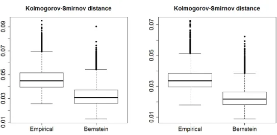
Let us briefly provide some numerical justifications for smoothing of the empirical copula. In Section 3 ofOmelka et al.(2009) some kernel methods have been compared in simulations under two prototypical models (Model 1 and Model 2). In Model 1, the data follow a Frank copula with parameter corresponding to Kendall’sτ=0.25. In Model 2, a Clayton copula corresponding to Kendall’sτ=0.75is used.
We have applied our proposed Bernstein estimator to these models as well. Figure 1 displays the results of a simulation study under these two models. The box plots
demon-Figure 1: Comparison of the Bernstein copula and the empirical copula in the setting of Model 1 (left) and Model 2 (right) ofOmelka et al.(2009) with respect to the supremum norm (Kolmogorov-Smirnov distance).
strate that the estimation accuracy (measured in terms of the Kolmogorov-Smirnov dis-tance) can be improved by smoothing. Here, we only considered smoothing by means of Bernstein polynomials, but the simulation results for various kernel methods presented by Omelka et al.(2009) are very similar. Hence, in practice it may not be most important which smoothing method to choose, while it is recommendable to smooth at all. For a more detailed overview on copula estimation methods, seeCharpentier et al.(2007).
2.3
Calibration of multivariate multiple test procedures
In this section, we assume that we have uncertainty about the distribution ofX. We thus consider a statistical model of the form(X,F,(Pϑ,CX :ϑ ∈Θ,CX ∈ C)). The probability measurePϑ,CX is indexed by two parameters. The parameterCX denotes the copula ofX,
andϑ is a vector of marginal parameters which refer to FX1, . . .,FXm. The model for the i.i.d. sampleX1, . . .,Xnconsequently reads as(Xn,F⊗n,(P⊗nϑ,CX :ϑ∈Θ,CX ∈ C)).
Based on this model, we consider multiple test problems of the form(Xn,F⊗n,(
P⊗nϑ,CX:
ϑ∈Θ,CX ∈ C),H ), where H ={H1, . . .,Hm} with∅, Hj ⊂Θfor all1≤ j ≤m denotes a family ofmnull hypotheses regarding the parameterϑ. For notational convenience, we will writePϑ,CX forP
⊗n
ϑ,CX. The copulaCX is not the primary target of statistical inference,
but a nuisance parameter in the sense that it does not depend on ϑ. This is a common setup in multiple test theory. We will mainly consider a semi-parametric situation, where Θis of finite dimension, whileCis a function space.
Remark2.6. The assumption that the number of tests equals the dimension of X is only
with obvious modifications.
A multiple test for a given set of hypothesesH is a measurable mappingϕ=(ϕ1, . . .,
ϕm)⊤:Xn→ {0,1}m, whereϕj(x1, . . .,xn)=1for given datax1, . . .,xnmeans rejection of the j-th null hypothesisHj in favor of the alternative Kj=Θ\Hj,1≤ j ≤m. We restrict our attention to multiple testsϕwhich are such that the hypotheses are rejected if the re-spective test statistics are large enough for given data, i.e., larger than their corresponding critical values. Notationally, this mean that
ϕj=1(cj,∞)(Tj), 1≤ j ≤m, (2.4) whereT =(T1, . . .,Tm)⊤:Xn→Rm denotes a vector of real-valued test statistics which tend to larger values under alternatives, andc=(c1, . . .,cm)⊤ are the critical values. In many problems of practical interest, Tj will only use the marginal data (xi,j)1≤i≤n, for every1≤ j ≤m. For example, this typically holds true ifϑjonly corresponds toFXj, and
Hj only concernsϑj, for every1≤ j ≤m.
For the calibration ofc, we aim at controlling the FWER in the strong sense. Strictly speaking, our procedure will only control the FWER under the global null hypothesis in the first place. However, strong control follows directly underAssumption 2.7(a). For sufficient conditions of this assumption seeLemma 2.8.
For givenϑ∈ΘandCX ∈ C, the FWER is defined as the probability for at least one false rejection (type I error) ofϕunderPϑ,CX, i.e.,
FWERϑ,CX(ϕ)=Pϑ,CX j∈I0(ϑ) ϕ j=1 ,
whereI0(ϑ)={1≤ j ≤m:ϑ∈Hj} denotes the index set of true null hypotheses under ϑ. The multiple testϕis said to control the FWER at levelα∈ [0,1], if
sup
ϑ∈Θ,CX∈C
FWERϑ,CX(ϕ) ≤α.
Notice that, although the trueness of the null hypotheses is determined byϑ alone, the FWER depends on ϑ and CX, because the dependency structure in the data typically
influences the distribution ofϕwhen regarded as a statistic with values in{0,1}m.
Throughout the remainder, we assume that the following set of conditions is fulfilled.
Assumption 2.7.
favorable configuration (LFC)ϑ∗∈H0such that
∀ϑ∈Θ∀CX ∈ C:FWERϑ,CX(ϕ) ≤FWERϑ∗,
CX(ϕ).
If this assumption is fulfilled, then weak FWER control implies strong FWER con-trol. Notice that this assumption can be weakened by considering closed test proce-dures, where our proposed methodology is applied to every non-empty intersection hypothesis inH (cf. Remark 1 ofStange et al.(2016) for details). However, in such a setting, the computation time for the multiple test can increase very fast with the number of hypotheses.
(b) The vector of marginal cdfs of T = (T1, . . .,Tm)⊤ depends on ϑ only, and is (at
least asymptotically as n→ ∞) known under any LFCϑ∗. We denote the vector of
marginal cdfs ofT =(T1, . . .,Tm)⊤under such an LFCϑ∗byFT =(FT1, . . .,FTm) ⊤.
(c) Letting CT =CT,ϑ∗ denote the copula ofT under ϑ
∗
from part (b), there exists a continuously differentiable function h : [0,1] → [0,1] such that CT(u, . . .,u) =
h(CX(u, . . .,u))for all u∈ [0,1], where CX is the copula ofX. The function h may be unknown. Notice that, if Tj only uses the data(xi,j)1≤i≤n, for every 1≤ j ≤ m,
then the copula ofT is independent ofϑ∗. The existence of h is guaranteed
when-ever plateaus of u →CX(u, . . .,u) occur on the same subset of [0,1] as plateaus of u →CT(u, . . .,u). In particular, h exists if u→CX(u, . . .,u)is strictly increas-ing. The more crucial part of the assumption is that h needs to be continuously differentiable.
The following lemma is useful in order to verify assumption (a).
Lemma 2.8. Let Hj: ϑ
∈Θϑj∈Θj ⊆R,1≤ j≤ m, such that the global null
hypoth-esis H0is not empty and let the marginal distributions of the data in coordinate j depend
onϑjonly. Further, assume that every test statistic Tj only uses the data(xi,j)1≤i≤n. Then
for allϑ ∈Θ, CX ∈ C and any multiple test ϕ which is as in (2.4), we can construct a
parameter valueϑ∗∈H0with
FWERϑ,CX(ϕ) ≤FWERϑ∗,CX(ϕ).
In particular, this implies that the LFC is located in H0.
Proof. Chooseϑ∗∈H0,∅withϑj∗=ϑj for j ∈I0(ϑ). Then it holds that
Pϑ,CX j∈I0(ϑ) Tj >cj =Pϑ∗,C X j∈I0(ϑ) Tj>cj ,
since it is assumed that the test statisticsTj, j ∈ I0(ϑ), only utilize the data from that coordinate j. Hence, FWERϑ,CX(ϕ)=Pϑ,CX j∈I0(ϑ) Tj>cj =Pϑ∗, CX j∈I0(ϑ) Tj >cj ≤Pϑ∗, CX m j=1 Tj >cj =FWERϑ∗, CX(ϕ). More generally, the previous lemma holds if the test statistics satisfy the so-called sub-set pivotality condition (seeWestfall and Young(1993) andDickhaus and Stange(2013)). Before we start to explain the proposed method for the calibration ofc, let us illustrate prototypical example applications of our general setup.
Example 2.9.
(a) LetΘ=Rm and assume thatϑj ∈Ris the expected value ofXj for every1≤ j ≤m. The j-th null hypothesis may be the one-sided null hypothesis Hj={ϑj ≤0}with corresponding alternative Kj={ϑj >0}. Assume that the variance of the marginal distribution of each Xj is known and w.l.o.g. equal to one. A suitable test statistic
Tj is then given byTj(X1, . . .,Xn)=ni=1Xi,j/
√
n. FromLemma 2.8it follows that the LFC lies inH0. Since the test statistics tend to get larger with increasing values ofϑ, the LFCϑ∗equals0. Underϑ∗, we have thatFTj =Φ(the cdf of the standard normal law on R) is the cdf of the (asymptotic) null distribution of Tj for every
1≤ j ≤m. If the considered copula familyCconsists of multivariate stable copulas (meaning that the observables follow a multivariate stable distribution), then the copulaCT is of the same type asCX, hence all parts ofAssumption 2.7are fulfilled.
(b) LetX=[0,∞)and assume that the stochastic representationsXj d
=ϑjZjwithϑj>0 hold true for all 1≤ j ≤m, where Zj is a random variable taking values in[0,1]. The parameter of interest in this problem is ϑ ∈ (0,∞)m. For each coordinate j, we consider the pair of hypotheses Hj : {ϑj ≤ ϑ∗j} versus Kj : {ϑj > ϑ∗j}, where the LFC ϑ∗ ∈ (0,∞)m (same argumentation as in (a)) is identical to the hypoth-esized upper bounds for the supports (or right end-points of the distributions) of
the Xj’s. This has applications in the context of stress testing in actuarial science and financial mathematics (cf., e.g., Longin (2000)). Suitable test statistics are given by the component-wise maxima of the observables, i.e., Tj(X1, . . .,Xn)=
max1≤i≤nXi,j/ϑ∗j,1≤ j ≤m. Assuming that the tail behavior of each Xj is known such that the marginal (limiting) extreme value distribution ofTj underϑ∗ can be derived and lettingCconsist ofmax-stable copulas, all parts ofAssumption 2.7are fulfilled here, too.
Let us remark here that these two examples have been treated under the restrictive assumption of one-parametric copula families Cby Stange et al.(2015). The following lemma is taken fromDickhaus and Gierl (2013) and connects the FWER with the test statistics copulaCT.
Lemma 2.10. LetAssumption 2.7be fulfilled. Then we have that FWERϑ,CX(ϕ) ≤1−CT 1−α(1) loc, . . .,1−α (m) loc ,
where αloc(j) = 1−FTj(cj(α)) denotes a local significance level for the j-th marginal test
problem. In practice, it is convenient to carry out the multiple test procedure in terms of p-values Pj=1−FTj(Tj)such thatϕj=1[0,α(j)
loc)
(Pj).
Proof. The assertion follows fromAssumption 2.7(a) and Sklar’s Theorem, since it holds
that FWERϑ,CX(ϕ) ≤FWERϑ∗,CX(ϕ) =1−CT FT1(c1(α)), . . .,FTm(cm(α)) =1−CT 1−αloc(1), . . .,1−αloc(m). Lemma 2.10shows that the problem of calibrating the local significance levels corre-sponding tocis equivalent to the problem of estimating the contour line ofCT at contour level1−α. Any point on that contour line defines a valid set of local significance levels. Thus, one may weight themhypotheses for importance by choosing particular points on the contour line. If allm hypotheses are equally important it is natural to choose equal local levels αloc(j) ≡ αloc for all 1 ≤ j ≤ m. This amounts to finding the point of inter-section of the contour line ofCT at contour level 1−α and the “main diagonal” in the
m-dimensional unit hypercube. Assumption 2.7(c) is tailored towards this strategy and should be modified accordingly if a different weighting scheme is used.
Recall that we assume that CX and, consequently, CT are unknown. Based on our investigations inSection 2.2and making use ofAssumption 2.7 (c), we thus propose to calibrateϕempirically. Ifhis known, this can be done by solving the equation
h BK ˆ CX,n (1−αloc, . . .,1−αloc) =1−α (2.5)
forαloc. Note that this assumption is formulated for equally important hypotheses and has to be modified for different situations. If for a givenαthe solution of(2.5)is not unique, one should choose the smallest set of local significance levels such that(2.5) holds. We denote the solution of(2.5)byαlocˆ ,n. This leads to the representation
ˆ αloc,n=1−BK ˆ CX,n ← (h←(1−α)), whereBK ˆ CX,n ← is the quantile ofu→BK ˆ CX,n (u, . . .,u). Since BK ˆ CX,n depends on the data,αlocˆ ,nis a random variable and
FWERϑ∗,
CX(ϕ)=1−CT
1−αlocˆ ,n, . . .,1−αlocˆ ,n
is a random variable, too, which is distributed around the target FWER level α. The following theorem is the main result of this section and quantifies the uncertainty about the realized FWER if the empirical calibration ofϕis performed via(2.5).
Theorem 2.11.LetAssumption 2.7be fulfilled. Then the realized FWER has the following properties.
a) Consistency:
∀CX ∈ C:FWERϑ∗,CX(ϕ) →αalmost surely as n→ ∞.
b) Asymptotic Normality: ∀CX∈ C: √ n FWERϑ∗, CX(ϕ) −α d → N (0, σα2)as n→ ∞, where σ2 α= σ 2(C T(1−α), . . .,CT(1−α)) C′ X(CT(1−α)) 2 · CT′ (CT(1−α))2, σ2(u):=
V[C(u)], and C′X, CT′ denotes the first derivative of the univariate
c) Asymptotic Confidence Region: ∀δ ∈ (0,1)∀CX ∈ C: lim n→∞Pϑ ∗, CX √ nFWERϑ ∗, CX(ϕ) −α ˆ σn ≤ z1−δ =1−δ,
whereσˆn2:Xn→ (0,∞)is a consistent estimator of the asymptotic varianceσα2. In this, zβ=Φ−1(β)denotes the β-quantile of the standard normal distribution onR. Proof.
a) LetCX ∈ C be arbitrary, but fixed. Since his continuously differentiable,h is also Lipschitz-continuous with Lipschitz constant L>0. Therefore, with Theorem 2.1 we get FWERϑ ∗, CX(ϕ) −α = 1−α−CT 1−αlocˆ ,n, . . .,1−αlocˆ ,n = h BKCˆX,n 1−αlocˆ ,n, . . .,1−αlocˆ ,n −h CX 1−αlocˆ ,n, . . .,1−αlocˆ ,n ≤ h BK ˆ CX,n −h(CX) ∞ ≤ L· BK ˆ CX,n −CX ∞ =O
n−1/2(log logn)1/2 almost surely.
b) Lettingp:=h←(1−α),Lemma 2.18yields that √ n1−αlocˆ ,n−C←X (p) =√n BK ˆ CX,n ← (p) −C←X (p) d −→ N 0,σ 2 C← X (p), . . .,C ← X (p) C′ X C← X (p) 2 .
Therefore, applying the Delta Method tou→CT(u, . . .,u), we have that √ n FWERϑ∗,C X(ϕ) −α =−√nCT 1−αlocˆ ,n, . . .,1−αlocˆ ,n − (1−α) =−√nCT 1−αlocˆ ,n, . . .,1−αlocˆ ,n −CT C←X (p), . . .,C←X (p) d −→ N 0,σ 2 C←X (p), . . .,C←X (p) C′XC←X (p) 2 · CT′ C←X (p) 2 .
c) Sinceσnˆ →σα almost surely and particularly, in distribution forn→ ∞, the asser-tion follows directly from part b) using Slutsky’s Theorem.
If the function his unknown, one may approximate the value ofαlocˆ ,nwith high pre-cision by a Monte Carlo simulation for a given number M of Monte Carlo repetitions. To this end, generate M×n pseudo-random vectors which follow the estimated (joint) distribution of X under ϑ∗, by combining BK
ˆ
CX,n
and the marginal cdfs FX1, . . .,FXm of X1, . . .,Xm under the global null hypothesis. From these, calculate a pseudo-sample T1, . . .,TM from the distribution ofT underϑ∗. Then,FT1(T1), . . .,FTM(TM)constitutes a pseudo-random sample from the estimator ofCT, and the empirical equi-coordinate(1−
α)-quantile of this pseudo-sample approximatesαlocˆ ,n. Since the number M of pseudo-random vectors to be generated is in principle unlimited,Theorem 2.11continues to hold true if this strategy is pursued. We will make use of this approach in the more involved examples studied inSection 2.4andSection 2.5.
2.4
Simulation study
In this section we report the results of a simulation study regarding the FWER and the power of multiple tests which are empirically calibrated as proposed inSection 2.3. As-sume w.l.o.g. thatI0(ϑ):={1, ...,m0}and letm1:=m−m0. The empirical FWER is given by the relative frequency over theLsimulation runs of the occurrence of at least one false rejection, i.e., eFWER(ϕ):=L−1 L ℓ=1 1m0 j=1 ϕ(ℓ) j =1 x(1ℓ), . . .,x(nℓ) .
Likewise, the empirical power is defined as the average proportion of true rejections, i.e.,
ePower(ϕ):= L−1 L ℓ=1 © « m−11 m j=m0+1 1 ϕ(ℓ) j =1 x(1ℓ), . . .,x(nℓ) ª ® ¬ , wherex(1ℓ), . . .,x(nℓ)
∈ Xndenotes the pseudo-sample in theℓ-th simulation run.
The setting is as follows. We simulate from various one-parametric copula models (namely, Frank, Clayton, Gumbel, Student’s t with four degrees of freedom, and the product copula) with parameters corresponding to weak (Kendall’sτ≈0.25) and strong dependence (Kendall’sτ≈0.75), respectively. In the case of t4-copulas we restrict our attention to the case of equi-correlation, and the parameter is the equi-correlation coeffi-cient. For convenience (and without loss of generality), the data are marginally normally
distributed with all marginal variances equal to one. In the inference procedures, how-ever, we assume these variances to be unknown, leading to Studentized test statistics. For each1≤ j ≤ m, we let ϑj be the mean in coordinate j. In all simulation settings, ϑj is set to0.4 under alternatives. The null hypotheses are given by Hj:{ϑj =ϑ∗j =0}, with two-sided alternatives. Hence, marginal two-sidedt-tests are performed with multiplicity corrected local significance level. Our Bernstein procedure is compared with the widely used Bonferroni and Šidák methods.
Notice that Assumption 2.7 is fulfilled. From Lemma 2.8 we get that the LFC is indeedϑ∗=(0, . . .,0)⊤. Further, the marginal distribution functions of the test statistics are known (even for finiten) and the function hexists, sinceu→CX(u, . . .,u) is strictly increasing for the choices of CX in this simulation study. However, the function h is unknown in contrast to the examples inSection 2.3.
The calculation of the Bernstein copula has been performed as in Example 4.2 of Cottin and Pfeifer(2014), which usesKj :=n for all j ∈ {1, . . .,m}. This choice fulfills the assumption of Theorem 2.1. In order to meet the assumptions of Theorem 2.4 it would be necessary to chooseKj slightly larger. Notice, however, that we consider small sample sizes n ∈ {20,100} in our simulations, such that asymptotic considerations do not apply here. Instead, some preliminary simulations indicated that the choice Kj ≡
n is appropriate. The choice of n was motivated by the purpose to demonstrate how accurately the Bernstein estimator performs in a small sample scenario. For instance, the real data example that we will present inSection 2.5has a sample size ofn=20. With the simulations presented here, we can thus evaluate the appropriateness of the application of the proposed methodology in this real data example.
Since the functionhis assumed unknown here, we calibrate the proposed multiple test with the following algorithm which was outlined at the end ofSection 2.3.
Algorithm 2.12.
1. Choose a number M of Monte Carlo repetitions.
2. For each b=1, . . .,M draw a sampleU#1b, . . .,Un#bof BKCˆX,n and calculate Xi#,jb=σjˆ ·Φ−j1 Ui#,bj +ϑ∗ j, 1≤i≤n,1≤ j ≤m,
whereσjˆ is the sample standard deviation of X1,j, . . .,Xn,j.
3. For all1≤ j ≤m, compute
Tj#b=Tj X#1b, . . .,X#nb = √ n· 1 n n i=1X# b i,j −ϑ ∗ j ˆ σ#b j
and obtain the pseudo-sample
Vj#b=2Ftn−1
Tj#b−1
from the copula ofT. 4. Finally, calibrateαlocˆ ,n=
ˆ α(1) loc,n, . . .,αˆ (m) loc,n ⊤ by solving #b V #b j ≤1−αˆ (j)
loc,nfor all1≤ j ≤m
=⌈(1−α)M⌉. (2.6)
Notice that in(2.6), we implicitly weight the hypotheses. This means that the weights corresponding to the obtained αlocˆ ,n depend on the simulation data, for convenience of implementation. In comparison, the classical Bonferroni and Šidák corrected local sig-nificance levels are given by
α(j) loc = α m andα (j) loc=1− (1−α) 1/m, 1≤ j ≤m, respectively.
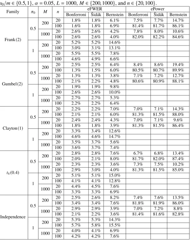
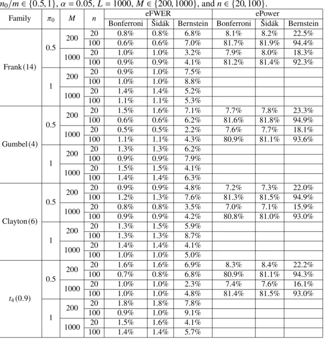
The results are displayed inTable 1(weak dependence with Kendall’sτ≈0.25) and Table 2(strong dependence with Kendall’sτ≈0.75). They reveal that in this simulation study the Bernstein method performs best in the case thatMis large and the proportion of true null hypothesesπ0 is not too large, i.e., in these cases its empirical FWER is closer toαand its empirical power is higher than those of the generic calibrations. Under strong dependence the power of the Bernstein method increases even further. On the other hand, if all hypotheses are true then the empirical FWER for the Bernstein method can be above α=5%and M needs to be large in order to improve the empirical FWER. Surprisingly, the sample sizendoes not have a clear positive impact in this simulation study.
2.5
Real data analysis
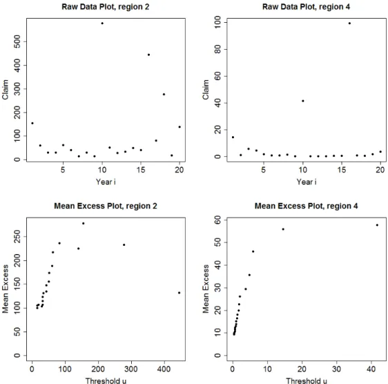
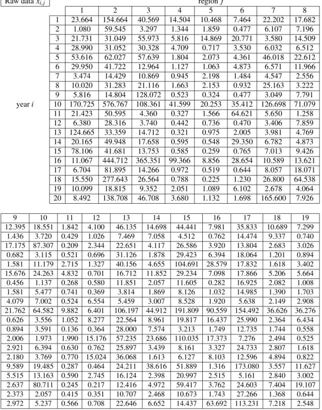
In this section, we analyze insurance claim data fromm=19 adjacent geographical re-gions (seeTable 5). For every region j ∈ {1, . . .,19}these claims have, for confidentiality reasons, been adjusted to a neutral monetary scale. The claim amounts and types have been aggregated to full years, such that temporal dependencies are considered negligi-ble. However, strong non-linear spatial dependencies are likely to be present in the data. Hence, we treat each of then=20rows inTable 5as an independent repetition Xi= xi of anm-dimensional random vectorX =(X1, . . .,Xm)⊤, where1≤i≤20is the time index in years andm=19refers to the regions.
Table 1: Comparison of empirical FWER and power regarding Bonferroni, Šidák and Bernstein corrections under various weak dependency structures with m = 20, π0 =
m0/m∈ {0.5,1},α=0.05, L=1000, M ∈ {200,1000}, andn∈ {20,100}.
Family π0 M n eFWER ePower
Bonferroni Šidák Bernstein Bonferroni Šidák Bernstein
Frank(2) 0.5 200 20 1.8% 1.8% 6.1% 7.5% 7.7% 14.7% 100 1.6% 1.8% 6.9% 81.4% 81.7% 86.1% 1000 20 2.6% 2.6% 4.2% 7.8% 8.0% 10.6% 100 2.6% 2.6% 4.0% 82.0% 82.2% 84.6% 1 200 20 5.2% 5.2% 14.6% 100 3.0% 3.1% 13.1% 1000 20 5.5% 5.5% 7.8% 100 4.6% 4.9% 6.6% Gumbel(2) 0.5 200 20 2.5% 2.5% 6.4% 8.4% 8.6% 19.4% 100 1.3% 1.5% 6.0% 80.5% 80.7% 89.9% 1000 20 1.3% 1.3% 3.8% 7.1% 7.2% 12.7% 100 2.1% 2.2% 4.8% 80.6% 80.9% 88.1% 1 200 20 1.9% 1.9% 9.8% 100 2.6% 2.6% 10.0% 1000 20 2.7% 2.7% 5.3% 100 2.2% 2.2% 6.4% Clayton(1) 0.5 200 20 2.2% 2.2% 7.0% 7.0% 7.1% 14.3% 100 2.1% 2.1% 6.0% 81.3% 81.5% 88.0% 1000 20 2.4% 2.4% 4.3% 7.0% 7.1% 9.6% 100 1.8% 1.8% 3.9% 81.3% 81.5% 86.4% 1 200 20 3.3% 3.4% 12.6% 100 4.6% 4.6% 14.7% 1000 20 3.5% 3.7% 5.6% 100 3.6% 3.7% 7.4% t4(0.4) 0.5 200 20 2.8% 2.8% 7.6% 6.7% 6.8% 13.4% 100 2.0% 2.1% 8.0% 81.7% 82.0% 87.4% 1000 20 2.3% 2.3% 3.6% 7.3% 7.5% 10.2% 100 2.9% 3.0% 4.0% 81.3% 81.5% 85.0% 1 200 20 5.1% 5.1% 15.0% 100 4.1% 4.1% 12.8% 1000 20 4.4% 4.5% 7.6% 100 3.3% 3.3% 6.9% Independence 0.5 200 20 2.5% 2.6% 8.2% 7.4% 7.6% 13.5% 100 3.4% 3.4% 7.6% 81.8% 81.9% 86.0% 1000 20 2.9% 2.9% 3.9% 7.0% 7.2% 8.8% 100 2.1% 2.2% 3.6% 81.4% 81.6% 82.8% 1 200 20 5.3% 5.3% 14.3% 100 5.7% 5.8% 15.5% 1000 20 4.0% 4.1% 6.9% 100 4.2% 4.2% 7.6%