Efficient solution of many instances of a simulation-based optimization problem utilizing a partition of the decision space

optimization problem utilizing a partition of the decision space

Downloaded from: https://research.chalmers.se, 2019-05-11 11:55 UTC

Citation for the original published paper (version of record):

Nedelkova, Z., Lindroth, P., Patriksson, M. et al (2018)

Efficient solution of many instances of a simulation-based optimization problem utilizing a

partition of the decision space

Annals of Operations Research, 265(1): 93-118

http://dx.doi.org/10.1007/s10479-017-2721-y

N.B. When citing this work, cite the original published paper.

research.chalmers.se offers the possibility of retrieving research publications produced at Chalmers University of Technology. It covers all kind of research output: articles, dissertations, conference papers, reports etc. since 2004.

https://doi.org/10.1007/s10479-017-2721-y S . I . : T E R L A K Y 6 0

Efficient solution of many instances of a simulation-based

optimization problem utilizing a partition of the decision

space

Zuzana Nedˇelková1 · Peter Lindroth2 · Michael Patriksson1 · Ann-Brith Strömberg1

Published online: 8 December 2017

© The Author(s) 2017. This article is an open access publication

Abstract This paper concerns the solution of a class of mathematical optimization problems with simulation-based objective functions. The decision variables are partitioned into two groups, referred to as variables and parameters, respectively, such that the objective function value is influenced more by the variables than by the parameters. We aim to solve this optimization problem for a large number of parameter settings in a computationally efficient way. The algorithm developed uses surrogate models of the objective function for a selection of parameter settings, for each of which it computes an approximately optimal solution over the domain of the variables. Then, approximate optimal solutions for other parameter settings are computed through a weighting of the surrogate models without requiring additional expensive function evaluations. We have tested the algorithm’s performance on a set of global optimization problems differing with respect to both mathematical properties and numbers of variables and parameters. Our results show that it outperforms a standard and often applied approach based on a surrogate model of the objective function over the complete space of variables and parameters.

Keywords Simulation-based optimization·Surrogate model·Response surface·Partition of variables·Tyres

B

1 _{Department of Mathematical Sciences, Chalmers University of Technology and University of}

Gothenburg, 412 96 Gothenburg, Sweden

2 _{Chassis and Vehicle Dynamics Engineering, Global Operations, Volvo Group Trucks Technology,}

Mathematics Subject Classification 90C27·90C56·90B06

1 Introduction

This article proposes a new algorithm that utilizes aresponse surfacemethod (see Jones 2001for a review of such methods) for solving many similar instances of a computationally expensive simulation-based optimization problem.

The research leading to this paper is motivated by a project conducted by Volvo GTT focusing on the optimization of truck tyre design (Lindroth2015; Šabartová et al.2014). The purpose is to enable—for each combination of truck configuration and operating environment—the identification of a tyre design that minimizes the energy losses caused by the tyres. Hence, we aim to solve a large set of instances of a simulation-based opti-mization problem, where the vehicle configuration and operating environment vary among the instances. No attempt to solve such a set of problem instances—other than solving each instance separately—has been found in the literature. The suggested methodology is efficient enough to enable the solution of the computationally expensive truck tyre design problem for each individual customer during the sales process.

First, our methodology uses a standard algorithm for simulation-based optimization (Gut-mann2001) to compute optimal tyre designs, described by continuous variables (e.g., tyre diameter and inflation pressure). This is performed for each of a selection of so-called strate-gic vehicle specifications(SVSs; see Lindroth2011, Section 2), described by discrete-valued parameters. These optimal tyre designs—as well as a priori information about the prop-erties of the simulation-based functions—are then utilized for an efficient computation of approximately optimal tyre designs for many other vehicle specifications. This methodol-ogy is intended to be incorporated into Volvo GTT’s existing sales tool. Utilizing a variety of artificial and real test problems, we compare the accuracy of the approximately optimal solution for a non-strategic parameter setting with that achieved by other approaches. The first approach is to construct a surrogate model that is valid for all possible parameter settings and the second one is to use a standard algorithm for solving simulation-based optimization problems for each parameter setting (both strategic and non-strategic). It was identified that the methodology proposed yields more accurate solutions than other approaches for most of the test problems considered (Sect.4provides details).

We assume that the variation of the values of the computationally expensive functions is larger with respect to thevariablesthan with respect to theparameters; an alternative assumption is that the parameters’ principal influence on the function values is known a priori. As for the tyre design application, the value of the energy loss function is influenced more significantly by the tyre design (i.e., the variables) than by the vehicle configuration and the operating environment (i.e., the parameters).

Many algorithms for solving simulation-based optimization problems utilize a simple surrogate model of the computationally expensive function (Conn et al.2009, Chs. 10–12). Our suggested methodology is initiated by constructing and optimizing a surrogate model of the simulation-based function for each of a selection of parameter settings (here also referred to as problem instances). Then, for other parameter settings, approximate surrogate models of the simulation-based function are assembled (using no additional simulations) and minimized, resulting in an approximate optimal solution for each parameter setting; see also Fig.2.

The algorithm presented in this paper can—besides the tyre design problem—be used in other applications in which a number of similar computationally expensive optimization problem instances are to be solved. Examples include the design of freight aircraft to be used for several types of transport missions (Willcox and Wakayama2003), and the optimization of the charge of melting with respect to the quality of various products and which needs to be done in real time (Dupaˇcová and Popela2005).

1.1 Previous work

Increasingly complex engineering optimization problems are modeled and solved, due to the increased possibility to use numerical simulations (such as, e.g., finite elements methods for structural analysis and computational fluid dynamics). The simulation-based objective function of such an optimization problem is often treated as a black box, due to the lack of an explicit expression of the function. As a consequence, no favourable properties, such as convexity or differentiability, of the function can be inferred. These types of problems— classified as simulation-based optimization problems (Fu 2014)—can in practice not be solved by algorithms requiring many function evaluations, such as direct search methods (Lewis et al.2000). Local optimization algorithms, such as the MADS algorithm (Audet and Dennis2006), find local optima of the function. However, many optimization problems of practical relevance are non-convex and exhibit multiple local optima, thus demanding the use of global optimization techniques for their solution. A common methodology for finding an approximate global optimum is to employ aresponse surface method(RSM; see Jones2001). An RSM provides a response function that mimics the behaviour of the computationally expensive objective function as closely as possible, while being computationally tractable; the response function is then optimized.Radial basis function(RBF) interpolation (Wendland 2005) andKriging interpolation(Lophaven et al.2002) are widely used to model multivariate functions and often yield good global representations of the unknown functions; see Buhmann (2003). Local and global optimization methods based on RBF interpolation can be studied in Wild et al. (2008) and Gutmann (2001), respectively.

The idea of partitioning the decision variables into two groups, here denoted variables and parameters, can be found in the area of bilevel optimization (Colson et al.2007) where the objective function is optimized over both groups of variables simultaneously. Here we assume that the values of the parameters are set before the objective function is optimized over the resulting feasible region for the variables. For many applications the influence of the parameters/variables on the objective function is indicated in the documentation about the model used (e.g., in the form of validations with respect to various inputs) or it can be measured by parameter studies or sensitivity analyses. We will utilize this difference in the degree of influence to reduce the dimension of the search space; see Sect.3. The idea of reducing the search space, guided by additional information about the decision variables, is utilized also within constraint programming (Bessiere2006; Stuber et al.2015).

While RSMs are typically utilized to accurately predict the response function over the entire feasible region, we first compute an accurate prediction of the response function over the variables’ domain for each of the selected parameter settings. For other settings of the parameter values the response function is then defined by a weighted sum of the interpola-tion coefficients that define the predicted response funcinterpola-tions; our approach to determine the weights is described in Sect.3.

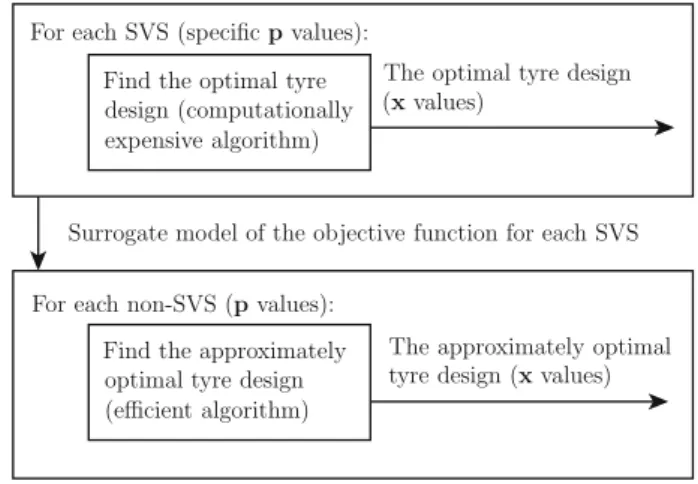
For each SVS (specificpvalues): Find the optimal tyre design (computationally expensive algorithm)

The optimal tyre design (xvalues)

Surrogate model of the objective function for each SVS

For each non-SVS (pvalues): Find the approximately optimal tyre design (efficient algorithm)

The approximately optimal tyre design (xvalues)

Fig. 1 Illustration of the proposed algorithm for the truck tyre design problem. Both the operating envi-ronment specification and the vehicle configuration are represented by parameters,p, while the tyre design is represented by the decision variables,x. Optimal solutions to the design problem for the SVSs operating in the most common environments are found using a computationally expensive optimization method, after which approximately optimal solutions for other vehicle configurations/operating environment specifications are computed efficiently by the proposed methodology

1.2 Motivation

The present sales tool at Volvo GTT generates a large set of feasible tyres for each truck. The truck tyres selection process is then based on experience and customer input that can be further improved by means of scientific methodologies. Volvo GTT’s ultimate goal is to find an optimal design of the tyres for each vehicle configuration and operating environment specification, with respect to minimizing the energy losses caused by the tyres. In the present phase of our research project (Lindroth2015), the tyres are described by continuous design variables (tyre diameter, tyre width, and inflation pressure). Our future research will introduce discrete design variables representing the tyres available in a tyre database, i.e., solving the so-calledtyres selection problem.

The number of vehicle configurations that can be manufactured by Volvo is huge; the same holds for the variety of environments in which the vehicles are operated. Solving the tyre design problem is very time consuming and computationally expensive, since (1) for each operating environment a sufficiently detailed vehicle model—including finite element models of the tyres—has to be run, and (2) the vehicle specification and operating environment models have to be adapted to each customer. One can afford to search for an optimal tyre design only for a small subset of all combinations of vehicle configuration and environment specification, i.e., only for the SVSs operating in the most common environments. For the non-SVS vehicles, the tyre design problem must be solved in real time during the sales process. Hence, for the non-SVS vehicles an algorithm that quickly finds an approximately optimal tyre design is needed in place of the computationally intractable search for an optimal tyre design.

Most of the energy losses caused by the tyres stem from the rolling resistance (Walter and Conant1974). The main ingredient in our model of the tyre design problem is therefore the rolling resistance coefficient (RRC). A finite element model of a truck tyre (Ali et al.2013) was used; this model allows for an investigation of the influence on the RRC of the tyre design variables and of the parameters describing the vehicle and the operating environment.

Each evaluation of the model takes, however, around four hours of computation time. The function that describes the RRC is influenced more significantly by the values of the tyre design variables than with those of the parameters describing the vehicle and its typical operating environment; see Ali et al. (2013). This property of the RRC will be used for assembling designs for non-SVSs vehicles, based on their corresponding positions in the parameter space; see Fig.1.

1.3 Outline

The remainder of this article is organized as follows. Algorithms utilized for the minimization of simulation-based functions, with a main focus on RSMs based on RBF interpolation, are reviewed in Sect.2. The algorithm suggested for solving many instances of a simulation-based optimization problem with a partitioned decision space is presented in Sect.3. The methodology used to assess the performance of the algorithm, the set of test problems selected, and the results from the test are presented in Sect.4. Finally, Sect.5provides conclusions as well as topics for future research.

2 Minimizing simulation-based functions

We aim to solve a set of simulation-based optimization problems possessing computationally expensive black-box objective functions. Letx∈RMdenote the vector of decision variables, p∈RD−M with 1≤ M ≤ D1denotes the vector of parameters, and f :RD →Ris the computationally expensive objective function, which is evaluated through simulations. The vectorslx < ux ∈RM andlp <up ∈RD−M define lower and upper bounds on the vari-ables and parameters, respectively. The simulation-based optimization problem considered is then to

minimize x∈[lx,ux]

f(x,p), (1)

for possibly many values ofp∈ [lp,up]. The requirement thatx∈ [lx,ux]is referred to as box constraints.

In this section we examine methods for the optimization of the problem (1) overx. We assume that the function modelling the RRC [represented in (1) by the functionf] is con-tinuous, which motivates the use ofcontinuous surrogate models; cf. Sect.2.1. Since the simulations of the objective function are computationally expensive the number of function evaluations should be kept at a minimum. Within the engineering community, RSMs are popular for solving such simulation-based optimization problems (Jones2001).

2.1 Response surface methods (RSMs)

Response surfaces provide fast computations of surrogate functions in place of time-consuming simulations. By running the simulation for a set of sample points and fitting an analytical function to the resulting function values, a computationally cheap surrogate model of the function is obtained and can be used for optimization purposes. The initial set of sample points may, e.g., be determined by adesign of experimentstechnique (see the review in Simpson et al.2001). Then additional points are sampled and evaluated (through a simulation) in order to refine the approximation of the true function, until a stopping criterion is met (e.g., a maximum allowed number of simulations is attained, or the function value 1_p∈ZD−M_{can also be considered with the same methodology.}

being below a given target). The strategies for selecting the sample points differ among spe-cific algorithms. An efficient strategy should balance local and global searches (Jakobsson et al.2010), such that the information from the surrogate model is utilized and no interesting part of the variable domain is left unexplored. Algorithm1summarizes a general RSM.

Algorithm 1General response surface method (RSM) for the optimization problem (1) for p= ¯p

0: Create an initial set of sample pointsx¯n ∈ [lx,ux],n ∈ {1, . . . ,N}, and evaluate f(x,p¯)for allx ∈

{¯x1, . . . ,x¯N}.

1: Construct a surrogate model off(·,p¯)from the points evaluated, i.e.,(x¯n,f(x¯n,p¯)),n∈ {1, . . . ,N}. 2: Select and evaluate a new sample pointx¯N+1to refine the surrogate model.

3: If a stopping criterion is met, exit. Otherwise, letN:=N+1 and go to step 1.

Assuming that the simulations of the true function do not exhibit a high degree of compu-tational noise, the shape of the function is usually better captured by an interpolating response surface—passing through all sample points—than by a non-interpolating surface—found by, e.g., minimizing the sum of squared errors at the sample points—which may be quite distant from the function values at the sample points (Wendland2005, Section 1.5). The interpolat-ing surface is typically constructed as a linear combination ofpolynomialandbasis function terms. Our development is based on an RSM which uses an RBF interpolation, originally presented in Powell (1999). Our algorithm can, however, utilize any kind of response surface (here also referred to as surrogate model).

2.2 Radial basis function interpolation

The surrogate model based on an RBF interpolation is formally defined below.

Definition 1 (radial basis function, RBF) Letting·denote the Euclidean norm, a function g : RM → R is called aradial basis function if there exists a univariate functionφ : [0,∞)→Rsuch that

g(x)=φ(x), x∈RM.

Assume that the objective function f(·,p¯)of (1) is simulated atNdistinct sample points ¯

xn ∈ [lx,ux] ⊂RM,n=1, . . . ,N. Denote the vector of function values at these points by ¯

f :=f(x¯1,p¯), . . . ,f(x¯N,p¯)T ∈RN, and the vector of variables byx=(x1, . . . ,xM)T.

The RBF interpolationSα:RM →Rof f(·,p¯)is then defined (Wendland2005, Section 6.3) as S_α(x):= N n=1 αnφ(x− ¯xn)+αN+1+ M m=1 αN+1+mxm, (2)

whereφ denotes a given RBF, e.g., a linear, multi-quadratic, or cubic function, andαn,

n=1, . . . ,N +1+M, are the interpolation coefficients. The interpolation problem is that to find a vectorα∈RN+1+Msuch that

A P PT 0 α= _¯ f 0 , (3) whereAi j :=φ(¯xi− ¯xj),i,j=1, . . . ,N, andPi·:=(1, (x¯i)T),i=1, . . . ,N.

The assignment (2) defines the unique RBF interpolationS_α of the unknown function f(·,p¯)at the sample pointsx¯n,n=1, . . . ,N, where the vectorαis uniquely determined by

the system (3) of linear equations (Wendland2005, Section 6.3). The RBF interpolation often yields good global representations of computationally expensive simulation-based functions, as judged by the errors estimated in Buhmann (2003, Chapter 5), and is therefore frequently used within RSMs.

3 Solving many instances of a simulation-based optimization problem

with a partitioned decision space

We assume that the objective functionf of (1) over the box defined by the constraints on the variablesxand the parameterspis influenced significantly more by the variables than by the parameters, over the respective boxes. This assumption is characterized by the relation between the approximation errors, whenf is approximated by 1st order Taylor expansions with respect toxandp, respectively, according to Assumption1.2

Assumption 1 For the partition(x,p), define Tx:=sup x,x¯,p f(x,p)−f(x¯,p)−Dxf(x¯,p)T(x− ¯x) x− ¯x x,x¯∈[lx,ux],p∈[lp,up] and Tp:=sup x,p,p¯ f(x,p)−f(x,p¯)−Dpf(x,p¯)T(p− ¯p) p− ¯p x∈[lx,ux],p,p¯∈[lp,up] . Then, the relationTx Tpis assumed to hold.

To identify the variables to be treated as parameters (i.e., the second argument, denotedp) one can perform a simple parameter study or a sensitivity analysis; alternatively the parameters may be identified from literature on existing models of the specific computationally expensive function studied.

Each instance of the problem (1) is determined through a selection of values for the parameter vectorp. The optimization problem (1) will be solved to near-optimality forQ selected parameter values, denotedp¯q,q =1, . . . ,Q. The other parameter settings, which are not known in advance and for which the problem (1) is to be (approximately) solved in a computationally efficient way, are denotedp¯r,r = Q+1, . . . ,Q+R(the value ofR may be unknown). It is desirable that the degree of nonlinearity off with respect topis low since it can be shown that iff is linear inp, then its RBF interpolationS_αwill be linear inp as well. Whenf is almost linear with respect topthe precision of the surrogate models for the parameter settingsp¯r,r = Q+1, . . . ,Q+R, will be as high as the precision of the surrogate models forp¯q,q=1, . . . ,Q.

Section3.1introduces two standard solution methods for solving the set of optimization problems (1). These methods will be used as a benchmark for the proposed methodology described in Sect.3.2.

3.1 Standard solution methods

Algorithm2is a standard solution method for the set of optimization problems (1) correspond-ing to the parameter settcorrespond-ingsp¯1, . . . ,p¯Q+R. It applies an RSM based on an RBF interpolation 2_{In Assumption1, the entitiesD}

xfandDpfdenote numerical partial derivatives offwrt.xandprespectively,

(see, e.g., Jakobsson et al.2010) of the functionf that is valid for allp∈ [lp,up]and will be used as a benchmark for the proposed methodology.

Algorithm 2An optimization algorithm based on response surfaces for a set of simulation-based optimization problem instances

0: Create a set ofNQsample points(x¯n,p¯n), such that(x¯n,p¯n)∈ [lx,ux] × [lp,up],n=1, . . . ,N Q,and

evaluate (simulate)f on this set.

1: Construct a surrogate modelSαoff using the points evaluated, according to (2) and (3) withxreplaced by(x,p).

2: Forq=1, . . . ,Q+R, find

xq_opt∈ argmin

x∈[lx,ux]

S_α(x,p¯q). ₍₄₎

The sample points created in Step 0 of Algorithm2are randomly generated in order to be uniformly distributed over the feasible set. We prioritize global search (exploration) when selecting the sample points in order to obtain a good global representation of the objective function, but any sophisticated rule for selecting sample points can be employed; see, e.g., Gutmann (2001, Algorithm 3). The total number of evaluations off is upper bounded by the valueNQ. For each instanceq ∈ {1, . . . ,Q+R}of (1), the desired optimal solutionxq_optis obtained by applying Algorithm2.

Another natural approach is to first choose the values ofp¯1, . . . ,p¯Q+R, and then—for each parameters settingp¯q—call a standard algorithm for solving simulation-based optimization problems returning the optimal values ofx_optq ,q=1, . . . ,Q+R. Such an approach allows the use of more sophisticated simulation-based optimization methods for both continuous and integer variablesx; see Jones et al. (1998), Björkman and Holmström (2000) and Hong et al. (2015). We will use the easy to use software application for simulation-based optimization, NOMAD (Abramson et al.2017), as the standard algorithm to find the optimal values of xq_opt. NOMAD is based on the Mesh Adaptive Direct Search (MADS) algorithm (Audet and Dennis2006). A potential drawback of this approach is that onlyN Q/(Q+R)sample points can be used to find eachxq_opt,q=1, . . . ,Q+R, and that the value ofQ+Rhas to be known in advance. This approach also cannot be used to solve the tyre design problem, in which all the simulations of the objective function are required to be done in a preprocessing phase. 3.2 The proposed methodology

We propose Algorithm3below to solve a set of optimization problems (1). It includes a preprocessing phase, in which, forpq,q = 1, . . . ,Q, selected settings of the parameter vector, a nearly-optimal solutionxq_optto (1) is computed provided that enough simulations off can be performed. Then, for any other values ofp∈ [lp,up], an approximately optimal solutionxr_approxis efficiently computed without any additional simulations of the expensive functionf; see Fig.2. The desired solutions to the optimization problem (1) for all parameter settings are computed using the response surface method (Algorithm1), i.e., a surrogate function is minimized instead of the true objective functionf.

The sample points in Step 1a of Algorithm3are randomly generated to be uniformly distributed over the feasible set. We prioritize global search (exploration) when selecting the sample points to obtain a good global representation of the objective function, but any sophisticated rule for selecting sample points can be employed; see, e.g., Gutmann (2001,

Fig. 2 Flowchart illustrating Algorithm3for the optimization of a set of simulation-based optimization problem instances

Algorithm 3An efficient optimization algorithm based on weighted response surfaces for a set of simulation-based optimization problem instances

1: For eachq=1, . . . ,Q:

a: Select a distinct parameter settingp¯q ∈ [lp,up]. Create a set ofN sample pointsx¯n, such that

¯

xn∈ [lx,ux],n=1, . . . ,N, and simulatef(x¯n,p¯q),n=1, . . . ,N.

b: Construct a surrogate modelS_αq(·,p¯q)according to (2) and (3) and find

x_optq ∈ argmin

x∈[lx,ux]

S_αq(x,p¯q). ₍₅₎

2: For eachr=Q+1, . . . ,Q+R:

a: Construct a surrogate modelS_αr(·,p¯r)according to (2), letting the vectorαr ∈RN+1+Dof inter-polation coefficients be a convex combination (e.g., assigned as in (8), below) of the initial vectors of coefficients,αq, according to αr_:= Q q=1 wr qαq, Q q=1 wr q=1, wr q≥0,q=1, . . . ,Q. (6)

b: Compute an approximate optimal solution to (1), forp= ¯pr:

xrapprox∈ argmin x∈[lx,ux]

S_αr(x,p¯r). ₍₇₎

Algorithm 3). The same set of sample pointsx¯n,n=1, . . . ,N, is used for all surrogate models in Step 1a, since then the surrogate modelS_αr(·,p¯r)can be found directly by weighting the

interpolation coefficients.3 _{The number of evaluations of the functionf is limited toNQ,} i.e., the same number as for Algorithm2. The optimization problems (4) and (5) are solved 3_{When using a different set of sample points for each parameter setting, the function values must instead be}

weighted and the interpolation coefficients have to be found by solving the system (3). The approach using different sets of sample points for different parameter settings results in the sample points being more spread over the search space. Experiments indicate that more accurate approximationsxrapprox,r=Q+1, . . . ,Q+R,

because we are interested in near-optimal solutions to (1) for the selected parameter settings (the optimal tyre designs for the SVSs can then be used to point out the tyre designs to be improved with respect to the RRC, e.g., by adjusting their groove patterns).

The surrogate modelsSαq(·,p¯q):RM →Rconstructed in Step 1b of Algorithm3are

defined onRM, since the second argumentp¯q of the functionf is fixed over theN sample points. The optimal solutionsxq_opt are not used further in the algorithm, but given to the practitioner. For the tyre design problem the optimal solutionsxq_optare used to identify the strategic tyre designs to be further improved wrt. fuel efficiency.

Each of the surrogate modelsS_αr(·,p¯r) :RM → R, r = Q+1, . . . ,Q+R, is

con-structed (in Step 2a of Algorithm 3) as a convex combination4 of the surrogate models S_αq(·,p¯q),q=1, . . . ,Q. For eachr∈ {Q+1, . . . ,Q+R}, the values of the convex

com-bination coefficients—here also referred to asweights—wr qofαq, in the surrogate model

S_αr(·,p¯r), are defined according to (6), and as a function of the values ofp¯randp¯q ∈ [l_p,u_p],

q =1, . . . ,Q. Provided thatp¯r _{= ¯p}q_{,q =1, . . . ,Q, the weights may, e.g., be defined as}

inversely proportional to the Euclidean distance betweenp¯randp¯q:

wr q:= ⎛ ⎝_¯pq − ¯pr Q t=1 1 ¯pt_{− ¯p}r ⎞ ⎠ −1 , q=1, . . . ,Q. (8)

In our test cases—for implementation simplicity—only the two parameter vectorsp¯q1 _and

¯

pq2 _{being closest}5 _{to the parameter vectorp}¯r, _r = _Q+₁, . . . ,_Q+_{R, are given nonzero} weights,wr q1 andwr q2, respectively. Several alternative principles for defining the weights

wr qmay be employed. For example, they can be defined by more than two parameter vectors,

higher weights can be assigned to surrogate models for values ofpfor which the surrogates are expected to be more accurate, or a priori known properties of the functionf (e.g.,f being quadratic with respect top) can be utilized.

No additional simulations of the objective functionf are needed to compute the approxi-mately optimal solutionxr_approxof (7) in Step 2b of Algorithm3. This constitutes a significant computational saving [as compared to solving (7) for eachp¯r _{individually, which requires}

a new set of sample points to construct the surrogate modelSαr(·,p¯r)] and allows for the

computation of approximately optimal solutions in real time.

The main advantage of Algorithm 3 as compared to Algorithm2 is that the lower-dimensional box[lx,ux] ⊂RMis sampled for each of the selected settings ofp∈ [lp,up] ⊂

RD−M_{, instead of sampling the whole set[l}

x,ux] × [lp,up] ⊂RD.

General RBF interpolating methods yield more and more accurate interpolations as new sample points are added. According to Buhmann (2003, Theorem 5.5), for locally Lipschitz continuous functionsf, as the set of sample points grows dense in the domain, the surrogate function S_α converges to the true functionf on this domain, which implies that the error estimate of the interpolation tends to zero. When considering a simulation-based functionf we cannot presume that it is locally Lipschitz continuous and the performance of Algorithm3 has to be assessed through computational experiments.

4_{The use of a convex combination is motivated by (i) the assumption that the objective functionfis influenced}

significantly more by the variables than by the parameters, and (ii) the assumption that the parameter values ¯

pq,q=1, . . . ,Q, are spread over the box[lp,up]. Iffis linear inp, then the RBF interpolationSαris equal to the convex combination ofS_αq,q=1, . . . ,Q.

5_q

4 Computational experiments

The purpose of the computational experiments is to compare the performance of Algorithms2 and3and NOMAD applied to a set of simulation-based optimization problems. The test problems, whose properties resemble those of the tyre design problem that we wish to solve, were collected from Gould et al. (2003) and Montaz Ali et al. (2005) and are often used for testing optimization algorithms aiming at convergence to a global optimum.

The methodology used for assessing the performance of the algorithms tested, as well as the performance measures used, are introduced in Sect.4.1. The test problems are described in Sect.4.2. Section4.3discusses the implementation details, while Sect.4.4summarizes the test results. Section4.5describes how the tyre design problem can be solved using the algorithm developed.

4.1 Performance measures and methodology

This section presents thesuccess ratio, designated to compare the effectiveness and the trustworthiness of algorithms, as well as theperformance profileanddata profile, designated for more complex comparisons of algorithms.

Success ratio

LettingAbe the set of tested algorithms andPbe the set of test problems, the success ratio sap∈ [0,1]equals the number of times that algorithma∈Asuccessfully approximates an

optimum to the problemp∈Pdivided by the number of times that the algorithm is applied to solve the problemp(Törn and Žilinskas1989, Ch. 1).

Consider the instance r of problem p of the form (1) defined by p = ¯pr, and let Xr

opt ⊂ [lx,ux] ⊂RM denote its optimal set. An algorithma ∈Ais said to successfully approximate its optimal solution if the resulting point is feasible and lies in a sufficiently small neighbourhood of the set of optimal solutions, i.e., ifxr_approxbelongs to the set

N_εp(Xr_opt):= x∈ [lx,ux]miny∈Xr optx−y ≤εp , (9) whereεp>0 is a tolerance parameter. For each problempthe value ofεpis determined by

the size and dimension of the box[lx,ux]and is reported in “Appendix”.

For all the algorithms tested, the same number of points are sampled. In Algorithm2, all the sample points are used to map a subspace ofRD, while in Algorithm3the number of sample points is divided, so that half of them are used to sample a subspace ofRM(where M<D) for each of the two selected parameter vectors, i.e.,Q=2. When NOMAD is used the number of sample points is divided as well: two thirds of them are used to sample the subspacesRMfor each of the two selected parameter vectors, and one third is used to solve the problem forQ+1, i.e., to findxapproxQ+1 .

Performance and data profile

Theperformance profileintroduced in Dolan and Moré (2002) has been utilized for com-paring the performance of Algorithms2and3on the whole set of test problems considered simultaneously. The performance profile for an algorithm is defined as the (cumulative) dis-tribution function for a performance metric, here represented by the number of sample points. Assuming a setAof algorithms applied to a setPof problems, for eachp∈Panda∈A,

tpais defined as the number of sample points used to successfully approximate (in the

vari-able space) an optimum of the problempby algorithma. Theperformance ratio, defined as tpa(minb∈A{tpb})−1, p∈P, a∈A,relates the performance of algorithmaas applied to

the problempto the best performance of any of the algorithms in the setA. If algorithmais not able to successfully approximate an optimum to the problemp(i.e., iftpa>T for some

large valueT >0), then the performance ratio is set to a constantcap>maxb∈A\{a}{tpb}. An

overall assessment of the performance of algorithmais obtained by defining the probability that the performance ratio is within a factorτ ≥1 of the best attained ratio for any of the algorithms, i.e., ρa(τ):= 1 |P| ⎧ ⎨ ⎩p∈P: tpa min b∈A{tpb} ≤τ ⎫ ⎬ ⎭ ,

where|·|denotes cardinality. The functionρa: [1,∞)→ [0,1]is the cumulative distribution

function of the performance ratio.

A plot of the performance profile for the setAof tested algorithms reveals the major performance characteristics of the algorithm but does not provide sufficient information to a user with a computationally expensive optimization problem, who is often more interested in the performance of solvers as functions of the number of function evaluations. We thus use thedata profileof an algorithma∈Aintroduced in Moré and Wild (2009), defined as the percentage of the problems that are solved at the cost ofτ >0 withnpbeing the number

of variables of problemp∈P, i.e., da(τ):= 1 |P| p∈P: tpa np+1 ≤τ .

The unit of cost isnp+1 function evaluations which can be easily translated into function

evaluations. This unit can be interpreted as the percentage of problems that can be solved with the equivalent of simplex gradient estimates,np+1 referring to the number of evaluations

needed to compute a one-sided finite-difference estimate of the gradient.

Performance profiles compare the different algorithms, while data profiles provide, for each given algorithm (independent of the other algorithms), the proportion of the problems that are solved within a certain number of function simulations normalized by the corre-sponding number of variables by a given algorithm. We will present both performance and data profiles for the test problems considered.

Assessment methodology

The overall methodology used to assess and compare the performance of Algorithms2and 3is described next. The sample pointsx¯n,n=1, . . . ,N Q, were randomly generated to be uniformly distributed over the feasible sets. Also the latin hypercube design of experiments (Sóbester et al.2014) was tested to generate the sample points, but since the resulting improve-ments of the success of approximation of an optimal solution—as compared with randomly generated sample points—was negligible we chose to use sample points with randomly gen-erated coordinates over their respective feasible intervals (using Matlab’s pseudo-random number generator). Considering the various measures for comparing algorithms discussed in this section, the following experimental procedure, inspired by Montaz Ali et al. (2005), was established.

1. Assemble a setPof test problems from the literature. For each of the problems chosen, record the variables and objective values at an optimal solution (or at the best known solution).

2. Choose the numberNQof sample points (i.e.,x¯n) to create. For each problem: perform 30 runs each of Algorithms2and3.

3. For each problempand each algorithma, record the success ratiosap.

4. Increase the numberNQof sample points. Repeat from step 2 until either Algorithm2 or Algorithm3successfully approximates an optimum for each problemp.6

5. Generate the performance and data profiles.

The success ratio is used when repeated runs of an optimization algorithm may give different results, which is the case for Algorithms2and3, which use randomly generated sample points. When using NOMAD the sample points are deterministically generated, creating a mesh. Hence, it is enough to apply NOMAD once per problem and therefore its success ratio will not be reported.

4.2 Test problems

The experimental procedure described in Sect.4.1 has been applied to 22 selected box-constrained optimization problems with continuous variables; these are denoted p ∈ {1, . . . ,22}below. These problems (except for p∈ {6,7,12,16,20,21}) form a subset of a test-bed for global optimization solvers originally proposed in Montaz Ali et al. (2005), and include both artificial and real problems; see Table 1and “Appendix”. To make the tests demonstrative, problems differing in dimension, computational difficulty, and number of known local optima are selected. Most of them are considered as fairly easy in terms of global optimization; when viewed as simulation-based optimization problems—in which normally no analytical information can be exploited—they are, however, challenging.

The proposed algorithm is developed for optimization problems in which the influence of some of the variables on the value of the objective function is less significant than that of the rest of the variables and one wants to solve many instances of the problem. The less influencing variables are then treated as parameters, denoted by the vectorp. From the 50 test problems proposed in Montaz Ali et al. (2005) in fifteen problems (1, 3–5, 8–11, 13–15, 17– 19, and 22) the less influencing variables are identified based on the definition of significant influence in Assumption1and will be used to asses the performance of Algorithm3. Problem 2 is included in order to demonstrate the performance of the algorithm when applied to a problem for which the objective function is influenced equally by all its variables. The Problems 6, 7, 12, 16, 20, and 21 (taken from Schwefel1981; Bersini et al.1996; Dixon and Price1999; Gould et al.2003; Rahnamyan et al.2007, and gathered in Jamil and Yang2013) are considered in order to test the algorithms for a larger number of variables, for which Algorithm3is intended.

The tyre design problem in the current implementation contains four variables and 55 parameters; hence, its dimensions D andM are similar to Problem 7. The results from Algorithm3applied to this problem will be commented on below.

6_{See the definition ofN}

εp(Xropt)in (9), where the values of the tolerance parameterεp>0 differs between

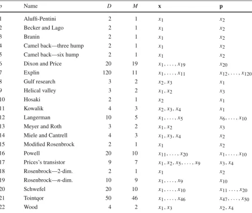
Table 1 Data for the test problems: problem number (p), problem name, problem dimension (x ∈RM,

p∈RD−M), and partition into variablesxand parametersp

p Name D M x p

1 Aluffi-Pentini 2 1 x1 x2

2 Becker and Lago 2 1 x1 x2

3 Branin 2 1 x1 x2

4 Camel back—three hump 2 1 x1 x2

5 Camel back—six hump 2 1 x1 x2

6 Dixon and Price 20 19 x1, . . . ,x19 x20

7 Explin 120 11 x1, . . . ,x11 x12, . . . ,x120 8 Gulf research 3 2 x2,x3 x1 9 Helical valley 3 2 x1,x2 x3 10 Hosaki 2 1 x2 x1 11 Kowalik 4 3 x2,x3,x4 x1 12 Langerman 10 5 x1, . . . ,x5 x6, . . . ,x10

13 Meyer and Roth 3 2 x1,x2 x3

14 Miele and Cantrell 4 3 x1,x3,x4 x2

15 Modified Rosenbrock 2 1 x1 x2 16 Powell 20 10 x11, . . . ,x20 x1, . . . ,x10 17 Prices’s transistor 9 7 x1,x2,x5, . . . ,x9 x3,x4 18 Rosenbrock—2-dim. 2 1 x1 x2 19 Rosenbrock—n-dim. 10 9 x1, . . . ,x9 x10 20 Schwefel 20 10 x1, . . . ,x10 x11. . . ,x20 21 Tointqor 50 46 x1, . . . ,x46 x47, . . . ,x50 22 Wood 4 2 x1,x3 x2,x4

See “Appendix” for detailed descriptions of the problems and the corresponding references

4.3 Implementation

We implemented the efficient optimization algorithm for a set of simulation-based problem instances (Algorithm3) and the standard optimization algorithm based on an RBF interpola-tion (Algorithm2) in MATLAB R2010b (The MathWorks, Inc.2012). All experiments were carried out on a desktop computer equipped with Intel Pentium Dual-Core 2.80 GHz and 4 GB RAM, running Red Hat Enterprise Linux 5.6. To optimize the nonlinear interpolation func-tionsS_αgenerated during the various steps of the algorithms, subject to box constraints, the external solver glbFast from the TOMLAB/CGO v8.0 toolbox for global optimization (Holm-ström and Göran2002) was used; it solves box-constrained global optimization problems using only function values, and is based on the DIRECT algorithm from Jones et al. (1993). In our implementation of Algorithms2and3the simple linear RBFg:RD→R₋, defined byg(x) = φ(x) := −x, was employed in order to construct the RBF interpolations (2). We have allowed NOMAD to use Latin-Hypercube Search and Variable Neighbourhood Search when it got stuck in a local optimum, in order to improve its performance and use the same number of sample points as the other algorithms tested.

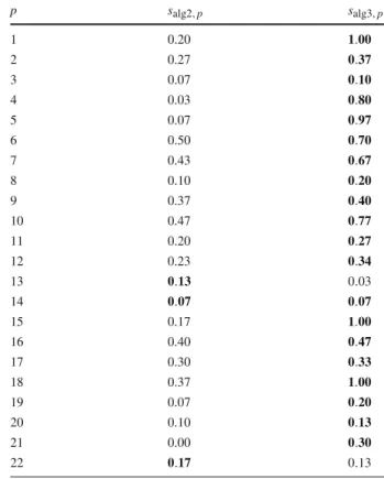
Table 2 Success ratios for Algorithm2(denoted alg2) and Algorithm3(denoted alg3)

p s_alg2,p salg3,p 1 0.20 1.00 2 0.27 0.37 3 0.07 0.10 4 0.03 0.80 5 0.07 0.97 6 0.50 0.70 7 0.43 0.67 8 0.10 0.20 9 0.37 0.40 10 0.47 0.77 11 0.20 0.27 12 0.23 0.34 13 0.13 0.03 14 0.07 0.07 15 0.17 1.00 16 0.40 0.47 17 0.30 0.33 18 0.37 1.00 19 0.07 0.20 20 0.10 0.13 21 0.00 0.30 22 0.17 0.13 4.4 Results

A general optimization algorithm converges to the global optimum for every continuous objective functionf if and only if the set of sample points grows dense over the feasible domain; see Gutmann (2001, Theorem 4). Nevertheless, the determination of an acceptable result after a reasonably small number of function evaluations is often its most desirable feature. Therefore, the quality of our optimization algorithm for simulation-based functions is demonstrated through its practical use for solving representative test problems utilizing relatively few function evaluations.

The success ratios for Algorithms2and3—possessing values in the interval[0,1]—are listed in Table2. Each bold entry indicates the algorithm that performs the best when applied to the respective test problem.

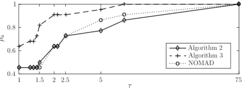
In Figs.3and4, the performance profiles (Dolan and Moré2002) and data profiles (Moré and Wild2009) of Algorithms2and3and NOMAD over the 22 test problems considered are illustrated. Algorithm3, which is proposed in this paper, clearly outperforms both NOMAD and Algorithm2(being a version of Algorithm1, adjusted in order to suit the specific problem considered, but which does not utilize the partition(x,p)) for the problems tested. In the worst case Algorithm3needed approximately twice as many sample points as the other algorithms. Figures5and6, respectively, illustrate the performance and data profiles of Algorithms2 and3and NOMAD over the larger test problems considered, i.e., (6, 7, 12, 16, 17, and 19–21). Algorithm3, developed for solving a set of simulation-based optimization problem

ρa τ Algorithm 2 Algorithm 3 NOMAD 1 1 5 0.8 0.6 0.4 2.5 75 2 5 . 1

Fig. 3 Performance profiles of Algorithms 2 and 3 and NOMAD for the 22 problems tested. The graphs represent the portion ρa of the problems that are successfully approximated (see Sect. 4.1;

the value of the tolerance parameter εp varies among the test problems) within a factor τ ∈

{1,1.25,1.33,1.43,1.5,2,2.15,2.5,5,8,75}times the number of sample points used by the algorithm that successfully approximates an optimal solution using the smallest number of sample points. The scale used for the horizontal axis is logarithmic

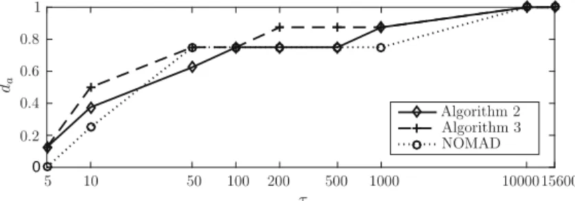
da τ Algorithm 2 Algorithm 3 NOMAD 1000 100 200 500 1000015600 0 5 1 0 0.2 5 10 0.8 0.6 0.4

Fig. 4 Data profiles of Algorithms2and3and NOMAD for the 22 problems tested. The graphs represent the portiondaof the problems that are successfully approximated (see Sect.4.1; the value of the tolerance parameter

εp varies among the test problems) withinτ(np+1) ∈ {5,10,50,100,200,500,1000,10,000,15,600}

sample points used. The scale used for the horizontal axis is logarithmic

instances in a computationally efficient way, turned out to be particularly suitable for the larger problems considered.

We next discuss the cases when the algorithm developed performed worse than the standard RSM and NOMAD:

– Both Algorithms2and3terminate at inaccurate approximations of the global optimum of Problem 13; this is probably because the objective function decreases steeply towards the global minimum in a small area, which is difficult to locate with only a small number of randomly generated sample points. Hence, another (more sophisticated) rule for selecting sample points should be employed. NOMAD outperforms both Algorithms2and3on Problem 13 because new sample points are generated based on the function values at the old sample points.

– Both Algorithms2and3find inaccurate estimations of the optimal objective value of Problem 17, because the objective function is oscillating around the global optimum. A more suitable surrogate model should be chosen for Problem 17 in order to obtain more accurate estimations of the optimal objective value. NOMAD is not based on any surrogate model so the estimation of the optimal objective value of Problem 17 is more accurate but corresponds to a less accurate approximation of the global optimum.

ρa τ Algorithm 2 Algorithm 3 NOMAD 1 1 0.2 5 0.8 0.6 0.4 2.5 75 2 5 . 1

Fig. 5 Performance profiles of Algorithms2and3and NOMAD for the larger problems (6, 7, 12, 16, 17, and 19–21) tested. The graphs represent the portionρaof the problems that are successfully approximated

within a factorτ∈ {1,1.25,1.33,1.43,1.5,2,2.15,2.5,5,8,75}times the number of sample points used by the algorithm that successfully approximates an optimal solution using the smallest number of sample points. The scale used for the horizontal axis is logarithmic

da τ Algorithm 2 Algorithm 3 NOMAD 10 50 100 200 500 1000 10000 15600 1 5 0.8 0.4 0.2 0.6

Fig. 6 Data profiles of Algorithms2and3and NOMAD for larger problems (6, 7, 12, 16, 17, and 19– 21) tested. The graphs represent the portionda of the problems that are successfully approximated (see

Sect.4.1; the value of the tolerance parameterεp varies among the test problems) withinτ(np+1) ∈

{5,10,50,100,200,500,1000,10,000,15,600}sample points used. The scale used for the horizontal axis is logarithmic

– Even though it is not possible to decide which variable should be treated as a parameter in Problem 2 (the objective function is quadratically influence by each of the variables), Algorithm3yields more accurate results than Algorithm2.

The performance of NOMAD increases with an increasing number of sample points used. When solving a large number of instances of (1) using only a limited number of sample points, NOMAD will lead to inaccurate approximations of the global optima; see Figs.3 and4.

We compared the approximate solutions to the test problems resulting from partitions of the decision variables (into the variablesxand the parametersp), being either randomly selected or based on a priori information about the objective function. Algorithm3produces more accurate approximations of the optimal solutions for the partitions based on a priori information than for the randomly selected partitions. For an equal number of sample points, the approximate solutions computed by the computationally efficient Algorithm3are in most cases still more accurate than the ones resulting from the application of Algorithm2.

Problem 7, for which it is obvious from the explicit expression of the objective function how to choose the variablesx∈RM and parametersp∈RD−M, was selected in order to investigate how the relative sizes of the sets of variables/parameters influence the performance of Algorithm3. The accuracy of the approximately optimal solution obtained does not appear

to be influenced by the ratio M_D for the same number of sample points, whereas the lowest value of the objective function is reduced when this ratio is decreased. From this we conclude that as many variables as possible not significantly influencing the objective function should be treated as parameters in Algorithm3.

4.5 Application to the tyre design problem

Our aim is to apply Algorithm3to solve the tyre design problem in the combinatorial setting of vehicles and operating environments. The surrogate models of the objective function and the corresponding optimal tyre designs—for the strategic configurations of vehicles operating in the most common environments—are found in a pre-processing phase involving many computationally expensive simulations of the objective function (representing the energy losses caused by the tyres). An approximately optimal tyre design can then be found in a computationally efficient way (and which then can be implemented in the sales tool at Volvo) for any customer specifying the vehicle and its intended use, by using a weighted surrogate model of the objective function, as described in this article. The tyre design variables are so far considered to be continuous. We are currently developing the algorithm to incorporate also discrete requirements on the variable values. The algorithm developed can, however, be directly used for both continuous and discrete requirements on the parametersp; the individual vehicles in the tyre design problem then correspond to discrete values of the parameters.

A test instance of the tyre design problem is presented below. A Volvo rigid truck with four wheels with the two rear wheels driven is considered. The tyres are the same within each axle but can differ between the front and rear axles. Each tyre is determined by the values of three continuous variables (the tyre diameter, the tyre width, and the inflation pressure), resulting in a simulation-based optimization problem with the variable vectorx=(x1, . . . ,x6)T∈R6. Upper (ux=(ux1, . . . ,ux6)T) and lower (lx=(lx1, . . . ,lx6)T) bounds on the variables result in box constraints. Each evaluation of the objective function, which represents the energy losses caused by the tyres, requires a simulation of the vehicle over its operating environment; see Koláˇr (2015) for a description of the joint vehicle, tyres, and operating environment model used. The energy losses to be minimized are measured in MJ/km.

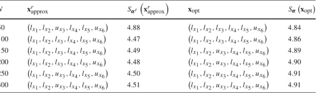
The parameterp∈Rwhich will be varied over the instances of the tyre design problem represents the topography of the operating environment. The other parameters, describing the truck, the operating environment, and the tyres, are kept fixed. The SVSs include the truck operating on a flat road and the same truck operating on a hilly road. Approximately optimal tyre designs (for both the front and rear axles) for the truck operating on a predominantly flat road are to be found by Algorithm3whenN sample points are used for each of the SVSs. The approximately optimal tyres designs are compared with the optimal tyre designs found when the tyre design problem for the truck operating on a predominantly flat road is solved directly using 2N sample points; see Table3.

The optimal solution to the tyre design problem for the truck operating on a predominantly flat road was found to be(lx1,lx2,ux3,lx4,lx5,ux6). Algorithm3successfully approximates the optimal designs while being computationally efficient when sufficiently many sample points can be used in the pre-processing phase for the strategic configurations operating in the most common environments, as can be seen in Table3. This fact does not cause any difficulties with the implementation of Algorithm3into the sales tool where the computational efficiency of finding the approximately optimal tyre designs for any customer is important. The optimal solution to the tyre design problem for the truck operating on a predominantly flat road was found to be a combination of the lower an upper bounds on the variable values. Therefore, additional constraints, such as the handling quality, the ride comfort, and the

Table 3 The approximately optimal tyre designsxrapproxfor the truck operating on a predominantly flat road,

and the corresponding energy lossesS_αr(xrapprox)(MJ/km), whenNsample points are used

N xrapprox Sαr xrapprox xopt Sαxopt 50 lx1,lx2,ux3,lx4,lx5,ux6 4.88 lx1,lx2,lx3,lx4,lx5,ux6 4.84 100 lx1,lx2,lx3,lx4,lx5,ux6 4.47 lx1,lx2,lx3,lx4,lx5,ux6 4.86 150 lx₁,lx₂,lx₃,lx₄,lx₅,ux₆ 4.49 lx₁,lx₂,ux₃,lx₄,lx₅,ux₆ 4.89 200 lx1,lx2,lx3,lx4,lx5,ux6 4.48 lx1,lx2,ux3,lx4,lx5,ux6 4.90 250 lx1,lx2,ux3,lx4,lx5,ux6 4.50 lx1,lx2,ux3,lx4,lx5,ux6 4.91 300 lx1,lx2,ux3,lx4,lx5,ux6 4.51 lx1,lx2,ux3,lx4,lx5,ux6 4.91 The optimal tyres designs found when the tyres design problem for the truck operating on a predominantly flat road is solved directly with 2Nsample points and the corresponding energy lossesSα(xopt)(MJ/km) are

listed for comparison

startability of the truck should be added to the optimization model of the tyre design problem and the simulation model of the objective function should be improved.

5 Conclusions and future research

A computationally efficient optimization algorithm—based on a radial basis function inter-polation adapted to a large set of simulation-based problem instances—has been developed, implemented, and tested. Our computational results demonstrate a performance of the algo-rithm which is superior to that of a standard response surface method (RSM) as well as NOMAD, when applied to a standard set of test problems. The algorithm is particularly suit-able when the differentiation of parameters and varisuit-ables can be distinctly resolved, and when aiming to solve efficiently the optimization problem at hand—at least approximately—for a large number of parameter settings. We consider problem settings possessing box constraints on the variables. The algorithm proposed can, however, be extended to solve optimization problems with more general (even simulation-based) constraints, then being relaxed and replaced by penalty terms in the objective function.

To compose surrogate models for any settings of the parameters, the algorithm utilizes aggregated surrogate functions of a set of selected parameter settings. Other models for the aggregation of the surrogate functions of the selected parameter settings should be inves-tigated. The algorithm may also be generalized to be applicable in the context of utilizing other kinds of surrogate models (e.g., Kriging interpolation or polynomial regression).

The algorithm developed enables the computationally efficient solution of the truck tyre design problem when described in the combinatorial domain of possible vehicle configura-tions and operating environment specificaconfigura-tions. Our future research includes incorporating discrete requirements on the variable values into the algorithm developed. This will enable the solution of a true tyres selection problem, in which the feasible tyres are taken from a tyre database, resulting in practically more useful solutions in place of the tyre designs resulting from the problem considered in this paper.

Acknowledgements The research leading to the results presented in this paper was financially supported by the Swedish Energy Agency (Project Number P34882-1), Chalmers University of Technology, and Volvo Group Trucks Technology. We acknowledge three anonymous referees for their valuable comments.

Open Access This article is distributed under the terms of the Creative Commons Attribution 4.0 Interna-tional License (http://creativecommons.org/licenses/by/4.0/), which permits unrestricted use, distribution, and reproduction in any medium, provided you give appropriate credit to the original author(s) and the source, provide a link to the Creative Commons license, and indicate if changes were made.

Appendix: Global optimization test problems

We present the 22 box-constrained test problems selected among problems that are frequently used for testing global optimization algorithms. Most of these problems are presented in Mon-taz Ali et al. (2005); however, the problems 6, 7, 12, 16, 20, and 21 are taken from Schwefel (1981), Bersini et al. (1996), Dixon and Price (1999), Gould et al. (2003) and Rahnamyan et al. (2007), respectively. The problems selected are suitable for testing the algorithm pre-sented because the significance of the influence on the function values differs between subsets of the variables. The only exception is Problem 2, which is selected in order to investigate whether the algorithm can be successful also when all of the variables influence the objective function to a similar extent. The tolerance parameterεp>0 is stated for each problemp.

1. Aluffi-Pentini problem(Aluffi-Pentini et al.1985): minimize

x∈R2 f(x):=0.25x

4

1−0.5x12+0.1x1+0.5x22,

subject toxi ∈ [−10,10],i =1,2. The problem has two local minima; one is global,

located at(−1.0465,0)T, with the optimal objective valuef∗≈ −0.3523. The tolerance parameter value isε1:=0.05.

2. Becker and Lago problem(Price1983): minimize

x∈R2 f(x):=(x1 −5)

2_+(x

2 −5)2,

subject toxi ∈ [−10,10],i = 1,2. The function has four global minima, located at (±5,±5)Twith f∗=0. The tolerance parameter value isε2:=0.025.

3. Branin problem(Dixon and Szegö1978): minimize

x∈R2 f(x):=a(x2−bx

2

1+cx1−d)2+g(1−h)cos(x1)+g,

wherea =1,b=5.1/(4π2),c=5/π,d =6,g=10,h =1/(8π), subject tox1 ∈ [−5,10]andx2 ∈ [0,15]. The global minima are located at(−π,12.275)T,(π,2.275)T, and(3π,2.475)T_{, with f}∗_{=5π/4. The tolerance parameter value isε}

3:=0.025. 4. Camel back—three-hump problem(Dixon and Szegö1978):

minimize x∈R2 f(x):=2x 2 1−1.05x14+ 1 6x 6 1+x1x2+x22,

subject toxi ∈ [−5,5],i =1,2. The problem has three local minima; one of them is

global, located at(0,0)Twith f∗=0. The tolerance parameter value isε4:=0.01. 5. Camel back—six hump problem(Dixon and Szegö1978):

minimize x∈R2 f(x):=4x 2 1−2.1x14+ 1 3x 6 1+x1x2−4x22+4x24,

subject to xi ∈ [−5,5],i = 1,2. The objective function is symmetric around the

origin and has three conjugate pairs of local minima, two of them are global, located at±(0.089842,−0.712656)T, with f∗≈ −1.0316. The tolerance parameter value is

6. Dixon and Price problem(Dixon and Price1999): minimize x∈R20 f(x):=(x1−1) 2₊ 20 i=2 i(2x_i2−xi−1)2,

subject toxi ∈ [0,10],i =1, . . . ,20. The global minimum is located atx_i∗=2−

2i−2

2i _,

i=1, . . . ,20, with f∗=0. The tolerance parameter value isε6:=0.05. 7. Explin problem(Gould et al.2003):

minimize x∈R120 f(x):= 10 i=1 exp(0.1xixi+1)+ 120 i=1 (−10i xi),

subject to xi ∈ [−10,10],i = 1, . . . ,120. The best known solution, which can be

found in Shcherbina et al. (2003), with f(x)= −723756.3, was obtained by the solver LINGO8 (Ding et al.2009). The tolerance parameter value isε7 :=10.

8. Gulf research problem(Moré et al.1981):

minimize x∈R3 f(x):= 99 i=1 exp −(ui−x2)x3 x1 −0.01i 2 ,

whereui=25+ [−50 ln(0.01i)]1/1.5, subject tox1 ∈ [0.1,100],x2 ∈ [0,25.6], and x3∈ [0,5]. The global minimum is located at(50,25,1.5)Twith f∗=0. The tolerance parameter value isε8:=0.25.

9. Helical valley problem(Wolfe1978): minimize x∈R3 f(x):=100 (x2−10θ(x))2+( (x₁2+x₂2)−1)2 +x₃2, where θ(x)= 1 2π tan−1xx21, ifx1≥0, 1 2π tan−1xx21 + 1 2, ifx1<0,

subject toxi ∈ [−10,10],i = 1,2,3. The objective function is a steep-sided valley

which follows a helical path. The global minimum is located at(1,0,0)Twith f∗=0. The tolerance parameter value isε9:=0.25.

10. Hosaki problem(Benke and Skinner1991): minimize

x∈R2 f(x):=(1−8x1+7x

2

1−7/3x13+1/4x14)x22exp(−x2),

subject tox1∈ [0,5],x2∈ [0,6]. There are two minima, of which the global minimum is located at(4,2)Twith f∗≈ −2.3458. The tolerance parameter value isε10:=0.01. 11. Kowalik problem(Jansson and Knüppel1995) (a least squares problem):

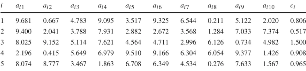
minimize x∈R4 f(x):= 11 i=1 ai− x1(1+x2bi) (1+x3bi+x4b_i2) 2 ,

subject toxi∈ [0,0.42],i∈1,2,3,4. The values ofaiandbiare given in Table4. The

global minimum is located at(0.192,0.190,0.123,0.135)Twith f∗≈3.0748×10−4. The tolerance parameter value isε11:=0.05.