Sparsity-Driven Statistical Inference for Inverse Problems

(1)

POUR L'OBTENTION DU GRADE DE DOCTEUR ÈS SCIENCES

acceptée sur proposition du jury: Prof. J.-Ph. Thiran, président du jury

Prof. M. Unser, directeur de thèse Prof. M. Figueiredo, rapporteur

Prof. R. Gribonval, rapporteur Prof. M. Vetterli, rapporteur

Sparsity-Driven Statistical Inference for Inverse Problems

THÈSE N

O

_{6545 (2015)}

ÉCOLE POLYTECHNIQUE FÉDÉRALE DE LAUSANNE

PRÉSENTÉE LE 27 MARS 2015

À LA FACULTÉ DES SCIENCES ET TECHNIQUES DE L'INGÉNIEUR LABORATOIRE D'IMAGERIE BIOMÉDICALE

PROGRAMME DOCTORAL EN GÉNIE ÉLECTRIQUE

Suisse 2015

PAR

(2)

Thèse présentée à la faculté des sciences et techniques de l’ingénieur pour l’obtention du grade de docteur ès sciences

Professor Jeau-Philippe Thiran, président

Professor Michael Unser, directeur de thèse

Professor Mario Figueiredo, rapporteur

Professor Rémi Gribonval, rapporteur

Professor Martin Vetterli, rapporteur

École polytechnique fédérale de Lausanne—2015

Printing and binding by Repro-EPFL

Typeset inConcrete RomanusingpdfLA_TEX_{and the}memoir_package

(3)

We are all apprentices in a craft where no one ever becomes a master.

(4)

(5)

To my grandmother— Mukambar Niyazova (1939–2014).

(6)

(7)

Abstract

This thesis addresses statistical inference for the resolution of inverse problems. Our work is motivated by the recent trend whereby classical linear methods are being replaced by nonlinear alternatives that rely on the sparsity of naturally occurring signals. We adopt a statistical perspective and model the signal as a realization of a stochastic process that exhibits sparsity as its central property. Our general strategy for solving inverse problems then lies in the development of novel iterative solutions for performing the statistical estimation.

The thesis is organized in five main parts. In the first part, we provide a general overview of statistical inference in the context of inverse problems. We discuss wavelet–based and gradient–based algorithms for linear and nonlinear forward models. In the second part, we present an in-depth discussion of cycle spinning, which is a technique used to improve the quality of signals recovered with wavelet–based methods. Our main contribution here is its proof of convergence; we also introduce a novel consistent cycle-spinning algorithm for denoising statistical signals. In the third part, we introduce a stochastic signal model based on Lévy processes and investigate popular gradient–based algorithms such as those that deploy total-variation regularization. We develop a novel algorithm based on be-lief propagation for computing the minimum mean-square error estimator and use it to benchmark several popular methods that recover signals with sparse derivatives. In the fourth part, we propose and analyze a novel adaptive generalized approximate message passing (adaptive GAMP) algorithm that reconstructs signals with independent wavelet-coefficients from generalized linear measurements. Our algorithm is an extension of the standard GAMP algorithm and allows for the joint learning of unknown statistical pa-rameters. We prove that, when the measurement matrix is independent and identically distributed Gaussian, our algorithm is asymptotically consistent. This means that it per-forms as well as the oracle algorithm, which knows the parameters exactly. In the fifth and final part, we apply our methodology to an inverse problem in optical tomographic mi-croscopy. In particular, we propose a novel nonlinear forward model and a corresponding algorithm for the quantitative estimation of the refractive index distribution of an object.

Keywords: Approximate message passing, belief propagation, compressive sensing, cycle spinning, inverse problems, iterative shrinkage, phase microscopy, sparsity, statistical in-ference, tomographic microscopy, total variation regularization, wavelets.

(8)

(9)

Résumé

Cette thèse s’intéresse à l’inférence statistique pour la résolution de problèmes inverses. Notre travail est motivé par les récentes avancées dans ce domaine où les méthodes néaires classiques sont de plus en plus souvent remplacées par des alternatives non li-néaires qui exploitent la parcimonie des signaux naturels. Nous adoptons une approche statistique et modélisons le signal comme réalisation d’un processus stochastique possé-dant des propriétés essentielles de parcimonie. Notre stratégie générale pour la résolution des problèmes inverses repose alors sur le développement de nouveaux algorithmes itéra-tifs d’estimation statistique.

Cette thèse s’organise en cinq parties principales. Dans la première partie, nous donnons une perspective générale de l’inférence statistique dans le contexte de la résolution de pro-blèmes inverses. Nous présentons des algorithmes basés sur les ondelettes et le gradient dans le cadre de modèles linéaires et non linéaires. Dans la deuxième partie, nous discu-tons en détail le concept decycle spinning, une technique utilisée pour améliorer la qualité de signaux reconstruits par des méthodes d’ondelettes. Ici, notre contribution principale est la démonstration de sa convergence ; nous introduisons de plus le nouveau concept deconsistent cycle spinningpour le débruitage de signaux statistiques. Dans la troisième partie, nous introduisons un modèle de signal stochastique basé sur les processus de Lévy et analysons des algorithmes standards basés sur le gradient, comme les méthodes de va-riation totale. Nous développons un nouvel algorithme basé sur la méthode debelief pro-pagationpour le calcul d’estimateur d’erreur quadratique moyenne minimale, et l’utilisons pour comparer plusieurs méthodes classiques de reconstruction de signaux à gradient par-cimonieux. Dans la quatrième partie, nous proposons et analysons un nouvel algorithme d’adaptive GAMPpour la reconstruction de signaux à composantes indépendantes à par-tir de mesures linéaires généralisées. Notre algorithme est une extension de l’algorithme

GAMPet permet l’estimation de paramètres statistiques inconnus. Nous démontrons que lorsque la matrice de mesure est Gaussienne, indépendante et identiquement distribuée, notre algorithme est asymptotiquement consistent. Cela signifie qu’il est aussi performant qu’un algorithme avec oracle, qui connaîtrait les valeurs exactes des paramètres. Dans la cinquième et dernière partie, nous appliquons nos méthodes à un problème inverse de microscopie tomographique par diffraction. Nous proposons en particulier un nouveau modèle non linéaire et un algorithme itératif associé pour la reconstruction quantitative de la distribution d’indices de réfraction.

Mots clés : Microscopie, ondelettes, problèmes inverses, parcimonie, régularisation, re-construction.

(10)

(11)

Acknowledgements

This thesis would not have been completed without the help and support of many people. I take this opportunity to express my gratitude to all of them.

First and foremost, I thank my advisor Prof. Michael Unser. It was a great pleasure com-pleting this work under his guidance. He is a fantastic group leader who created a rare environment where one can truly enjoy being a scientist. I especially valued his enthusi-asm for research and his drive for knowledge.

I express my sincere thanks to the president of the thesis jury, Prof. Jean-Philippe Thiran, and the official referees, Prof. Mario Figueiredo, Prof. Rémi Gribonval, and Prof. Martin Vetterli, for reviewing the thesis. I additionaly take this opportunity to express my deep gratitude to Prof. Martin Vetterli for setting a positive example on how to be a true scien-tist.

I thank the fellow present and past lab members of the Biomedical Imaging Group (BIG), Prof. Arash Amini, Anaïs Badoual, Dr. Jean-Charles Baritaux, Ayush Bhandari, Emrah Bostan, Dr. Nicolas Chenouard, Dr. Ning Chu, Dr. Ricard Delgado Gonzalo, Prof. Adrien Depeursinge, Julien Fageot, Dr. Denis Fortun, Dr. Matthieu Guerquin-Kern, Dr. Hagai Kir-shner, Dr. Florian Luisier, Junhong Min, Masih Nilchian, Pedram Pad, Zsuzsanna Püspöki, Dr. Sathish Ramani, Dr. Daniel Sage, Daniel Schmitter, Prof. Chandra Sekhar Seelaman-tula, Dr. Tomáš Škovránek, Dr. Martin Storath, Dr. Pouya D. Tafti, Raquel Terrés Cristo-fani, Dr. Philippe Thévenaz, Virginie Uhlmann, Dr. Cédric Vonesch, and Dr. John Paul Ward. And more particularly, I thank my present and past office mates Dr. Aurélien Bourquard, Emmanuel Froustey, Dr. Stamatis Lefkimmiatis, and Dr. Ha Nguyen. I would also like to thank some of the current and past members of the Medical Image Processing Lab, Dr. Ivana Balic-Jovanovic, Zafer Doˇgan, Dr. Fikret I¸sik Karahanoˇglu, Jeffrey Kasten, Dr. Nora Leonardi, and Prof. Dimitri Van De Ville. I really appreciate all the good mo-ments that we shared together. I am also grateful to Manuelle Mary for helping me out with various administrative matters inside and outside EPFL.

I must say it was a real pleasure interacting with my numerous colleagues at EPFL. A very special thanks to Aurélien for having supervised me during my semester project in the lab, Emrah for our numerous collaborations on cycle spinning, Arash for showing me what problem solving really means, John Paul for our extensive discussions on the state of the world, Ricard for consistently challenging my fitness levels, Nora for teaching me to party, Zsuzsanna for the chair that nearly became a part of my flat, Francisco for the constant inspiration, and Emmanuel for introducing me to the world of French comedy.

I thank all my collaborators, Prof. Alyson Fletcher, Dr. Alexandre Goy, Prof. Vivek Goyal, Dr. Ioannis Papadopoulos, Prof. Demetri Psaltis, Prof. Sundeep Rangan, Prof. Philip Schniter, Morteza Shoreh. I also take this opportunity to express gratitude to all the students whose projects I have supervised, Bugra Tekin, Ipek Baz, Abbas Kazerouni, Julien Schwab, Mamoun Benkirane, and Sander Kromwijk. I wish them all the best with their careers.

(12)

I salute all my friends from all around the world. A special thanks tothe calm achiever

Selma Chouaki,the ultimate scientistDavid Kammer,the contemporary gentlemanJean-Eloi Lombard,the cool dudeJavier Meier,the unrivalled connoisseur Paulo Refinetti,the great adventurerGreg Trottet, andthe absolute kindnessAngélique Umuhire. I would also like to give a special attention to the ones that have been giving me their support and friendship since childhood Sanjar Abidov, Dilmurod Akbarov, Andrey Tsoy, and Abdulla Usmanov. Finally, I wish to thank my mother Guli Kittel, my sister Sevara Kamilova, and my wife Parizod Kamilova, and also the rest of my large and happy family. I am certain that this thesis would not have been possible without their patience and support.

(13)

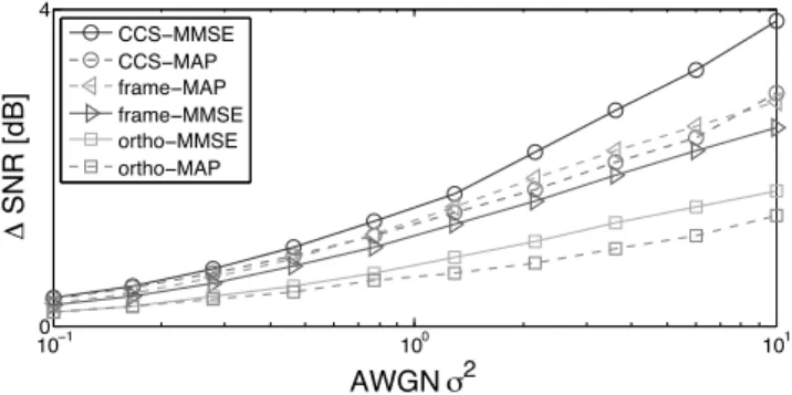
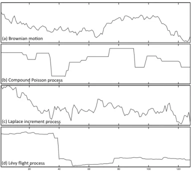
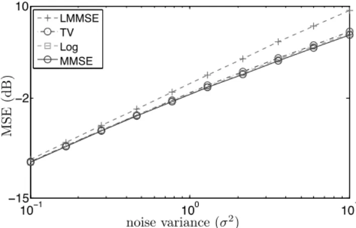
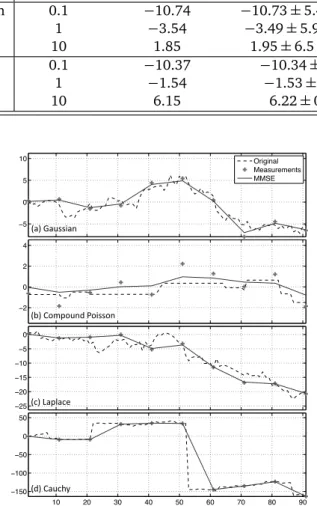
4.3.1 Lévy Processes . . . 41 4.3.2 Examples . . . 42 4.3.3 Innovation Modeling . . . 44 4.3.4 Measurement Model . . . 44 4.4 Bayesian Formulation . . . 45 4.4.1 MAP Estimation . . . 46 4.5 Message-Passing Estimation . . . 46 4.5.1 Exact Formulation . . . 46 4.5.2 Fourier-Domain Alternative . . . 48 4.5.3 Implementation . . . 49 4.6 Experimental Evaluation . . . 49 4.6.1 AWGN Denoising . . . 49 4.6.2 Signal Interpolation . . . 52

4.6.3 Estimation from Quantized Samples . . . 53

4.7 Summary . . . 54

5 Efficient Approximations to MMSE with Adaptive GAMP 55 5.1 Overview . . . 55 5.2 Introduction . . . 55 5.2.1 Related Literature . . . 57 5.3 Review of GAMP . . . 57 5.3.1 Sum-Product GAMP . . . 58 5.3.2 General GAMP . . . 59

5.3.3 State Evolution Analysis . . . 61

5.3.4 State Evolution Analysis for Sum-Product GAMP . . . 63

5.4 Adaptive GAMP . . . 64

5.4.1 ML Parameter Estimation . . . 65

5.4.2 Relation to EM-GAMP . . . 65

5.5 Convergence and Asymptotic Consistency with Gaussian Transforms . . . . 66

5.5.1 General State Evolution Analysis . . . 66

5.5.2 Asymptotic Consistency with ML Adaptation . . . 68

5.5.3 Computational Issues . . . 70

5.6 Identifiability and Parameter Set Selection . . . 70

5.6.1 Gaussian Mixtures . . . 71

5.6.2 AWGN output . . . 72

5.6.3 Initialization . . . 72

5.7 Experimental Evaluation . . . 72

5.7.1 Estimation of a Bernoulli-Gaussian input . . . 72

(15)

Table of Contents

5.8 Summary . . . 75

5.9 Appendix . . . 76

5.9.1 Convergence of Empirical Distributions . . . 76

5.9.2 Proof of Theorem 5.2 . . . 76 5.9.3 Proof of Theorem 5.3 . . . 81 5.9.4 Proof of Lemma 5.1 . . . 82 6 Numerical Evaluation 83 6.1 Introduction . . . 83 6.2 Compressive Sensing . . . 83 6.3 Image Deconvolution . . . 88 6.4 Discussion . . . 90

7 A Novel Nonlinear Framework for Optical Phase Tomography 93 7.1 Introduction . . . 93

7.2 Inhomogeneous Wave Equation . . . 94

7.3 Fourier Beam Propagation . . . 95

7.3.1 Derivation . . . 95

7.3.2 Implementation . . . 96

7.4 Iterative Reconstruction . . . 96

7.4.1 Derivation of the Gradient . . . 97

7.4.2 Recursive Computation of Gradient . . . 100

7.4.3 Iterative Estimation Algorithm . . . 100

7.5 Numerical Evaluation . . . 100 7.6 Summary . . . 102 8 Conclusions 103 8.1 Summary of Results . . . 103 8.2 Outlook . . . 104 Bibliography 107 Curriculum Vitæ 115

(16)

(17)

Chapter 1

Introduction

The terminverse problemrefers to a general framework used to convert observed ments into information about a physical object. For example, given tomographic measure-ments of a cell, we might wish to learn about its internal composition and structures. Hav-ing the capability to solve inverse problems is useful because it tells us somethHav-ing about physical quantities that we are unable to observe directly. Accordingly, inverse problems are some of the most important and well-studied mathematical problems in science and engineering. They have found many applications in different areas of science, including medical imaging, geophysics, astronomy, etc.

Two main reasons that make inverse problems of practical relevance difficult are as fol-lows:

– they are sometimes ill-posed, which means that many different solutions may be con-sistent with the measured data;

– they are high-dimensional in the sense that the measurements and the corresponding solution might contain millions or even billions of data entries.

These challenges force algorithmic solutions to strike a specific balance between the qual-ity of the reconstructed signal and the computational complexqual-ity for obtaining it. In this thesis, we attempt to refine the theory and develop new algorithms for addressing these challenges in a principled way. In particular, the ill-posed nature of the problem is offset by introducing a statistical framework where observed measurements are com-plemented with prior information on the statistics of the object. On the other hand, the high-dimensionality of the data is addressed by developing iterative algorithms that are re-stricted to performing the most basic operations with minimal memory and computational load. Nonetheless, as we shall see, our simple algorithms are still capable of producing satisfactory results for numerous practical applications in biomedical imaging.

1.1 Main Contributions

This thesis brings four main contributions to the field of inverse problems.

1. We provide a theoretical justification for the popular technique called cycle spinning in the context of general linear inverse problems. Cycle spinning has been extensively used for improving the visual quality of images reconstructed with wavelet-domain methods. We also refine traditional cycle spinning by introducing the concept of con-sistent cycle spinning that can be used to perform wavelet-domain statistical estima-tion. In particular, we empirically show that consistent cycle spinning achieves the minimum mean-squared error (MMSE) solution for denoising stochastic signals with sparse derivatives.

(18)

2. We introduce a continuous-domain stochastic framework for modeling signals with sparse derivatives. Our framework is based on Lévy processes and provides us with a large collection of structured statistical signals for benchmarking various standard algorithms used for solving inverse problems. We also develop a novel MMSE esti-mation algorithm for our signal model. This algorithm—based on a message-passing methodology—allows us to evaluate the optimality of other commonly used algo-rithms. For example, it is well known that the popular total variation (TV) method corresponds to performing maximum-a-posteriori (MAP) probability estimation of sig-nals with Laplace distributed gradients. One of our findings is that TV is in general a poor estimator for such Laplace processes; however, it reaches the performance of MMSE estimation for piecewise-constant compound Poisson processes.

3. Generalized approximate message passing (GAMP) is an iterative algorithm for per-forming statistical inference under generalized linear models. The algorithm can be derived by simplifying the equations of a more general belief propagation (BP) algo-rithm, which is intractable in the setting of general inverse problems. Our contribu-tion in the context of GAMP is twofold: (a) we extend the tradicontribu-tional GAMP with a novel algorithm called adaptive GAMP that can learn unknown statistical parameters present in the inverse problem during the reconstruction; (b) we prove that adaptive GAMP is asymptotically consistent for certain measurement models when learning is performed via the maximum-likelihood (ML) estimator. This means that adaptive GAMP can perform as well as the oracle algorithm that knows the parameters exactly. 4. We introduce a novel inverse problem formulation suitable for optical tomographic microscopy. The latter is an advanced digital imaging technique that combines the recording of multiple holograms with the use of inversion procedures to retrieve the quantitative information on the object. Here, our contribution is a nonlinear for-ward model that simulates the physics of the wave propagating through the sample. Compared to existing linear alternatives, our forward model provides an improved description of the measured data due to its ability to properly emulate the diffraction and propagation effects of the wave field. We finally develop a novel iterative algo-rithm, which uses the structure of our nonlinear forward operator, for quantitatively estimating the object.

1.2 Organization of the Thesis

This thesis is organized as follows: In Chapter 2, we expose the principles behind the formulation and resolution of inverse problems. We also present classical and state-of-the-art reconstruction techniques within a general statistical framework. In Chapter 3, we discuss an algorithmic strategy to perform competitive reconstruction using wavelet-regularization. The key concept that yields the improvements is cycle spinning, which we shall study in great detail. In Chapter 4, we study Lévy processes and the corresponding statistical estimators. The Lévy model will allow us to revisit several state-of-the-art re-construction algorithms and compare them against the optimal MMSE estimator that we develop. In Chapter 5, we present the adaptive GAMP algorithm that allows us to apply the message-passing philosophy to more general inverse problems. The algorithm has the capability to learn the unknown statistical parameters during the reconstruction. In Chap-ter 6, we present several numerical comparisons for algorithms discussed in the thesis. In Chapter 7, we present our algorithm for the optical tomographic microscope, which is a promising technique for quantitative three-dimensional (3D) mapping of the refractive index in biological cells and tissues.

(19)

Chapter 2

A Practical Guide to Inverse Problems

2.1 Introduction

In this chapter, we introduce the inverse problem formalism that will be used extensively in the sequel. We start by discussing several categories of forward models that can be used to model various practical acquisition systems. In the process, we also address the issues related to the discretization of continuous-domain inverse problems1_{. This is important}

since practical methods for solving inverse problems often rely on digital processing of the data in a computer. We finally introduce the statistical framework and several standard approaches that are currently used for solving inverse problems. Experimental evalua-tions throughout this chapter illustrate the capabilities of the described methods while simultaneously highlighting the necessity for the contributions presented in the rest of this thesis.

2.2 Forward Model

2.2.1 Continuous-Domain Formulation

The usual starting point in the formulation of inverse problems is the formal understand-ing of the acquisition process relatunderstand-ing the physical signal x to the measured data of the form

y=S_{x_}. (2.1)

The continuous-domain signalxmay be a function of space and/or time, while the mea-surements are stored in an M-dimensional vector y. For notational convenience, we as-sume that the signal and measurements are both real valued; nonetheless, all the al-gorithms considered in this thesis can be easily extended to work with complex valued signals. We also assume that the signal is of finite energy, and thus it belongs to the normed space L2(Rd). In full generality, the scalar value of x at every continuous

coor-dinater = (r1, . . . ,rd)inside Rd is denoted by x(r)∈R. We refer to S as theforward

operatorand typically assume that it models accurately the physics behind the acquisition. Depending on the acquisition modality, computation of S might involve various linear or nonlinear operations, including projection, orthogonal transformation, discretization, etc. In particular, we shall distinguish among the following four categories: nonlinear, generalized linear, linear, and signal denoising.

(20)

S

x(r) z y

H py|z(y|z)

Figure 2.1: Generalized linear model.

2.2.1.1 Nonlinear Models The most general nonlinear forward model allows us to handle so-phisticated acquisition modalities. Such models must still be sufficiently structured to be implemented and computed digitally on a computer. The computational complexity for numerical evaluation of such models should be weighted against the benefits of having a more accurate representation of the acquisition. As we shall see later, nonlinear models also complicate the recovery of the signal by leading to nonconvex costs in variational reconstruction methodology. In such difficult cases, it is beneficial to derive a lineariza-tions of the model. Then, one can use the latter to obtain a good initial guess for the solution that can subsequently be refined by using the nonlinear model. We will illustrate one concrete example of a nonlinear forward model in Chapter 7, where we consider the quantitative recovery of the refractive-index in tomographic microscopy[2].

2.2.1.2 Generalized Linear Models Thegeneralized linear model(GLM), illustrated in Figure 2.1, is a special case of nonlinear model that consists of a known linear mixing operator H followed by a probabilistic componentwise nonlinearitypy|z. Such models have been ex-tensively studied in statistics[3]. The linear part of the model has the general form

zm= [H{x}]m=

Z

Rd

x(r)ψ_m(r)dr_, (m=1, . . . ,M) (2.2) where the measurement functionψ_mrepresents the spatial response of themth detector in the acquisition system. The conditional probability distributionp_y_|_zthat is subsequently involved can model noise and various other types of deformations that are intrinsic to the physics of the acquisition.

One relevant practical example arises in analog-to-digital conversion (ADC), where one needs to estimate a signal from quantized measurementsy=Q(H_{x_}). This is a challeng-ing problem because the quantization function Q is nonlinear and the operator H mixes

x, thus necessitating joint estimation. Although reconstruction from quantized measure-ments is typically linear, more sophisticated, nonlinear techniques can offer significant improvements. In the case of ADC the improvement from replacing conventional linear estimation with nonlinear estimation increases with the oversampling factor[4–9]. From the algorithmic side, reconstruction methods based on GLM formulation might also suffer from nonconvexity of the cost function during optimization. The approaches based on message-passing algorithms seem to perform the best for GLM based inverse prob-lems. In Chapter 5, we will introduce adaptive generalized approximate message passing (adaptive GAMP) algorithm that is specifically tailored for statistical estimation under GLM[8–10].

2.2.1.3 Linear Models Further simplification of GLM is the linear forward model, which can be obtained by assuming that the distortion, characterized by the output nonlinearitypy|z, is additive and signal independent. This allows us to re-express (2.2) as

y=z+e with z=H_{x_}, (2.3)

where H is given in (2.2) ande represents the noise, which is very often assumed to be independent and identically distributed (i.i.d.) Gaussian. Linear inverse problems

(21)

2.2. Forward Model

are central to most modern imaging systems with applications in diverse areas such as biomicroscopy[11], magnetic resonance imaging[12], x-ray tomography[13], etc. The major advantage of linearity is that it allows us to borrow some intuition and rely on standard theoretical results from linear algebra. Typically, when confronted with a more general inverse problem, it is sensible that one reflects if there is a possibility to obtain a suitable linearization of the problem.

Most algorithms we develop in this thesis are particularly well-suited to solve linear in-verse problems under Gaussian noise assumption. It is possible to extend many of them to more general types of noise, but this might result in nonconvex formulation of the reconstruction. In such scenarios, we can use the solution obtained under the Gaussian assumption to initialize the more general algorithm.

2.2.1.4 Signal Denoising Even further simplification is possible by assuming that our acquisition system simply samples the signalx. In the context of the general form (2.2), this assumes thatψ_mcorresponds to a shifted Dirac delta function, which allows us to write

y=z+e with zm=x(rm), (m=1, . . . ,M) (2.4)

where_{r_m_}_m₌_1,...,_M _{are locations where the signal samples are taken and}_e_{represents the} noise. A more general denoising model with a signal dependent noise can be obtained by sampling directly in the GLM formulation.

Signal denoising is considered as the most basic form of signal reconstruction. The sources of noise are typically application dependent, but the two most common types are Gaussian and Poisson noises[14]. Algorithmically, signal denoising is useful as a key sub-routine in methods for solving more general inverse problems. As we shall see in detail, it is re-ferred to as proximal operator corresponding to a particular statistical distribution of the signal[15]. Also, denoising provides a practical scenario for testing various prior distribu-tions since it disregards the effects due to the linear mixing operator H. We shall consider the signal denoising problem in Chapter 4, where we study the optimal estimation of signals with sparse derivatives.

2.2.2 Discrete Representation of the Signal

It is most often impossible to solve an inverse problem analytically, and we must resort to a computer program to recoverx. In order to perform computations digitally, we need to discretizex into a finite number of parametersN that can be represented as a vectorx_∈

RN_{. To obtain a clean analytical discretization of the problem, we consider the generalized}

sampling approach usingshift-invariant reconstruction spaces [16]. The advantage of such a representation is that it offers the same type of error control as finite-element methods, i.e., the approximation error between the original signal and its representation in the reconstruction space can be made arbitrarily small by choosing a sufficiently fine reconstruction grid.

The idea is to represent the signal x by projecting it onto a reconstruction space. We define our reconstruction space at resolution∆as

V∆(ϕint)¬ ( x∆(r) = X k_∈Zd x[k]ϕ_int r ∆−k : x[k]_∈ℓ_∞(Zd) ) (2.5)

where x[k] ¬ _x(r)_|r₌k, andϕ_int is an interpolating basis function positioned on the

reconstruction grid∆Zd_{. The interpolation property is}ϕ_int(k) =δ[k]. For the represen-tation of x in terms of its samples x[k]to be stable and unambiguous, ϕ_int has to be a

(22)

valid Riesz basis forV∆(ϕint)[16]. Moreover, to guarantee that the approximation error

decays as a function of∆, the basis function should satisfy the partition of unity property X

k_∈Zd

ϕ_int(r₋k) =1, (2.6)

for allr_∈Rd_{. The projection of the signal onto the reconstruction space}_V_∆(ϕ_int)is given by PV∆x(r) = X k_∈Zd x(∆k)ϕ_int r ∆−k , (2.7)

with the property that PV∆PV∆x = PV∆x (i.e. PV∆x is a projection operator). To simplify

the notation, we shall use a unit sampling∆ =1 with the implicit assumption that the sampling error is negligible2. Thus, the resulting discretization is

x1(r) =PV1x(r) =

X

k_∈Zd

x[k]ϕ_int(r₋k). (2.8)

To summarize, x₁ is the discretized version of the original signal x and it is uniquely described by the samples x[k_{] =} _x₍r₎_|_r₌_k _fork_∈Zd_{. The main point is that the}

re-constructed signal is represented in terms of samples even though the problem is still formulated in the continuous-domain.

Although the signal representation (2.8) contains an infinite sum, in practice, we restrict ourselves to a subset ofNbasis functions withk_∈_Ω_{, where}_Ω_{is a discrete set of integer} coordinates in a region of interest (ROI). Hence, we rewrite (2.8) as

x1(r) = X

k_∈_Ω

x[k]ϕk(r), (2.9)

whereϕkcorresponds toϕ_int(· −k)up to modifications at the boundaries (periodization

or Neumann boundary condition).

2.2.3 Discrete Measurement Model

The discretization that we just presented allows us to obtain elegant discrete represen-tation for the generalized linear, linear, and signal denoising forward models. For more general nonlinear models the discrete representation might lack a closed form matrix-vector representation.

2.2.3.1 Generalized Linear Models By using the discretization scheme in (2.9), we are now ready to formally link the continuous model in Figure 2.1 to a corresponding discrete forward model. We substitute the signal representation (2.9) into (2.2) and obtain the discretized measurement model written in a matrix-vector form as

y_∼p_y_|_z(y_|z) with z=Hx, (2.10)

whereyis theM-dimensional measurement vector,x¬ _{_x[k]_}k_∈_Ω is theN-dimensional

signal vector, andHis theM×Nmeasurement matrix whose entry(m,k)is given by

[H]_m_,k ¬ 〈ψ_m,ϕk〉=

Z

Rd

ψ_m(r)ϕk(r)dr_. _(2.11)

This allows us to specify the discrete linear forward model that is compatible with the continuous-domain formulation. The solution of this problem yields the representation

x₁(r₎_of_x₍r₎_{which is parameterized in terms of the signal samples}_x_.

(23)

2.3. Statistical Inference

2.2.3.2 Nonlinear Models Unfortunately, in the case of nonlinear forward models, an elegant model similar to (2.10) is generally not possible. However, it is still necessary to represent the signal as in (2.9) and replace the forward operator S by a discrete operatorSthat can be computed by substituting continuous-domain operators with their discrete counterparts acting directly on the samplesx

y=S(x) +e, (2.12)

whereemodels the noise and potential discrepancies due to discretization. An example of such implementation is given in our microscopy application in Chapter 7.

2.2.4 Wavelet Discretization

Occasionally, we might prefer to represent the signal x in terms of its wavelet coeffi-cients [17]. In that case, we constrain the basis function ϕ_int to be a scaling function that satisfies the property of multiresolution[18]. To obtain an equivalent characteriza-tion of the object with its orthonormal wavelet coefficients, we simply define the wavelets as a linear combination ofϕk. Then, there exists a discrete wavelet transform (DWT)

represented with the matrixWthat bijectively mapsxto the wavelet coefficientswas

w=Wx _⇔ x=WTw, (2.13)

and that represents the signalxin a continuous wavelet basis. Note that the matrix-vector multiplications above have efficient filterbank implementations[19].

2.3 Statistical Inference

As we have mentioned in Chapter 1, inverse problems are often ill-posed. This means that measurementsycannot explain the signalxuniquely, and in order to separate meaningful solutions from the noise, we are obliged to introduce supplementary information describ-ingx. Statistical theory provides a unified approach for imposing additional constraints on the solution. The basic idea is to introduce a prior probability distributionpx favor-ing solutions that we consider to be correct and penalizfavor-ing those that we consider to be wrong. Then, given the priorpx, one can express the posterior distribution of the signal given the measurements

p_x_|_y(x_|y)_∝p_y_|_x(y_|x)p_x(x), (2.14) where_∝denotes equality after normalization, and py|x is the conditional distribution of the data given the signal. The posterior (2.14) provides a complete statistical characteri-zation to the problem. In particular, themaximum-a-posteriority(MAP) estimator is given by

b

xMAP ¬arg max x∈RN ¦ p_x_|_y(x_|y)© (2.15a) =arg min x∈RN ¦ −logpy|x(y|x) −log px(x) © (2.15b) =arg min x∈RN D(x) +φ(x) (2.15c)

In the context of inverse problems, the first term D in (2.15) is called the data term

due to its direct dependance on the measurements, while the second term φ is called theregularizerdue to its capability to impose more meaningful solutions. Similarly, we might be interested in finding theminimal mean squared error(MMSE) estimator, which

(24)

is usually expressed as the computationally intractableN-dimensional integral b

xMMSE ¬ arg min b x∈RN ¦ E_[_k_x₋_b_x_k2_|_y_]© _(2.16a) =E_[_x_|_y_] _(2.16b) = Z RN xpx|y(x|y)dx. (2.16c)

Once we accept the statistical perspective, we have several degrees of freedom to develop practical methods for solving inverse problems.

– The first degree of freedom lies in the specification of the prior distribution px. In some cases such as for MMSE estimation, we would want the prior to match the true empirical distribution of possible signalsxas closely as possible. At the same time, we want the prior to be as simple as possible in order to result in low-computation recon-struction algorithms. Prior distributions promotingsparsesolutions in some transform domains are currently state-of-the-art in this regard[20].

– Specification of the conditional distributionpy|xis the second issue to address. For the generalized linear model (2.10), this task becomes trivial and yields

p_y_|_x(y_|x) =p_y_|_z(y_|Hx) = M

Y

m=1

p_y_|_z(y_m_|[Hx]_m). (2.17) In more generic scenarios, one might either find an accurate statistical distribution characterizing the distortion or make a simplification by assuming a Gaussian noise model. The latter results in the popularleast-squaresdata term penalizing the quadratic distance betweenyandz.

– Once the priorpxand the data distributionpy|xare specified, we must develop an al-gorithm for computing the MAP, MMSE, or other estimators efficiently. We will cover several state-of-the-art approaches based on two distinct philosophies: (a) methods that explicitly minimize some predetermined cost-function, (b) methods based on pass-ing messages on graphical models. In the former category we have methods such as fast iterative shrinkage/thresholding algorithm (FISTA)[21]and alternating direction method of multipliers (ADMM) [22], while in the latter we have belief propagation (BP) algorithm[23]and generalized approximate message passing (GAMP)[24]. – Sometimes, we know the prior and the data distribution up to a finite number of

unknown parameters

px(x|θθθx), py|z(y|z,θθθz), (2.18) whereθθθ_x _∈ΘΘΘ_x andθθθ_z _∈ΘΘΘ_z represent parameters of the densities andΘΘΘ_x_⊆Rdx _and

Θ Θ

Θz ⊆ Rdz denote the corresponding parameter sets. For example, such scenario is realistic when we know the family of the prior distribution, but have no direct way of obtaining the parameters of the prior. Then, we must also find a method to choose the parametersθθθ_xandθθθ_zin a suitable way. The adaptive GAMP algorithm that we present in Chapter 5 is an effective method of doing this under generalized linear models. In the rest of this section, we will discuss some of the standard approaches for solving inverse problems.

2.4 Least Squares

The simplest prior is actually a flat prior. Thus, one basic approach for solving a general inverse problem is theleast-squares(LS) method that assumes a uniform priorpxand an

(25)

2.4. Least Squares

Algorithm 2.1: Gradient-descentto minimize:_CLS(x) = (1/2)_ky₋S(x)_k2 2

input: datay, initial guessbx0,

step-sizeγ_∈(0, 1/L], whereLis the Lipschitz constant of∇_C_LS, and efficient implementation of∇_CLS.

set: t←1 repeat

b

xt←bxt−1−γ∇_CLS(bxt−1) (gradient step)

t←t+1

untilstopping criterion return bxt

additive white Gaussian noise (AWGN)[25]. Although, it is particularly well suited for linear forward models withM_≥N, nothing prevents it from being applied more generally.

2.4.1 Nonlinear Model

In nonlinear form of LS, one seeks the solution b xLS ¬ arg min x∈RN CLS(x) (2.19a) =arg min x∈RN 1 2ky−S(x)k 2 2 , (2.19b)

which can be interpreted as a search for a signalxthat—by means of S—matchesy as closely as possible. The Euclidean norm_{k · k}2 in (2.19b) corresponds to the assumed

Gaussianity of the noise.

In the most general scenario, the LS functionCLS is non-convex, which implies that there might be many global and local solutions to the problem (2.19). In such cases, the com-putation of the global solution may be intractable, and we simply expect our optimization algorithms to find any one of the local minimizers of_CLS.

For differentiable forward modelsS, the gradient of_CLSis given by

∇_CLS₍_x_{) =}

_∂

∂_xS(x)

T

(S(x)₋y), (2.20)

where(∂_/∂_x₎_S₍_x₎_{is the Jacobian matrix of}_S_{. When the gradient (2.20) can be computed}

efficiently for allx, we can use the gradient descent method summarized in Algorithm 2.1 for finding a local solution of (2.19). The step-sizeγ >0 must be sufficiently small to guarantee the convergence of the algorithm. More specifically, for a Lipschitz continuous gradient∇_CLS

∇_CLS₍_x₎₋∇_CLS₍_z₎

2≤Lkx−zk2, (for allx,z∈RN) (2.21)

where L > 0 is the Lipschitz constant of∇_{CLS, the convergence is guaranteed for any}

γ_∈(0, 1/L][21, 26]. In practice, it might be difficult to determineLanalytically, and we might need to hand-pick a suitable step-sizeγ.

(26)

Algorithm 2.2: Gradient-descentto minimize: _CLS(x) = (1/2)_ky₋Hx_k2 2

Lipschitz constantL=λmax(HTH), and system matrixH.

set: t←1 repeat

bxt←bxt−1−(1/L)HT(Hbxt−1−y) (gradient step)

t←t+1

2.4.2 Linear Model

In the linear acquisition scenario, the LS reconstruction reduces to b xLS ¬arg min x∈RN CLS(x) (2.22a) =arg min x∈RN 1 2ky−Hxk 2 2 , (2.22b)

whereHis the measurement matrix given by (2.11). In this case, the gradient takes a simple form

∇_CLS(x) =HT(Hx−y). (2.23)

In imaging, due to high-dimensionality of the problem the matrices H andHT _cannot be stored explicitly in memory, and we require an efficient implementation of two basic operations:

1.

multiply

(x)¬ _Hx_, ₍_{for all}_x_∈RN₎

2.

multiplyTranspose

(z)¬ _HT_z_. ₍_{for all}_z_∈RM₎

Finding Lipschitz constant of the gradient reduces to computing the largest eigenvalue of HT_H

L=λmax(HTH), (2.24)

which can be precomputed once by using an iterative method such as power iteration. The iterative LS approach for linear models is summarized in Algorithm 2.2.

WhenM_≥NandHis nonsingular, the LS solution is given by bxLS=

HTH−1HTy (2.25a)

=x+HTH−1HTe (2.25b)

whereH−1_{denotes the inverse of the matrix} _H_{. In many practical applications, it is the}

case that H is ill-conditioned, which implies a presence of small singular values. As a result, LS yields a solution of poor quality due to the amplification of noise through the inverse ofHTHin (2.25b).

WhenM<N, the situation is worse, because anyx∈RN _{that satisfies}

HTHx=HTy, (2.26)

corresponds to a valid LS solution. Since in such scenarioHis singular, the system (2.26) has an infinity of possible solutions. Therefore, depending on the initial guessbx0_,

(27)

2.4. Least Squares

Algorithm 2.3: Fast gradient-descentfor: _CLS(x) = (1/2)_ky₋S(x)_k2 2

input: the datay, an initial guessbx0,

a step-sizeγ_∈(0, 1/L], whereLis the Lipschitz constant of∇_C_LS, and an efficient implementation of∇_CLS.

set: t←1,s0←bx0,k0←1 repeat b xt←st−1−γ∇_CLS(st−1) (gradient step) kt← 1₂ 1+p1+4k2_t₋₁ st ←bxt+ ((kt−1−1)/kt)(bxt−bxt−1) t←t+1

Algorithm 2.4: Fast gradient-descentfor: _CLS(x) = (1/2)_ky₋Hx_k2 2

Lipschitz constant L=λmax(HTH), and system matrixH.

set: t_←1,s0_←bx0,k0←1 repeat b xt←st−1−(1/L)HT(Hst−1−y) (gradient step) kt← 1₂ 1+p1+4k2_t₋₁ st ←bxt+ ((kt−1−1)/kt)(bxt−bxt−1) t←t+1

2.4.3 Signal Denoising

In signal denoising, LS returns the trivial solution

bxLS=y. (2.27)

This implies that to denoise a signal, we must go beyond the uniform prior.

2.4.4 Accelerated Gradient descent

It is well-known that the sequence of solutions_{bxt_}t∈Nobtained via the standard gradient

descent converges quite slowly to the local minimizer of the cost_CLS. In fact, it has been shown in[21]that its rate of convergence is given by

CLS(bxt₎_{− CLS}₍_x∗₎_≤ L

2tkbx

t₋_x∗_k2

2, (t>1) (2.28)

whereLis the Lipschitz constant of the gradient, andx∗_∈RN_{is any of the local}

minimiz-ers of_CLS.

It turns out, it is possible to obtain an algorithm that has exactly the same per-iteration complexity as the standard gradient-descent, but has significantly better rate of conver-gence. The idea was originally developed for differentiable functions by Nesterov in[27]. The improved rate of convergence comes from a controlled over-relaxation that utilizes

(28)

100 300 500 103

106 109

Gradient descend Fast gradient descend

100 300 500 0 10 20 (a) (b) (c) (d) iterations (t) iterations (t) LS cos t S NR (d B ) (e) (f)

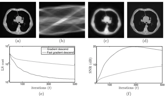
Figure 2.2: Least-squares reconstruction of a 256_×256 Lung image from 256 Radon measurements: (a) original; (b) measurements; (c) gradient-descent solution att=200; (d) fast gradient-descent solution at t =200; (e) evolution of the cost; (f) evolution of SNR

the previous iterates to produce a better guess for the next update. Possible implementa-tions of the scheme for LS are shown in Algorithms 2.3 and 2.4. The convergence rate of the accelerated gradient-descent is given by

CLS(bxt)_{− CLS}(x∗)_≤ 2L (t+1)2kbx

t

−x∗_k2₂. (t>1) (2.29)

In practice, switching from a linear to a quadratic convergence rate translates into impres-sive improvements over the standard gradient descent. Extensions of such accelerated techniques to non-smooth functions typically deliver state-of-the-art performance for high-dimensional inverse problems and will therefore constitute our methods of choice[21]. Figure 2.2 provides a concrete example where a linear inverse problem is solved with LS. ALungimage of size 256_×256 in Figure 2.2(a) is measured via 256 equally-spaced Radon projections in the range[₋π/2,π/2]in Figure 2.2(b). The measurements have addition-ally been corrupted by AWGN with the variance corresponding to 10 log₁₀(_kHx_k2_/_k_e_k2_{) =}

40 dB. Figures 2.2 (c) and (d) illustrate the solutions of Algorithms 2.2 and 2.4, respec-tively, after 200 iterations. The algorithms were initialized with the imagebx0 =0. Fig-ures 2.2(e) and (f) illustrate the evolution of the LS cost and the signal-to-noise-ratio (SNR) of the reconstruction, respectively. This example illustrates the convergence gain from using the accelerated gradient descent algorithm for LS. Moreover, it shows a typical behaviour of LS: as the algorithm progresses the quality of the recovered signal drops. The drop can be more or less significant depending on the amount of noise and the condition number of the measurement matrix. One standard approach to circumvent such behaviour at the reconstruction is to regularize the solution by replacing the uniform prior in LS with some otherpxthat imposes useful restrictions to the solution.

(29)

2.5. Wavelet-Domain Reconstruction

2.5 Wavelet-Domain Reconstruction

We now present wavelet-based methods for signal reconstruction. The idea is to define the prior distribution of the signal in the orthogonal wavelet domain. This is achieved by first expanding the signal as in (2.13), and introducing a simple prior for the wavelet coefficients. The prior distributions that we will consider have the general separable form

p_x(x)_∝p_w(Wx) = N

Y

n=1

p_w_n [Wx]_n, (2.30)

where ∝ denotes identity after normalization, and pwn is the distribution of the nth

wavelet-coefficient. We define the potential functionφ_was φw(w)¬ −log pw(w) (2.31a) =₋ N X n=1 logpwn(wn) = N X n=1 φwn(wn). (2.31b)

We start the section with the review of signal denoising, where we revisit the classical wavelet soft-thresholding algorithm[28]. The algorithm is based on two empirical obser-vations: (a) the energy of natural signals concentrates on very few wavelet coefficients; (b) the energy of i.i.d. noise is spread out uniformly in the wavelet domain. Accordingly, the noise can be suppressed by simply discarding small wavelet-coefficients. We then ex-tend the wavelet denoising algorithm to more general inverse problems by introducing the concept of proximal operators. Initially, we will limit our discussion to the linear forward models with AWGN. At the end of the section, we present a more general algorithm for computing wavelet-based solutions under nonlinear forward models.

2.5.1 Signal Denoising

In the simplest case of AWGN denoising, the posterior distribution of the signal becomes

p_x_|_y(x_|y)_∝ N Y n=1 G(x_n₋y_n;σ2)p_w_n([Wx]_n), (2.32) where_G denotes the zero-mean Gaussian distribution

G(x;σ2₎_¬ 1

σp2πe

−2xσ22_. _(2.33)

The orthonormality of the wavelet-basis implies the norm identity _kx_k2

2 = kWxk 2 2 that

allows for an equivalent wavelet-domain characterization of the signal statistics

p_w_|_u(w_|u)_∝ N Y n=1 G(w_n₋u_n;σ2)p_w_n(w_n), (2.34) wherew=Wxandu=Wy. Such characterization effectively reduces the vector estima-tion problem intoN-scalar estimation subproblems.

2.5.1.1 MAP Denoising The wavelet–based MAP estimator is given by b

xMAP=arg min x∈RN CMAP(x) (2.35a) =arg min x∈RN 1 2kx−yk 2 2+σ 2_φ w(Wx) (2.35b) (a) =WTarg min w∈RN 1 2kw−Wyk 2 2+σ 2_φ w(w) , (2.35c)

(30)

where in (a) we use the orthonormality of the wavelet-basis. Computationally, the esti-mator (2.35) reduces to

– wavelet-transformationu=Wy, – scalar MAP estimation

b wn=arg min w∈R ₁ 2(w−un) 2₊_σ2_φ wn(w) , (n=1, . . . ,N) (2.36) – inverse wavelet-transformationbxMAP=WTwb.

Since, the scalar estimator (2.36) can be precomputed and stored in a lookup table, the overall denoising procedure is very efficient. The optimization in (2.35c) can be repre-sented more compactly by defining theproximal operator

b w=prox_φ w u;σ2 (2.37a) =     prox_φ_w 1(u1;σ 2₎ .. . proxφ_wN(uN;σ2)     (2.37b) ¬ _{arg min} w∈RN 1 2kw−uk 2 2+σ 2_φ w(w) . (2.37c)

Then wavelet-domain MAP estimation can be represented with a simple and efficient for-mula

b

xMAP=WTproxφw(u;σ

2₎ _with _u₌_Wy_. _(2.38)

2.5.1.2 MMSE Denoising The wavelet-based MMSE estimator can be computed in a similar way by performing the following operations

– wavelet-transformationu=Wy, – scalar MMSE estimation

b wn= Z R wnpwn|un(wn|un)dwn, (n=1, . . . ,N) (2.39a) = R RwnG(wn−un;σ 2₎_p wn(wn)dwn R RG(wn−un;σ 2₎_p wn(wn)dwn , (2.39b)

– inverse wavelet-transformationbxMMSE=WTwb. This can be represented more compactly as

b

xMMSE=W T_E

w|u[w|u] with u=Wy. (2.40)

A quick glance at (2.40) and (2.38) reveals major similarities between MMSE and MAP estimators. The only observable difference is the shape of the scalar estimation functions: in MMSE they are obtained via integration (2.39), while in MAP they are obtained via optimization (2.36). Unfortunately, this similarity is restricted to signal denoising with orthogonal wavelets, and breaks for more general forward models and priors. Orthonor-mality of the wavelet transform and Parseval’s norm identity provide the necessary ele-ments for making MMSE computationally equivalent to MAP. One of our contributions in Chapter 3 will be the extension of this idea to more general wavelet-transforms by relying on the concept of consistent cycle spinning.

(31)

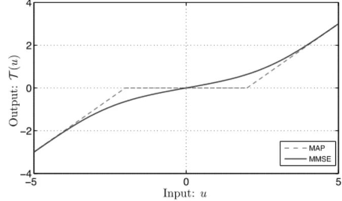
2.5. Wavelet-Domain Reconstruction −5 0 5 −4 −2 0 2 4 Input O u tp u t MAP MMSE Output: T ( u )

Figure 2.3: Illustration of TMAP (dashed) and TMMSE (solid) shrinkage functions for a Laplace prior with parameterλ=2 and AWGN of varianceσ2₌_1.

2.5.1.3 Illustrative Examples As the first example, we assume that the wavelet-coefficients of the signal are zero-mean i.i.d. Gaussian with varianceσ2_x. Since the wavelet-expansion of an i.i.d. Gaussian vector has exactly the same distribution, estimation can be performed in the spatial- or the wavelet-domains equivalently. By introducing the prior distribution

pw(w;σ2x) = 1 p (2πσ2₎Ne −k₂wσk22 x , (2.41)

into (2.36) and (2.39), we obtain b wMAP=wbMMSE= σ2 x σ2 x+σ2 u. (2.42)

The estimation is thus reduced to linearlyshrinkingnoisy wavelet-coefficientsuin a way that is inversely proportional to signal powerσ2

x and proportional toσ2, i.e., higher noise implies more shrinking.

When the wavelet-coefficients of the signal are assumed to be i.i.d. Laplace random vari-ables with parameterλ, the prior is given by

pw(w;λ) = λ 2e

−λkwk1_. _(2.43)

Then, MAP estimator reduces to b

xMAP=W T

TMAPWy;λσ2, (2.44)

where the pointwise soft-thresholding function_T is given by

TMAP(w;λ)¬ ₍_|_w_{| −}_λ₎₊_sgn₍_w₎_. _(2.45)

The resulting denoising method corresponds to the popular wavelet-domain soft-thresholding algorithm that yields sparse solutions[28, 29]. The scalar MMSE estimator_TMMSEfor the Laplace prior has also an analytical expression, albeit a more complicated one, that can easily be found in the literature[15]. The final MMSE estimator is then computed as

b

xMMSE=W T

TMMSEWy;λ,σ2, (2.46)

(32)

Algorithm 2.5: ISTAto minimize: _CMAP(x) = (1/2)_ky₋Hx_k2

2+σ2φw(Wx) input: datay, initial guessbx0,

Lipschitz constantL=λmax(HTH), noise varianceσ2, system matrixH, and operator proxφw.

set: t←1 repeat zt ←bxt−1−(1/L)HTHbxt−1−y (gradient step) bxt←WTproxφw(Wz t_;_σ2_/_L₎ _{(shrinkage step)} t←t+1

2.5.2 Linear Model

We now consider the linear inverse problem

y=Hx+e, (2.47)

where the vectorerepresents i.i.d. Gaussian measurement noise of variance σ2_{. Given}

the wavelet-domain prior (2.30), one can express the posterior distribution

p_x_|_y(x_|y)_∝p_y_|_x(y_|x)p_x(x) (2.48a) ∝ M Y m=1 G(y_m₋[Hx]_m;σ2) N Y n=1 p_w_n [Wx]_n, (2.48b)

where_G is the Gaussian distribution. MAP estimator is given by b

xMAP=arg min x∈RN CMAP(x) (2.49a) =arg min x∈RN ₁ 2ky−Hxk 2 2+σ 2_φ w(Wx) , (2.49b)

whereφ_w is the potential function in (2.31). Although, we might also be interested in finding the MMSE solution to general linear forward models, this becomes computation-ally intractable. We will thus concentrate in obtaining a method for computing the MAP estimator (2.49). In Chapter 5, we will return to the problem of MMSE estimation and present an adaptive GAMP method that can be used for approximating MMSE.

2.5.2.1 ISTA Algorithm An elegant and nonparametric method for computing the estimator (2.49) is the so-called iterative shrinkage/thresholding algorithm (ISTA) [30–32]. The latter relies on the separable proximal operator

b w=prox_φ w(u;λ) ¬_{arg min} w∈RN 1 2kw−uk 2 2+λφw(w) . (2.50a)

The proximal operator corresponds to the wavelet-based MAP solution of the denoising problem (2.37). For our wavelet-domain priors, it reduces to a collection of scalar nonlin-ear maps that can be precomputed and stored in a lookup table.

Based on the definition of our forward model, ISTA can be expressed as in Algorithm 2.5. Iterations of ISTA combine gradient-descent steps with pointwise proximal operators. To

(33)

2.5. Wavelet-Domain Reconstruction

Algorithm 2.6: FISTAfor:_CMAP(x) = (1/2)_ky₋Hx_k2

2+σ2φw(Wx) input: datay, initial guessbx0,

Lipschitz constant L=λmax(HTH), noise varianceσ2, system matrixH, and operator proxφw.

set: t←1,s0←bx0,k0←1 repeat zt←st−1−(1/L)HT(Hst−1−y) (gradient step) b xt←WTproxφw(Wz t_;_σ2_/_L₎ _{(shrinkage step)} k_t_← 1 2 1+p1+4k2 t−1 st _←_b_xt_{+ ((}_k t−1−1)/kt)(bxt−bxt−1) t_←t+1

understand why the algorithm actually minimizes the cost, we bound_CMAPas follows CMAP(x) = 1 2kHx−yk 2 2+σ 2_φ w(Wx) (2.51a) (a) =1 2kHbx t−1₋_y_k2 2+ (x−bx t−1₎T_HT₍_H_b_xt−1₋_y₎ _(2.51b) + (x₋bxt−1)THTH(x₋bxt−1) +σ2φ_w(Wx) (b) ≤1₂kHbxt−1₋y_k2₂+ (x₋bxt−1)THT(Hbxt−1₋y) (2.51c) + 1 2γkx−bx t−1_k2 2+σ 2_φ w(Wx) = 1 2γ x₋bxt−1₋_γ_HT_H_b_xt−1₋_y 2 2+σ 2_φ w(Wx) +const (2.51d) =_Q(x,bxt−1), (2.51e)

where “const” denotes terms that are constant with respect tox. In (a) we performed a quadratic Taylor expansion of the cost aroundx=bxt−1, in (b) we selectedγsuch that

1 2γkxk 2 2≥ kHxk 2 2 (2.52)

for allx∈RN_{. To guarantee monotone convergence, equation (2.52) restricts the choice}

ofγto the interval(0, 1/L], where L=λmax(HTH). Note that the auxiliary cost function Q(x,bxt−1₎_{that depends on the previous estimate}_b_xt−1_{is much simpler than the original}

cost_CMAP. Our formulation imposes_Q(x,bxt−1₎_{≥ CMAP}₍_b_xt−1₎_{with equality when}_x₌_b_xt−1_.

Thus, one can recover the ISTA iteration by simply minimizing the cost_Q(x,bxt−1₎_over_x

and setting the solution to bebxt_.

2.5.2.2 FISTA Similar to the gradient descent algorithm for LS estimation, the main weakness of ISTA is in its slow convergence. FISTA, summarized in Algorithm 2.6, is an improvement of the standard ISTA that results in a rate of convergence that is equivalent to accelerated gradient descent of Section 2.4.4. The convergence to the global minimizer ofCMAPis only achieved when the potential functionφ_wis convex[21]. Note that a simpler, and in some cases more effective way of speeding up ISTA, was proposed by Wrightet al.[33], where the acceleration is obtained by using larger step-sizes.