Czado, Min:
Testing for zero-modification in count regression
models
Sonderforschungsbereich 386, Paper 474 (2006)
Online unter: http://epub.ub.uni-muenchen.de/
Testing for zero-modification in count
regres-sion models
Claudia CZADO and Aleksey MIN1
Center for Mathematical Sciences Munich University of Technology
Boltzmannstr. 3 D-85747 Garching, Germany
Abstract
Count data often exhibit overdispersion and/or require an adjustment for zero out-comes with respect to a Poisson model. Zero-modified Poisson (ZMP) and zero-modified generalized Poisson (ZMGP) regression models are useful classes of models for such data. In the literature so far only score tests are used for testing the neces-sity of this adjustment. For this testing problem we show how poor the performance of the corresponding score test can be in comparison to the performance of Wald and likelihood ratio (LR) tests through a simulation study. In particular, the score test in the ZMP case results in a power loss of 47% compared to the Wald test in the worst case, while in the ZMGP case the worst loss is 87%. Therefore, regardless of the computational advantage of score tests, the loss in power compared to the Wald and LR tests should not be neglected and these much more powerful alternatives should be used instead. We also prove consistency and asymptotic normality of the maximum likelihood estimators in the above mentioned regression models to give a theoretical justification for Wald and likelihood ratio tests.
Keywords: generalized Poisson distribution; likelihood ratio test; maximum likeli-hood estimator; overdispersion; score test; Wald test; zero-modification
1Corresponding author.
Fax: +49/89/289-17435
1
Introduction
Zero-inflated generalized Poisson (ZIGP) regression models have recently been found useful for the analysis of count data with a large amount of zeros ( see e.g. Famoye and Singh (2003), Gupta et al. (2004), Joe and Zhu (2005), Bae et al. (2005) and Famoye and Singh (2006)). It is a large class of regression models which contains zero-inflated Poisson (ZIP), generalized Poisson (GP) and Poisson regressions (Mul-lahy (1986), Lambert (1992), Consul and Famoye (1992) and Famoye (1993)). The interest in this class of regression models is driven by the fact that it can handle overdispersion and/or zero-inflation which count data very often exhibit.
Score tests are widely used for testing misspecifications in count regression mod-els because they require to fit the model only under the null hypothesis. In partic-ular, van den Broek (1995) proposed a score test for testing zero-inflation in ZIP regression and Gupta et al. (2004) derived score tests for testing zero-inflation or overdispersion in ZIGP regression. The score test for zero-inflation considered by the above authors is as they noted the score test for zero-inflation or zero-deflation, i.e. for zero-modification in zero-modified Poisson (ZMP) regression (see Dietz and B¨ohning (2000)) and zero-modified generalized Poisson (ZMGP) regression. In order to derive a score test only for zero-inflation, the problem of testing parameters on the boundary of the parameter space needs to be addressed. Consequently, the lim-iting distribution of the score statistic will differ from a standard χ2−distribution. For insightful discussions on this problem we would like to refer to Verbeke and Molenberghs (2003).
Nowadays, given modern computing power, the computational advantage of score tests has lost some of its original attractivity in many problems. Therefore we think that more attention should be paid to Wald and likelihood ratio (LR) tests for ZMP and ZMGP regressions. The objective of this paper is to derive the appropriate asymptotic theory for the ZMGP regression models and to investigate the performance of Wald, LR and score tests for testing modification, i.e. zero-inflation or zero-deflation. Our theoretical results also remain valid for GP and ZMP regression models subject to appropriate changes in assumptions.
There is also a count regression for overdispersed and zero-inflated data based on a negative binomial (NB) distribution. This is a zero-inflated negative binomial (ZINB) regression (see Ridout et al. (2001) and Hall and Berenhaut (2002)). It is not a subject of the paper but we list most important differences, from our point of view, between regression models based on a NB and GP distributions in next sections.
In Section 2 we introduce the GP distribution and discuss its basic forms and properties. A ZMGP regression model is defined in Section 3. Section 4 gives the asymptotic existence, the consistency and the asymptotic normality of the ML estimator in a ZMGP regression model. In Section 5 we compare the performance of the score test for detecting zero-modification in ZMP and ZMGP models to the
performance of the Wald and LR tests in a simulation study. In particular it is shown that using the score test one may lose in test power compared to the Wald test up to 47% for the ZMP case and up to 87% for the ZMGP case. We also illustrate that the score test for zero-modification in the analysis of the apple propagation data (see Ridout and Dem´etrio (1992)) does not always detect zero-modification while the Wald and LR tests give strong evidence for zero-modification. Thus the score test can result in misleading conclusions about the presence of zero-modification. The Fisher information matrix of the ZMGP regression and the proof of Theorem 1 is given in the Appendix.
2
The GP distribution
A random variable ˜Y is said to be distributed according to a GP distribution with parameters µand ϕ, which we denote byGP(µ, ϕ), if its probability mass function is given by
Pµ,ϕ(y) := (
µ(µ+y(ϕ−1))y−1ϕ−ye−(µ+y(ϕ−1))/ϕ/y! fory= 0,1, . . .
0 fory > m, when ϕ <1. (1)
The real-valued parametersµandϕare assumed to satisfy the following constraints:
• µ >0;
• ϕ≥max{1/2,1−µ/m}, wherem (m≥4) is the largest natural number such that µ+m(ϕ−1)>0 when ϕ <1.
If ϕ < 1 then (1) does not correspond to a probability distribution. However the lower limit, imposed onϕin this case, guarantees us that the total error of truncation is less than 0.5% (see Consul and Shoukri (1985)). Since all discrete distributions are truncated under sampling procedures this is found to be a quite reasonable condition.
The GP distribution was first introduced by Consul and Jain (1970) and sub-sequently studied in detail by Consul (1989). One particular property of the GP distribution is that the variance of this distribution is greater than, equal to or less than the mean according to whether the second parameter ϕ is greater than, equal to or less than 1. More precisely (for details see Consul (1989), page 12 ), if
˜
Y ∼GP(µ, ϕ) then the mean and variance ofY are given by
E( ˜Y) = µ (2)
and
A NB distribution with meanµand overdispersion parametera >0 (see Lawless (1987) for precise definition) also has a flexible variance function. Its variance is given by µ(1 +aµ). Thus the overdispersion in the GP case is independent of the mean while this is not the case for the NB distribution. This implies that overdispersion in the NB case might be present over and above that accounted for by
a; a fact concurred by Lawless (1987). Czado and Sikora (2002) also noted this and developed an approach based on p−value-curves to quantify overdispersion effects more precisely. Another significant difference between these two distributions is that the NB distribution belongs to the exponential family whenever the overdispersion parameterais known while this does not hold for the GP distribution. A comparison of GP and NB probability functions can be found in Joe and Zhu (2005) and Gschl¨oßl and Czado (2005).
There is a form of the GP distribution obtained by assuming that ϕ−1 is linearly proportional to µ, say ϕ−1 =αµ for α >0. In the literature it is known as a restricted generalized Poisson (RGP) distribution (see Consul (1989), p. 5) and the relation between its mean and variance is given byV ar( ˜Y) = (1+αE( ˜Y))2E( ˜Y). Thus overdispersion in the RGP case is not independent of the mean. To avoid the point indicated in the previous paragraph we deal here only with an unrestricted form (1) of the GP distribution.
3
ZMGP regression
A ZMGP distribution is defined analogous to a ZMP distribution (see Dietz and B¨ohning (2000)) and its probability mass function is given by
Pµ,ϕ,ω(y) :=P(Y =y) = (
ω+ (1−ω)P( ˜Y = 0) y= 0,
(1−ω)P( ˜Y =y) y= 1,2, . . . , (4)
where ˜Y is distributed according to the GP distribution with parameters ϕ and µ
and the parameterω satisfies the following restriction
−exp(−µ/ϕ)
1−exp(−µ/ϕ) ≤ω ≤1. (5)
Thus, this distribution has 3 parametersµ, ϕand ω and will be further denoted by
ZM GP(µ, ϕ, ω).
The above condition (5) ensures that (4) defines a probability mass function for negative values ofωcorresponding to zero-deflation. Positive values of the parameter
ω correspond to zero-inflation which mostly occurs in practice. In this case ω is a probability of zero outcome of a zero-inflating Bernoulli distribution.
A simple calculation using equations (2) and (3) imply that the mean and vari-ance of the ZMGP distribution are given by
and
V ar(Y) = E(Y) ϕ2+µω
. (7)
One of the main benefits of considering a regression model based on the ZMGP distribution is that it gives a large class of regression models for count response data. In particular, it reduces to Poisson regression when ϕ= 1 and ω= 0, to GP regression when ω = 0 and to ZMP regression when ϕ = 1. Moreover, by virtue of (6) and (7) this regression can be used to fit zero-modified count regression data exhibiting overdispersion or underdispersion.
Analogous to the generalized linear models (GLM) framework, we now intro-duce a regression model with response Yi and (known) explanatory variables xi =
(xi0, xi1, . . . , xip)t withxi0 = 1 fori= 1, . . . , n: 1. Random components:
{Yi, 1≤i≤n} are independent whereYi∼ZM GP(µi, ϕ, ω).
2. Systematic components:
The linear predictors ηi(β) =xtiβ for i= 1, . . . , n influence the responseYi.
Here β= (β0, β1, . . . , βp)t is a vector of unknown regression parameters. The
matrix X= (x1, . . . ,xn)t is called the design matrix. 3. Parametric link components:
The linear predictors ηi(β) are related to the parameter µi of Yi by µi =
exp(ηi(β)) fori= 1, . . . , n.
Here and in the subsequent sections, At andat denote the transpose of a matrixA and a vector a, respectively. To stress the fact that the distribution of the responses Yi’s does not belong to the exponential family, this regression will be called the
ZMGP regression model. It should be noted that parameter ϕ and ω are assumed to be constant and (5) now should hold for allµi,i= 1,2, . . . , n. Further, we denote
the joint vector of the regression parameters β and the parameters ϕand ω of the ZMGP distribution by δ, i.e. δ := (βt, ϕ, ω)t, and its ML estimator by ˆδ.
The following abbreviations fori= 1, . . . , nwill be used throughout in the paper:
µi(β) := exp xtiβ
, fi(β, ϕ) := exp (−µi(β)/ϕ),
gi(δ) := ω+ (1−ω)fi(β, ϕ) =Pµi(β),ϕ,ω(0).
can be written as ln(δ) = n X i=1 1l{yi=0}log (gi(δ)) + n X i=1 1l{yi>0} log(1−ω) +xt iβ− 1 ϕµi(β) + (yi−1) log [µi(β) +yi(ϕ−1)] −yilogϕ−yi 1 ϕ(ϕ−1)−log(yi!) .
Further the score vector, i.e. the vector of the first derivatives, has the following representation: sn(δ) = (s0(δ), . . . , sp(δ), sp+1(δ), sp+2(δ))t, (8) where sr(δ) := ∂ln(δ) ∂βr = n X i=1 sr,i(δ) with sr,i(δ) := −xir1l{yi=0} (1−ω)fi(β, ϕ)µi(β) ϕgi(δ) + xir1l{yi>0} 1 + µi(β)(yi−1) µi(β) + (ϕ−1)yi − µi(β) ϕ (9) forr = 0, . . . , p, sp+1(δ) := ∂ln( δ) ∂ϕ = n X i=1 sp+1,i(δ) with sp+1,i(δ) := 1l{yi=0} (1−ω)fi(β, ϕ)µi(β) ϕ2g i(δ) + 1l{yi>0} yi(yi−1) µi(β) + (ϕ−1)yi − yi ϕ + µi(β)−yi ϕ2 (10) and sp+2(δ) := ∂ln( δ) ∂ω = n X i=1 sp+2,i(δ) with sp+2,i(δ) := 1l{yi=0} 1−fi(β, ϕ) gi(δ) − 1l{yi>0} 1 1−ω, (11) fori= 1, . . . , n.
4
Asymptotic theory
Fahrmeir and Kaufmann (1985) proved consistency and asymptotic normality of the ML estimator in GLM for canonical as well as noncanonical link functions under mild assumptions. Their method can be adapted for proving similar results for the ZMGP regression.
As in Fahrmeir and Kaufmann (1985), we use the Cholesky square root matrix for normalizing the ML estimator. The left Cholesky square root matrix A1/2 of a positive definite matrix A is the unique lower triangular matrix with positive diagonal elements such that A1/2 A1/2t = A (see Stewart (1998), p. 188). For convenience, set At/2 := A1/2t, A−1/2 := A1/2−1
and A−t/2 := At/2−1
. In this paper we deal only with the spectral norm of square matrices denoted by k · k. The spectral norm of a real-valued matrix Ais given by
kAk= maximum eigenvalue of AtA1/2
= sup
kuk2=1
kAuk 2,
wherek · k2 denotes theL2– norm of vectors. We drop subindex 2 ink · k2 since the spectral norm is generated by the L2–norm of vectors and arguments of considered norms are always clearly defined. The minimal eigenvalue of a square matrix A will be further denoted by λmin(A) and the vector of true parameter values of the
ZMGP regression will be denoted as δ0. Further Fn(δ) will stand for the Fisher
information matrix in a ZMGP regression evaluated at δ. It should be noted that the entries of the Fisher information matrix in a ZMGP regression have a closed form (see Appendix) while this is not the case in regression models associated with a NB distribution (see e.g. Lawless (1987)).
Now denote a neighborhood of δ0 by
Nn(ε) ={δ :kFt/n2(δ0)(δ−δ0)k ≤ε} (12) forε >0.
For convenience, we drop the argumentsδ0,β0andϕ0 as well as the subindexδ0 in µi(β0),fi(β0, ϕ0),gi(δ0),Pδ0, Eδ0 etc. and write µi, fi, gi, P, E etc. Constants will be further denoted by C and c, with subindexes or without them. They may depend onδ0but not onn. The sameC’s andc’s in different places denote different constants. Finally, the n-dimensional unit matrix will be denoted by In and an admissible set for a vector β of regression parameter will be denoted byB.
We make the following assumptions. (A1)
n λmin(Fn) ≤
C1 ∀ n≥1, where C1 is a positive constant.
(A3) Assume that B ⊂ Rp+1 is an open set and δ
0 is an interior point of the set Kδ :=B×Φ×Ω, where Φ := [1,∞) and Ω := [−cω,1]. Here cω is a positive
constant such that (5) holds for all x∈Kx, β∈B and ϕ∈Φ.
Now we state our main result which is the analogue to Theorem 4 of Fahrmeir and Kaufmann (1985).
Theorem 1. Under the assumptions (A1)–(A3), there exists a sequence of random
variables ˆδn, such that
(i) P(sn(ˆδn) = 0)→1 as n→ ∞ (asymptotic existence), (ii) δˆn−→P δ0 as n→ ∞ (weak consistency),
(iii) Ft/n2(ˆδn−δ0)=D⇒Np(0,Ip+3) as n→ ∞ (asymptotic normality). Remarks
(i) Assumption (A1) is more restrictive than the corresponding condition (D) of Fahrmeir and Kaufmann (1985). Assumption (A2) means that we deal with compact regressors.
(ii) If δ0 lies on the boundary of parameter space Kδ, i.e. (A3) is violated, then
statements of Theorem 1 do not hold anymore. Particularly this implies that we cannot test the adequacy of the GP regression. However the asymptotic results of Theorem 1 remain valid in GP or ZMP regression models subject to appropriate changes to be performed in the log-likelihood, the ML equations and the Fisher information matrix as well as in Assumption (A3).
(iii) We would like to especially note that ω = 0 is not on the boundary of the parameter space in ZMGP and ZMP regression models, thus allowing for a direct application of Wald, LR and score tests.
5
Applications
5.1
Power comparison of score, Wald and LR tests in
ZMP and ZMGP models
Jansakul and Hinde (2002) investigated the performance of the score test for zero-inflation in small and moderate sample sizes within the ZIP regression model. They noted that their score test compares the Poisson model to the ZMP model thus avoiding the problem of testing on the boundary of zero-inflation.
By virtue of Remarks (ii) and (iii) of Theorem 1, we can construct the Wald and LR tests for testing zero-modification in ZMP models and then compare their perfor-mance with the perforperfor-mance of the score test. Note this comparison is only feasible
for models with a constant zero-modification parameter. In particular, Jansakul and Hinde (2002) considered models with ω = 0,0.25,0.45 and linear predictors
ηi(β) = 0.25,0.75 and ηi(β) = 0.75−1.45xi for i= 1, . . . , n and n= 50,100,200.
Covariates xi’s were taken uniformly from (0,1). For each combination of sample
size and model they simulated 1000 sets of responses from the working model. The simulation setup for the constant linear predictorsηi’s implies that the corresponding
Poisson distribution has approximately 28% ( ηi(β) = 0.25) and 12% (ηi(β) = 0.75)
of zero responses. In the case of nonconstant linear predictors, the probability of obtaining zero outcomes from the Poisson distribution with parameter exp(ηi(β))
varies between 0.12 and 0.61 for i = 1, . . . , n. We used their simulation setup to compare the performance of the three above mentioned tests in S-PLUS 7.0 on a Windows platform. The ML estimators were determined with a help of the S-PLUS function ”nlminb” which finds the minimum of a smooth nonlinear function subject to bound-constrained parameters.
The Wald statistic for testing H0 : ω = 0 versus H1 : ω 6= 0 has the following form Wω = ˆ ω2 ˆ σ2 ω ,
where ˆω is the ML estimator of ω in a ZMP regression and ˆσ2
ω is the estimated
variance of ˆω, which is the corresponding diagonal element of the inverse of the Fisher information matrix evaluated at (ˆω,βˆ). The LR statistic for the same testing problem is given by LRω =−2(lPn(ˆβ P )−lZMP n (ˆδ ZMP )), wherelP n(·) and ˆβ P
denote, respectively, the log-likelihood and the ML estimator in a Poisson regression model,lZMP
n (·) and ˆδ
ZMP
= ( ˆβZMP,ωˆZMP
) denote, respectively, the log-likelihood and the ML estimator in a ZMP regression model. The score statistic for the above testing problem is derived in detail by Jansakul and Hinde (2002) and therefore it is not given here. Further following them, the score statistic is denoted by Sω.
Estimated upper tail probabilities for anαsize test are computed by calculating the proportion of times whenWω,LRωorSωare greater than or equal to the critical
value χ21,1−α. For the Wald test we have for example
#{j:Wωj ≥χ12,1−α, j= 1, . . . ,1000}
1000 .
Hereχ2
1,1−α is the (1−α)100% quantile of aχ2distribution with 1 degree of freedom
and Wωj denotes the value of Wω in thej−th sample. Note that when samples are
drawn from the Poisson distribution the estimated upper tail probabilities corre-spond to the estimated level of the test. For ZMP samples with zero-modification
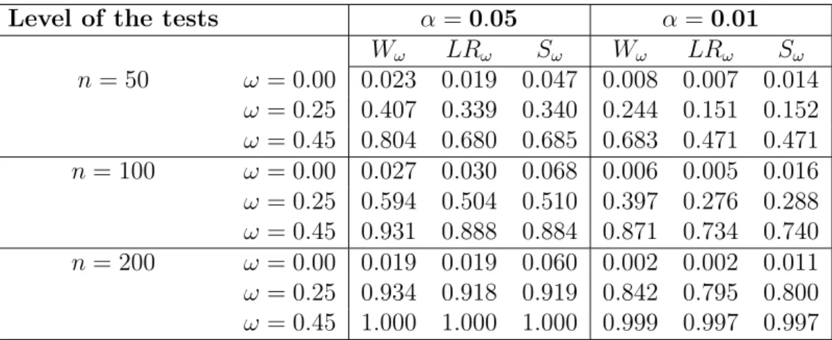
Table 1: Estimated upper tail probabilities for Wald (Wω), LR (LRω) and score (Sω)
statistics at χ2
1,1−α based on 1000 samples from the ZMP model with nonconstant linear
predictorsηi(β) = 0.75−1.45xi
Level of the tests α =0.05 α=0.01
Wω LRω Sω Wω LRω Sω n= 50 ω = 0.00 0.023 0.019 0.047 0.008 0.007 0.014 ω = 0.25 0.407 0.339 0.340 0.244 0.151 0.152 ω = 0.45 0.804 0.680 0.685 0.683 0.471 0.471 n= 100 ω = 0.00 0.027 0.030 0.068 0.006 0.005 0.016 ω = 0.25 0.594 0.504 0.510 0.397 0.276 0.288 ω = 0.45 0.931 0.888 0.884 0.871 0.734 0.740 n= 200 ω = 0.00 0.019 0.019 0.060 0.002 0.002 0.011 ω = 0.25 0.934 0.918 0.919 0.842 0.795 0.800 ω = 0.45 1.000 1.000 1.000 0.999 0.997 0.997
ω >0 the estimated upper tail probabilities give the estimated power function atω. These values are given in Table 1 for the all three tests in the case of nonconstant linear predictorsηi(β) = 0.75−1.45xi,i= 1, . . . , n. Thus we observe that the Wald
and LR tests are conservative while the score test is often somewhat liberal. Despite this fact the Wald test has the higher power than the score test for samples of size
n = 50 and n= 100 and especially at level α = 0.01. For example whenω = 0.45,
n = 50 and level α = 0.01 the power of the score test is 0.471 which is approxi-mately 69% of the power (0.683) of the corresponding Wald test. Here and in the sequel percents are rounded to integers. It should be noted that our results for the score test are in a good agreement with results in Table 2 from Jansakul and Hinde (2002). In general when ηi(β) = 0.75−1.45xi, i= 1, . . . , nthe score test results in
power loss between 15% (5%) and 38% (27%) compared to the Wald test forn= 50 (n = 100). For sample size n = 200 these tests become almost equally powerful. Simulation results for constants linear predictors are only briefly reported. In the case of the constant linear predictors ηi(β) = 0.75 all three tests performed about
equally well. In contrast to this the Wald test was more powerful among others for
ηi(β) = 0.25. The loss in power for the score test compared to the Wald test was
between 15% (2%) and 43% (26%) for sample size n= 50 (n=100). This shows that a higher percentage of zeros arising from the Poisson part results in a higher loss of power for the score and LR tests compared to the Wald test. It should be noted that in our simulation for ZMP case the difference in power for the score and LR tests was always negligible for constant as well as nonconstant linear predictors (see e.g. Table 1).
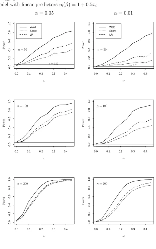
of score, Wald and LR tests in ZMGP regression models for samples of size n = 50,100,200. For brevity we report only some results from this study. A ZMGP model withϕ= 2,ωj = 0.05jforj= 0, . . . ,9 and linear predictorsηi(β) = 1 + 0.5xi
for i = 1, . . . , n and n = 50,100,200 was taken as a working model. As above, covariates xi’s were taken uniformly from (0,1). For each combination of sample
size and model we simulated 1000 sets of responses from the working model. This simulation setup implies that the probability of obtaining zero outcomes from the GP distribution with parameters ϕ = 2 and µi = exp(ηi(β)) varies between 0.11
and 0.25 for i = 1, . . . , n. For a better visualization we displayed our findings in Figure 1. The power of the tests between two neighbour knot points ωj and ωj+1 for j = 0, . . . ,8 is obtained by linear interpolation. From Figure 1 we see that all three tests maintain approximately their size, while the Wald test is much powerful than the LR test and even more powerful than the score test. A sample size of 50 is needed for the Wald test to achieve 80% power at ω = 0.40 and level α = 0.05 while for the score test a sample size of 100 is not sufficient. Taking the total cost for sampling and statistical inference the Wald test will be much more effective than the score test. The loss in power for the score test compared to the Wald test lies between 46% and 87% for sample size n = 50 and between 22% and 73% for sample size n=100. In contrast to the ZMP case, for the sample size n = 200 the percent difference in the power for the score and Wald tests is still significant and lies between 2% and 56%. Thus the score test performs worse when an additional overdispersion parameter compared to the Poisson distribution is allowed. Moreover the LR test has significantly higher power than the score test which was not the case in ZMP regression. The percent difference in power for the score and LR tests is between 8% and 64% forn= 50, 8% and 36% forn= 100, 1% and 20% forn= 200. With regard to the Wald and LR tests we observed that the LR test results in power loss up to 68% compared to the Wald test.
5.2
Apple propagation data
Ridout et al. (2001) analyzed data on the number of roots produced by 270 shoots of a certain apple cultivar. The shoots had been produced under an 8– or 16– hour photoperiod (Factor ”P”) in culture systems that utilized one of four different concentrations of cytokinin BAP (Factor ”H”) in the culture medium (for more details see Ridout and Dem´etrio (1992) and Marin et al. (1993)). Note that the data contain a large number of zero responses for the 16–hour photoperiod . Ridout et al. (2001) derived a score test for testing a zero-inflated Poisson regression model against zero-inflated negative binomial alternative and showed that zero-inflated Poisson model is unsuitable for these data.
Here we consider two different ZMGP models for the entire data and one ZMGP model for its part that have been collected under 16–hour photoperiod. In the first
Figure 1: Estimated upper tail probabilities for Wald, LR and score statistics at χ21,1−α in the ZMGP regression based on 1000 samples from the ZMGP model with linear predictors ηi(β) = 1 + 0.5xi
0.0 0.1 0.2 0.3 0.4 0.0 0.2 0.4 0.6 0.8 1.0 Wald Score LR 0.0 0.1 0.2 0.3 0.4 0.0 0.2 0.4 0.6 0.8 1.0 Wald Score LR 0.0 0.1 0.2 0.3 0.4 0.0 0.2 0.4 0.6 0.8 1.0 0.0 0.1 0.2 0.3 0.4 0.0 0.2 0.4 0.6 0.8 1.0 0.0 0.1 0.2 0.3 0.4 0.0 0.2 0.4 0.6 0.8 1.0 0.0 0.1 0.2 0.3 0.4 0.0 0.2 0.4 0.6 0.8 1.0 PSfrag replacements ω ω ω ω ω ω n= 50 n= 50 n= 100 n= 100 n= 200 n= 200 α= 0.05 α= 0.05 α= 0.01 α= 0.01 P ow er P ow er P ow er P ow er P ow er P ow er
model for the entire data (Model 1)µmay take different values only for two levels of Factor ”P”, while in the second model (Model 2)µmay take different values for each of the eight treatment combinations (”P∗H”). For the partial data we fit the ZMGP model analogously to Model 2, i.e. µ takes different values for each four levels of Factor ”H”. This model is further referred as Model 3. Overdispersion parameter ϕ
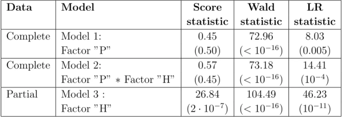
is taken to be constant in all models. Further we are interested in testing for zero-modification, i.e. the null hypothesis H0 :ω= 0 against the alternative H1 :ω6= 0. The values of the corresponding score, Wald and LR statistics for testing zero-modification are given in Table 2. Thus the Wald and LR tests clearly indicate that a simple GP regression without zero-modification is not sufficient for the whole apple propagation data as well as for its part with 16–hour photoperiod . The score test detects zero-modification only in the partial data and is not powerful enough to do it in the entire data. Moreover we see that for the partial data the Wald test gives much higher evidence for zero-modification than the LR and score tests which is due to the fact that the Wald test is much more powerful compared to them, as seen in the simulation.
For the partial data the ZMGP model and the the corresponding GP model are compared with respect to their fit to the empirical mean E(Y\|H=i) and variance
\
V ar(Y|H =i) (i= 1, . . .4) for the 4 different levels of Factor ”H”. Recall that the data contains replications for each level of Factor ”H”, therefore the E(Y\|H=i) and V ar(\Y|H =i) (i= 1, . . .4) can be computed. Further the mean and variance in the GP and ZMGP regression models are given by
E(Y|H =i) = exp xt iβ GP , V ar(Y|H =i) = (ϕGP )2exp xtiβGP
Table 2: The values of the score, Wald and LR statistics for testing zero-modification in the apple propagation data. The corresponding p–values are given in parenthesis.
Data Model Score Wald LR
statistic statistic statistic
Complete Model 1: 0.45 72.96 8.03 Factor ”P” (0.50) (<10−16) (0.005) Complete Model 2: 0.57 73.18 14.41 Factor ”P” ∗ Factor ”H” (0.45) (<10−16) (10−4) Partial Model 3 : 26.84 104.49 46.23 Factor ”H” (2·10−7) (<10−16) (10−11)
and E(Y|H =i) = (1−ω) exp xt iβ ZMGP , V ar(Y|H =i) = (1−ω) exp xtiβZMGP (ϕGP )2+ωexp xtiβZMGP , respectively. Here (ϕGP ,βGP ) and (ϕZMGP , ω,βZMGP
) denote the parameters of the GP and ZMGP models, respectively. Hence confidence intervals (CI) for the mean and variance of the both regressions can be constructed and plotted for all covariates xi (i = 1, . . . ,4) on the basis of the Delta method (van der Vaart (1998)) and asymptotic normality of the ML estimator ˆδ in ZMGP and GP regression models (Theorem 1 and Remark (ii)).
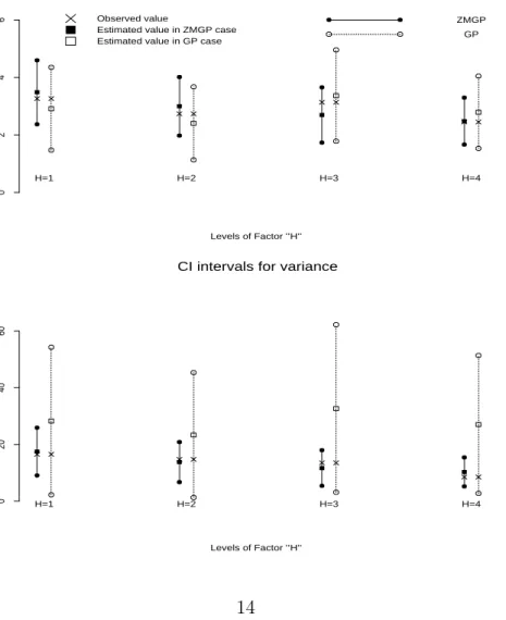
From Figure 2 we see that CI in the ZMGP case are always shorter and predicted values for mean and variance are more closer to their empirical values than in the GP
Figure 2: Confidence intervals (CI) for the mean (top panel) and variance (bottom panel) of the partial apple propagation data for ZMGP and GP models
CI intervals for mean
Levels of Factor ’’H’’ Range of CI H=1 H=2 H=3 H=4 0 2 4 6 Observed value
Estimated value in ZMGP case Estimated value in GP case
ZMGP GP
CI intervals for variance
Levels of Factor ’’H’’ Range of CI H=1 H=2 H=3 H=4 0 20 40 60
case. The only exception is the prediction of the mean in the case of Level 3 of Factor ”H” where the GP regression better estimates the mean. This is caused by the fact that frequency of observed zero responses is here lower compared to other levels of Factor ”H” (40% (H= 3) versus 50% (H = 1), 53.3% (H= 2) and 47.5% (H= 4)). The ML estimates and the corresponding asymptotic 95% confidence intervals for the zero-modification parameterω and overdispersion parameterϕgiven in Table 3 also support the necessity of zero-modification in GP models for the apple propagation data.
Table 3: ML estimators and the corresponding 95% confidence intervals (CI) forωand ϕ
in the ZMGP regression for the apple propagation data.
Data Model ωˆ ϕˆ CI for ω CI for ϕ
Complete Model 1 0.2225 1.2782 (0.1714,0.2735) (1.1423,1.4141) Complete Model 2 0.2231 1.2427 (0.1720,0.2742) (1.1118,1.3736) Partial Model 3 0.4638 1.4154 (0.3749,0.5527) (1.1327,1.6981)
Gupta et al. (2004) also analyzed these data within the framework of a zero-inflated regression model associated with a RGP distribution. Their score tests strongly indicate that a zero-inflated RGP regression is suitable for the apple prop-agation data.
6
Conclusions and Discussions
This paper shows that the ML estimators in ZMGP (GP, ZMP) regression models possess similar asymptotic properties as GLM regression models despite the fact that the ZMGP (GP, ZMP) distribution does not belong to the exponential family. General results of Fahrmeir and Kaufmann (1985) for noncanonical links in GLM have been adopted for this purpose. The simulation study exhibits that the power of the score test for testing zero-modification in ZMP regression can be up to 43% lower than the power of the corresponding Wald test. In the case of ZMGP regression this difference increases up to 87%. The effect of the poor performance of the score test in our simulation studies can be seen in the analysis of the entire apple propagation data. The score test does not detect any zero-modification despite the high proportion of zeros observed for one level of Factor ”P”. Note that zero-inflated count regression models are found to be appropriate for this data by Ridout et al. (2001) and Gupta et al. (2004). Therefore we conclude that score test for testing zero-modification in ZMP and ZMGP models can be highly misleading and the Wald and LR tests should be used instead.
The ZMGP regression model presented here can be generalized by allowing a regression formulation for the overdispersion parameter ϕand zero-modification pa-rameter ω. In this case nonnested testing situations with regard to the choice of covariates for the parameters µ, ϕ and ω will arise. A possible way to deal with this is to use the Vuong’s test (Vuong (1989)). It should be noted that regression models associated with the RGP distribution will belong to this general class of regression models. Asymptotic theory for this general regression model as well as its application are under current investigation by the authors.
It is often of interest to test whether the GP regression is more appropriate for count regression data than the Poisson regression. This is the subject of our future work. The null hypothesis is here ϕ = 1 versus the alternative ϕ > 1. Note that in this testing problem the true parameter ϕ lies on the boundary of a parameter space and therefore we have to deal with a delicate boundary problem (see e.g. Vu and Zhou (1997)).
Appendix
The Hessian matrix Hn(δ) in the ZIGP regression may be partitioned as
Hn(δ) = ∂ln(δ) ∂ββt ∂ln(δ) ∂βϕ ∂ln(δ) ∂βω ∂ln(δ) ∂ϕβt ∂ln(δ) ∂ϕϕ ∂ln(δ) ∂ϕω ∂ln(δ) ∂ωβt ∂ln(δ) ∂ωϕ ∂ln(δ) ∂ωω , (13) where ∂ln(δ) ∂ββt , ∂ln(δ) ∂βϕ , ∂ln(δ)
∂βω are matrices of dimension (p+ 1)×(p+ 1), (p+ 1)×1,
(p+ 1)×1, respectively, and ∂ln(δ)
∂ϕϕ ,
∂ln(δ)
∂ϕω ,
∂ln(δ)
∂ωω are scalars. Entries hrs(δ)’s of Hn(δ) can be straightforwardly computed. For instance entries of the matrix ∂l∂ββn(δt)
are given by hrs(δ) := ∂ln(δ) ∂βrβs (14) = − n X i=1 1l{yi=0}xirxis(1−ω)µi(β)fi(β, ϕ) × [1−µi(β)/ϕ]gi(δ) + (1−ω)fi(β, ϕ)µi(β)/ϕ ϕ[gi(δ)]2 − n X i=1 1l{yi>0}xirxisµi(β) 1 ϕ− yi(yi−1)(ϕ−1) [µi(β) + (ϕ−1)yi]2 forr, s= 0, . . . , p.
Now set Hn(δ) = −Hn(δ). It is well known (see for example Mardia et al. (1979), p.98) that under mild general regularity assumptions which are satisfied
here that the Fisher information matrixFn(δ) is equal to EδHn(δ). Thus entries of Fn(δ) can be straightforwardly computed and are given by
fr,s(δ) = fs,r(δ) = n X i=1 xirxis(1−ω)µi(β)fi(β, ϕ) × [1−µi(β)/ϕ]gi(δ) + (1ϕg −ω)fi(β, ϕ)µi(β)/ϕ i(δ) + n X i=1 (1−ω)xirxisµi(β) µi(β)−2ϕ+ 2ϕ2 ϕ2(µ i(β)−2 + 2ϕ) − 1 ϕfi(β, ϕ) forr, s= 0, . . . , p ; fp+1,r(δ) = fr,p+1(δ) = n X i=1 xir(1−ω)fi(β, ϕ)µi(β) × gi(δ) [µi(β)/ϕ−1]ϕ−2g(1−ω)fi(β, ϕ)µi(β)/ϕ i(δ) − n X i=1 (1−ω)xirµi(β) 2(ϕ−1) ϕ2(µ i(β)−2 + 2ϕ) − fi(β, ϕ) ϕ2 forr = 0, . . . , p ; fp+2,r(δ) = fr,p+2(δ) =− n X i=1 xirfi(β, ϕ)µi(β) ϕgi(δ) forr = 0, . . . , p ; fp+1,p+1(δ) = − n X i=1 (1−ω)fi(β, ϕ)µi(β) ×gi(δ) (µi(β)−2ϕ)ϕ4−g(1−ω)fi(β, ϕ)µi(β) i(δ) + n X i=1 2(1−ω)µi(β) 1 ϕ2(µ i(β)−2 + 2ϕ) − fi(β, ϕ) ϕ3 ; fp+2,p+1(δ) = fp+1,p+2(δ) = n X i=1 fi(β, ϕ)µi(β) ϕ2g i(δ) and fp+2,p+2(δ) = n X i=1 [1−fi(β, ϕ)]2 gi(δ) +1−fi(β, ϕ) 1−ω ! .
The proof of Theorem 1 follows the proof of Theorem 4 given in Fahrmeir and Kaufmann (1985). In particular, we have to prove asymptotic normality of the normalized score vectors Ft/n2sn (Lemma 3) and show (Lemma 4) that
max
δ∈Nn(ε)k
where Vn(δ) :=F−n1/2Hn(δ)F−nt/2 for n= 1,2, . . .. The complex expression for the entries of the Fisher information matrix and Hessian matrix, respectively, requires more effort for proving Lemma 4 than in the case of the GLM.
First we proceed with two preliminary lemmas. Recall that we drop the depen-dency on δ0,β0, ϕ0 and use µi, Fn, E, etc.
Lemma 1. Let Y˜i ∼GP(µi, ϕ0) for i= 1, . . . , n be a sequence of random variables.
Then under assumptions (A2) and (A3), max i=1,...,nE 1 (µi+ (ϕ0−1) ˜Yi)k ≤C1 and max i=1,...,nE( ˜Y k i )≤C2
for any finite integer k >0, where C1 and C2 are positive constants depending only on k and δ0 .
Proof. Let us show the first inequality of the Lemma. It is evident using (A3) that
E 1 (µi+ (ϕ0−1) ˜Yi)k ≤ 1 µk i . (15) Now it follows max i=1,...,n 1 µk i = max i=1,...,n 1 exp (kxt iβ0) ≤ max x∈Kx 1 exp (kxtβ 0) ≤ C1(β0, k), since Kx is a compact and exp kxtβ0
is a continuous function of x. It should be noted thatC1(β0, k) is continuous with respect toβ0and well defined for allβ0 ∈B. Now we show the second inequality of the lemma. First, we reparametrize the GP distribution by introducing new parameters θi:=µi/ϕ0 and λ0:= (ϕ0−1)/ϕ0, i = 1, . . . , n. Consul and Shenton (1974) gave the following recurrence formula for the noncentral moments of the GP(θi, λ0) distribution:
(1−λ0)mi,k+1=θimi,k+θi ∂mi,k ∂θi +λ0 ∂mi,k ∂λ0 , k = 0,1,2, . . . , where mi,k:=E( ˜Yik).
Solving this recursion for fixed k shows that mi,k is a polynomial inθi, λ0 and 1/(1−λ0). Thus, mi,k is a continuous function with respect to (θi, λ0) and conse-quently, it is also continuous with respect to (µi, ϕ0). It follows now that
max i=1,...,nE( ˜Y k i ) = i=1max,...,nmi,k(θi, λ0) = max i=1,...,nmi,k(µi/ϕ0,(ϕ0−1)/ϕ0) ≤ max x∈Kx mk extβ0 /ϕ0,(ϕ0−1)/ϕ0 ≤ C2(δ0),
where mk := E( ˜Yk) and ˜Y ∼ GP(exp(xtβ0), ϕ0). It is not difficult to see that C2(δ0) is continuous with respect toδ0 and well defined for all δ0 ∈Kδ.
Lemma 2. Let Qk(y) be a polynomial of a finite order k (k ∈N) whose coefficients
are positive continuous functions of x,δandδ0. Further, letYi∼ZIGP(exp(xt
iβ0), ϕ0, ω0) for i= 1, . . . , n. If (A1)–(A3) hold then
max δ∈Nn(ε) max i=1,...,nE 1l{Yi>0}Qk(Yi) < C, where C is a positive constant depending on k and δ0.
Proof. Note that under (A1) the neighborhood Nn(ε) is a compact for any n ∈ N
and shrinks to δ0 for any ε >0 as n → ∞. Using Lemma 1 and the continuity of the coefficients of Qk, it follows now that
max δ∈Nn(ε) max i=1,...,nE 1l{Yi>0}Qk(Yi) ≤ max δ∈Nn(ε) max i=1,...,n(1−ω0)E Qk( ˜Yi) ≤ max δ∈N1(ε)xmax∈Kx (1−ω0)E Qk( ˜Y) ≤ C,
where ˜Yi ∼GP(exp(xtiβ0), ϕ0) and ˜Y ∼GP(exp(xtβ0), ϕ0).
Lemma 3. Under assumptions (A1)–(A3), F−n1/2sn ⇒D Np+3(0,Ip+3) as n → ∞, where Np+3(0,Ip+3) is a (p+ 3)-dimensional normal distribution with mean vector 0 and covariance matrix Ip+3.
Proof. According to the Cramer-Wald device, it is sufficient to show that a linear combination atF−n1/2sn converges in distribution to N(0,ata) for any vector a ∈
Rp+3 (a6=0). Without loss of generality, we setkak= 1.
Now observe that sn can be written as a sum of independent random vectors, namely sn=Pn
i=1sni, where sni= (s0,i, . . . , sp,i, sp+1,i, sp+2,i)t withsk,i:= sk,i(δ0) defined in (9), (10) and (11) for k = 0, . . . , p+ 2 andi= 1, . . . , n, respectively. Fur-ther, define independent random variablesξinbyξin :=atFn−1/2sni. SinceE(ξin) = 0
and V ar(Pn
i=1ξin) = 1, it is enough to show that the Lyapunov condition is
satis-fied, i.e. Ls:= n X i=1 E|ξin|s n−→→∞0, for some s >2,
say s = 3 (see for example Hoffmann-Jørgensen (1994), p. 393). Noticing that
kF−n1/2k2 = 1/λmin(Fn), it follows from (A1) that L3 ≤ n X i=1 E at 3 F −1/2 n 3 ksnik3 ≤ C n3/2 n X i=1 Eksnik3 ≤ √C n i=1max,...,nEk snik3.
Using an extension of the cr-inequality given by E m X i=1 ζi k ≤mk−1 m X i=1 E|ζi|k ( k >1, k ∈R), (16)
to m arbitrary random variablesζ1, . . . , ζm ( see, for example, Petrov (1995), p.58)
yields that
Eksnik3≤CE|s0,i|3+. . .+E|sp,i|3+E|sp+1,i|3+E|sp+2,i|3.
Thus, it remains to establish that maxi=1,...,nE|sr,i|3 is uniformly bounded in n
for r = 0, . . . , p+ 2. This will be shown for case r = 0, . . . , p. The remaining cases can be treated similarly. Without loss of generality, set r =p. Using now (16) with
m= 2, we have max i=1,...,nE|sp,i| 3 ≤ 22 max i=1,...,nE xip1l{yi=0} (1−ω0)fiµi ϕ0gi 3 + 22 max i=1,...,nE xip1l{yi>0} 1 + µi(yi−1) µi+ (ϕ0−1)yi − µi ϕ0 3! =: 4Ap(δ0) + 4Bp(δ0). The last step in the proof is now to show that
Ap(δ0)< C1 and Bp(δ0)< C3, (17) where C1 and C3 are some constants depending on δ0.
For proving (17) we note that
Ap(δ0)≤ max x∈Kxk xk3 (1−ω0)fiµi ϕ0gi 3 gi≤C1.
Let us now consider Bp(δ0). Simple arguments with Inequality (16), Cauchy-Schwarz inequality and Lemma 1, respectively, give
Bp(δ0) ≤ max i=1,...,nE (1−ω0)|xir|3· 1 + µi( ˜Yi−1) µi+ (ϕ0−1) ˜Yi − µi ϕ0 3 ≤ Cmax x∈Kx (1−ω0)kxk3 13+E µi( ˜Y −1) µi+ (ϕ0−1) ˜Y 3 + µi ϕ0 3 ≤ C1(δ0) +C2(δ0) max x∈Kx E Y˜ −1 3 ≤ C1(δ0) +C2(δ0) max x∈Kx r EY˜ −16 ≤ C3(δ0),
where ˜Yi ∼GP (µi, ϕ0) for i= 1, . . . , n and ˜Y ∼GP exp(xtβ0), ϕ0
Lemma 4. Under the assumptions (A1)–(A3),
max
δ∈Nn(ε)k
Vn(δ)−Ip+3k−→P 0 for all >0. (18) Proof. It holds a.s. that
kVn(δ)−Ip+3k = F −1/2 n [Hn(δ)−Fn]F−nt/2 ≤ λ 1 min(Fn)k Hn(δ)−Fnk ≤ Cn kHn(δ)−Fnk ≤ C 1 n(Hn(δ)−EHn(δ)) +C 1 n(EHn(δ)−Fn) . Thus, conditions max δ∈Nn(ε) 1 n(Hn(δ)−EHn(δ)) P −→0 (19) and max δ∈Nn(ε) 1 n(EHn(δ)−Fn) −→ 0 (20) imply (18).
In order to show (19) it is enough to establish that the maximum overδ∈Nn(ε)
of the absolute value of the (r, s)-element of the random matrix [Hn(δ)−EHn(δ)]/n converges to zero in probability, i.e.
max δ∈Nn(ε) |hrs(δ)−Ehrs(δ)| n P −→0.
Note that the Hessian matrix given in (13) has 6 different types of entries. We shall illustrate the above convergence for hrs(δ)’s defined in (14). The remaining cases
can be treated similarly. Without loss of generality, we show max δ∈Nn(ε) 1 n(hp,p(δ)−Ehp,p(δ)) P −→0. (21) LetZi := 1l{Yi>0}Yi(Yi−1),Ui(β, ϕ) :=µi(β) + (ϕ−1)Yi, qi,p(δ) :=x 2 ipµi(β)(ϕ−1) and vi,p(δ) :=x2ip(1−ω)fi(β, ϕ)µi(β) [1−µi(β)/ϕ]gi(δ) + (1−ω)fi(β, ϕ)µi(β)/ϕ ϕ[gi(δ)]2
for i= 1, . . . , n. It easy to see that (21) will now follow from the next three condi-tions: max δ∈Nn(ε) 1 n n X i=1 vi,p(δ) 1l{Yi=0}−E(1l{Yi=0}) P −→0, max δ∈Nn(ε) 1 n n X i=1 qi,p(δ) ϕ 1l{Yi>0}−E(1l{Yi>0}) P −→0 max δ∈Nn(ε) 1 n n X i=1 qi,p(δ) Zi [Ui(β, ϕ)]2 − E Zi [Ui(β, ϕ)]2 P −→0. (22) Since they have a similar structure we only establish the validity of the last relation. It is worth to recall that the dependency on δ0, β0 and ϕ0 is always dropped.
Observe that the right hand side of (22) may be bounded by a sum of
An = max δ∈Nn(ε) 1 n n X i=1 qi,p(δ) Zi [Ui(β, ϕ)]2 − Zi U2 i , Bn = max δ∈Nn(ε) 1 n n X i=1 qi,p(δ) E Zi [Ui(β, ϕ)]2 − E Zi U2 i , Dn = max δ∈Nn(ε) 1 n n X i=1 qi,p(δ) Zi U2 i −E Zi U2 i .
For An we have the following bounds a.s.:
An ≤ max δ∈Nn(ε) 1 n n X i=1 |qi,p(δ)Zi| µ2 i(β)µ2i · |Ui(β, ϕ) +Ui| |µi(β)−µi+ (ϕ−ϕ0)Yi| ≤ max δ∈Nn(ε) 1 n n X i=1 |qi,p(δ)Zi| µ2 i(β)µ2i · |(Yi+ 1)(µi(β) +µi+ϕ+ϕ0−2)| × |µi(β)−µi+ (ϕ−ϕ0)Yi| ≤ Cn1 n X i=1 Zi(Yi+ 1) ! max δ∈Nn(ε) max x∈Kx exp(xtβ)−exp(xtβ0) + C1 n n X i=1 ZiYi(Yi+ 1) ! max δ∈Nn(ε)| ϕ−ϕ0| =: ABn+ACn. (23)
It is not difficult to see that
1 n n X i=1 Zi(Yi+ 1) converges in probability as n→ ∞to lim n→∞ 1 n n X i=1 E(Zi(Yi+ 1))
which is finite by Lemma 2.
These facts and the continuity inβof the function maxx∈Kx
exp(xtβ)−exp(xtβ0)
with value zero at β =β0 yield that ABn converges to 0 in probability asn→ ∞.
Convergence of ACn to 0 in probability may be proven in the same way.
Using similar arguments as above one can show thatBnconverges to 0. To prove
Dn → 0 in probability, observe that the function maxi=1,...,n|qi,p(δ)−qi,p(δ0)| can be bounded from above by the following continuous function of δ
Cmax x∈Kx exp(xtβ)(ϕ−1)−exp(xtβ0)(ϕ0−1)
with zero at δ =δ0. The desired result now follows from the law of large numbers and standard arguments.
It remains to show (20). We will show max δ∈Nn(ε) [EHn(δ)−Fn] rs n → 0 (24)
and again restrict our proof to the case r=s=p. It easy to see that condition (24) will follow from the next three conditions :
max δ∈Nn(ε) 1 n n X i=1 (vi,p(δ)−vi,p)E(1l{Yi=0}) →0, (25) max δ∈Nn(ε) 1 n n X i=1 qi,p(δ) ϕ − qi,p ϕ0 E(1l{Yi>0}) →0, (26) max δ∈Nn(ε) 1 n n X i=1 qi,p(δ)E Zi [Ui(β, ϕ)]2 −qi,pE Zi Ui2 →0. (27) Now we see that the same technique used for deriving (22) can be employed to establish the convergence results (25)–(27).
Acknowledgement
Both authors gratefully acknowledge the support of the Deutsche Forschungsge-meinschaft (Cz 86/1-1). They also thank Marie Huˇskov´a and Axel Munk for helpful discussions.
References
Bae, S., F. Famoye, J. T. Wulu, A. A. Bartolucci, and K. P. Singh (2005). A rich family of generalized Poisson regression models.Math. Comput. Simula-tion 69(1-2), 4–11.
Consul, P. C. (1989). Generalized Poisson distributions, Volume 99 of Statistics: Textbooks and Monographs. New York: Marcel Dekker Inc. Properties and applications.
Consul, P. C. and F. Famoye (1992). Generalized Poisson regression model. Comm. Statist. Theory Methods 21(1), 89–109.
Consul, P. C. and G. C. Jain (1970). On the generalization of Poisson distribution. Ann. Math. Statist. 41, 1387.
Consul, P. C. and L. R. Shenton (1974). On the probabilistic structure and proper-ties of discrete Lagrangian distribution. In G. Patil, S. Kotz, and J. Ord (Eds.), A modern course on statitical distributions in scientific work, Volume 1, pp. 41–57. D.Reidel Publishing Company, Boston.
Consul, P. C. and M. M. Shoukri (1985). The generalized Poisson distribution when the sample mean is larger than the sample variance. Comm. Statist. Simulation Comput. 14(3), 667–681.
Czado, C. and I. Sikora (2002). Quantifying overdispersion effects in count regression data. Discussion paper 289 of SFB 386 ( http://www.stat.uni-muenchen.de/sfb386/).
Dietz, E. and D. B¨ohning (2000). On estimation of the Poisson parameter in zero-modified Poisson models.Comput. Statist. Data Anal. 34(4), 441–459. Fahrmeir, L. and H. Kaufmann (1985). Consistency and asymptotic
normal-ity of the maximum likelihood estimator in generalized linear models. Ann. Statist. 13(1), 342–368.
Famoye, F. (1993). Restricted generalized Poisson regression model. Comm. Statist. Theory Methods 22(5), 1335–1354.
Famoye, F. and K. P. Singh (2003). On inflated generalized Poisson regression models.Adv. Appl. Stat. 3(2), 145–158.
Famoye, F. and K. P. Singh (2006). Zero-inflated generalized Poisson model with an application to domestic violence data. Journal of Data Science 4(1), 117– 130.
Gschl¨oßl, S. and C. Czado (2005). Modelling count data with overdispersion and spatial effects. Discussion paper 412 of SFB 386 ( http://www.stat.uni-muenchen.de/sfb386/).
Gupta, P. L., R. C. Gupta, and R. C. Tripathi (2004). Score test for zero inflated generalized Poisson regression model.Comm. Statist. Theory Methods 33(1), 47–64.
Hall, D. B. and K. S. Berenhaut (2002). Score tests for heterogeneity and overdis-persion in zero-inflated Poisson and binomial regression models. Canad. J. Statist. 30(3), 415–430.
Hoffmann-Jørgensen, J. (1994). Probability with a view toward statistics. Vol. I. Chapman & Hall Probability Series. New York: Chapman & Hall.
Jansakul, N. and J. P. Hinde (2002). Score tests for zero-inflated Poisson models. Comput. Statist. Data Anal. 40(1), 75–96.
Joe, H. and R. Zhu (2005). Generalized Poisson distribution: the property of mixture of Poisson and comparison with negative binomial distribution.Biom. J. 47(2), 219–229.
Lambert, D. (1992). Zero-inflated poisson regression, with an application to de-fects in manufacturing.Technometrics 34(1), 1–14.
Lawless, J. F. (1987). Negative binomial and mixed Poisson regression.Canad. J. Statist. 15(3), 209–225.
Mardia, K. V., J. T. Kent, and J. M. Bibby (1979). Multivariate analysis. Lon-don: Academic Press [Harcourt Brace Jovanovich Publishers]. Probability and Mathematical Statistics: A Series of Monographs and Textbooks.
Marin, J., O. Jones, and W. Hadlow (1993). Micropropagetion of columnar apple trees.Journal of Horticultiral Science 68, 289–297.
Mullahy, J. (1986). Specification and testing of some modified count data models. J. Econometrics 33(3), 341–365.
Petrov, V. V. (1995).Limit theorems of probability theory sequences of independent variables. Oxford studeis in probability. Oxford: Clarendon Press.
Ridout, M. and C. G. B. Dem´etrio (1992). Generalized linear models for positive count data.Revista de Matematica e Estatistica 10, 139–148.
Ridout, M., J. Hinde, and C. G. B. Dem´etrio (2001). A score test for testing a zero-inflated Poisson regression model against zero-inflated negative binomial alternatives.Biometrics 57(1), 219–223.
Stewart, G. W. (1998). Matrix algorithms. Vol. I. Philadelphia, PA: Society for Industrial and Applied Mathematics. Basic decompositions.
van den Broek, J. (1995). A score test for zero inflation in a Poisson distribution. Biometrics 51(2), 738–743.
van der Vaart, A. W. (1998).Asymptotic statistics. Cambridge Series in Statistical and Probabilistic Mathematics. Cambridge: Cambridge University Press. Verbeke, G. and G. Molenberghs (2003). The use of score tests for inference on
variance components.Biometrics 59(2), 254–262.
Vu, H. T. V. and S. Zhou (1997). Generalization of likelihood ratio tests under nonstandard conditions.Ann. Statist. 25(2), 897–916.
Vuong, Q. H. (1989). Likelihood ratio tests for model selection and nonnested hypotheses.Econometrica 57(2), 307–333.