NBER WORKING PAPER SERIES
IS THERE AN OPTIMAL INDUSTRY FINANCIAL STRUCTURE?
Peter MacKay Gordon M. Phillips
Working Paper9032
http://www.nber.org/papers/w9032
NATIONAL BUREAU OF ECONOMIC RESEARCH 1050 Massachusetts Avenue
Cambridge, MA 02138 July 2002
MacKay is from the Edwin L. Cox School of Business, Southern Methodist University and Phillips is from the Robert H. Smith School of Business, University of Maryland and is a visiting professor at MIT Sloan School of Management. We wish to thank Murray Frank, Gerald Garvey, Mike Long, Robert McDonald, Vojislav Maksimovic, Nagpurnanand Prabhala, Alexander Reisz, Toni Whited, and seminar participants at the 2002 American Finance Association, the Atlanta Finance Consortium, the 2001 Rutgers Conference on Capital Structure, Southern Methodist University, the University of Kentucky, and the University of British Columbia for helpful comments. MacKay can be reached by email at [email protected], homepage: http://faculty.cox.smu.edu/pmackay.html. Phillips can be reached by email at
[email protected], homepage: www.rhsmith.umd.edu/Finance/gphillips/. The authors alone are
responsible for the work and any errors or omissions. The views expressed herein are those of the authors and not necessarily those of the National Bureau of Economic Research.
© 2002 by Peter MacKay and Gordon M. Phillips. All rights reserved. Short sections of text, not to exceed two paragraphs, may be quoted without explicit permission provided that full credit, including © notice, is given to the source.
Is There an Optimal Industry Financial Structure? Peter MacKay and Gordon M. Phillips
NBER Working Paper No. 9032 July 2002
JEL No. G3
ABSTRACT
We examine how intra-industry variation in financial structure relates to industry factors and whether real and financial decisions are jointly determined within competitive industries. We find that industry and group factors beyond standard industry fixed effects are also important to firm financial structure. Firm financial leverage, capital intensity, and cash-flow risk are interdependent decisions that depend on the firm’s proximity to the median industry capital-labor ratio, the actions of firms within its industry quintile, and its status as entrant, incumbent, or exiting firm. Our results support competitive industry equilibrium models of financial structure in which debt, technology, and risk are simultaneous decisions.
Peter MacKay Gordon M. Phillips
Edwin L. Cox School of Business R.H. Smith School of Management Southern Methodist University University of Maryland
Dallas, TX 75275-0333 College Park, MD 20742
[email protected] and NBER
Despite extensive financial structure research since Myers (1984) and Harris and Raviv (1991), important puzzles remain.1 The importance of industry to firm financial structure and the
simultaneity of financial and real-side decisions are two such related puzzles. Although it is widely held that industry factors are important to firm financial structure, empirical evidence shows that there is wide variation in financial structure even after controlling for industries.2 Researchers
routinely remove industry fixed effects by including dummy variables or sweeping out industry means and use the remaining variation to test how firm characteristics affect financial policy. Yet, this approach does not tell us how industry affects firm financial structure, nor why financial structure and real-side characteristics vary so widely across firms within a given industry. Recent theoretical models (Dammon and Senbet, 1988, Leland, 1998) stress the simultaneity of real and financial decisions – yet little is known about the empirical relevance of the simultaneity of these decisions. We thus examine these two unresolved but related questions: How important are industry factors to firm financial structure? Can industry equilibrium forces explain how firms distribute within industries – both along real-side and financial dimensions?
We address these questions by directly examining how intra-industry variation in financial structure relates to industry factors and whether real and financial decisions are jointly determined within competitive industries.3 We provide broad evidence of how industry affects firm financial
structure, and test predictions of competitive-industry equilibrium models (Maksimovic and Zechner, 1991, Williams, 1995, and Fries, Miller, and Perraudin, 1997). Similar to Miller’s (1977) irrelevance result, these studies illustrate how conclusions reached in a partial-equilibrium framework are fundamentally altered, even reversed, as the equilibrium setting is aggregated to the level of an industry or the economy. In so doing, we go beyond tests of static trade-off and pecking-order
1 Recent empirical papers on financial structure examine static trade-off and pecking-order theories (Fama and French, 2002, Frank and Goyal, 2002), taxes (Graham, 2000), risk shifting (Parrino and Weisbach, 1999), and technology (MacKay, 2002). Bertrand and Schoar (2001) find that manager fixed effects are important to financial structure. Their results are related to ours in that firms deviate from industry “norms” on multiple dimensions. 2 An early study that documents wide intra-industry variation in financial structure is Remmers, Stonehill, Wright,
and Beekhussen (1974). Chaplinsky (1983) shows that industry dummies explain a small share of the variation in financial structure. Bradley, Jarrell, and Kim (1984) find that industry is important, but once regulated industries are excluded, industry dummy variables add only 10.1 percent additional explanatory power to the 23.6 percent variation in financial structure explained by firm volatility, non-debt tax shields, and advertising and R&D. 3 Chevalier (1995), Phillips (1995) and Kovenock and Phillips (1997) show that firms take into account other firms’
financial and real decisions in imperfectly competitive industries. Opler and Titman (1994) show that highly leveraged firms lose market share in concentrated industries after negative industry shocks.
2
theories and examine whether the real and financial decisions of individual firms are related to decisions of industry peers.
We investigate the impact of simultaneity, both as a practical empirical matter and as a test of recent theory, by estimating single- and simultaneous-equation regressions for financial leverage, capital-labor ratios, and cash-flow volatility. We test predictions of industry equilibrium models by including measures of a firm’s position within its industry, such as the similarity of its capital-labor ratio to the industry median capital-labor ratio, the actions of firms inside and outside the firm’s industry-year quintile, and its status as an entrant, incumbent, or exiting firm.
We precede these specific tests of industry equilibrium model predictions with a broader investigation of inter- and intra-industry variation in financial structure. We document extensive cross-sectional variation in financial leverage within 142 competitively-structured U.S. industries between 1981 and 2000. A simple analysis of variance shows that most of the variation in financial structure arises within industries rather than between industries. Two-, three-, and four-digit SIC industry fixed effects combined account for only 11% of variation in financial structure (7% by two-digit SIC). In contrast, firm fixed effects explain 64% of variation in financial structure, and the remaining 25% is within-firm variation.
Given the relative unimportance of industry fixed effects in explaining financial structure, we examine whether other industry factors can account for some of the wide variation observed within
industries. Following industry equilibrium models, we do so by testing the interactions between debt, technology, and risk, and whether a firm’s industry position affects how it chooses these variables.
Consistent with Maksimovic and Zechner (1991), we find that firms that deviate from the industry median technology use more financial leverage than firms operating technologies near the industry median, and that changes in financial leverage are positively related to changes in risk. We also find that changes to a firm’s financial leverage are positively related to changes in financial leverage made by other firms within its financial-leverage industry quintile, but not to changes by firms outside its industry quintile. Similar patterns obtain for capital intensity and risk. These results
3
suggest that even in competitively-structured industries: 1) firms form cohorts within their industry, and, 2) strategic complementarities arise along real and financial dimensions within these cohorts.
To investigate the dynamic aspects of the industry equilibria developed by Williams (1995) and Fries et al. (1997), we present transition frequencies for firms entering, staying, or leaving their industries. Comparing industry quintiles for the first and second periods (1981-1990 and 1990-2000), we find that for all the variables we consider (financial leverage, capital-labor ratios, cash-flow volatility, profitability, and asset size), persistence rates for incumbent firms are well above what would be expected if firms were uniformly randomly redistributed across quintiles in the second period. This suggests that that even in competitively-structured industries, firm characteristics evolve slowly, and that firms retain their industry rankings, consistent with the intra-industry diversity predicted by industry equilibrium theories.
Williams (1995) predicts that because of dissipative perks and differential access to capital, the equilibrium structure of industries is characterized by a core of large, stable, profitable, capital-intensive, financially-leveraged firms and a competitive fringe of small, risky, non-profitable, labor-intensive firms. We find support for this prediction for entrant firms and partial support for exiting firms, although perhaps not surprisingly, exiting firms carry more debt than incumbents or entrants.
We find that new entrants and incumbents that switch industries operate at the fringe of their industries, being smaller, riskier, less profitable, and more labor-intensive than core incumbent firms. However, we find only weak support for Williams’ prediction that entrants carry less debt than incumbents. In addition, firms that leave their industries are much more indebted than entrants or incumbents, suggesting that financial distress causes some fringe firms to deviate from the Williams’ equilibrium prototype and exit with high financial leverage and capital-labor ratios.
We make two major contributions in this paper. First, we provide evidence on the importance of within-industry equilibrium forces. We find that industry and group factors beyond standard industry fixed effects are also important to firm financial structure. Limited industry-mean reversion occurs as firms mostly remain in their industry groups – both on real and financial dimensions.
4
Consistent with industry equilibrium models, we find that proxies for a firm’s position within its industry add statistical and economic significance in explaining a firm’s real and financial decisions.
Second, we identify and account for the interactions between financial structure, technology, and risk choice. We find that accounting for the simultaneity of these decisions is important economically – not just econometrically. Accounting for this simultaneity impacts multiple relations, including the relations between financial structure and risk, and between risk and profitability.
Overall, our paper bridges the gap between empirical studies of partial-equilibrium models, which simply use firm variation to test representative-firm behavior, and industry equilibrium models, which endogenize firm variation and link firm-level decisions to broader equilibrium forces. The remainder of the paper is organized as follows. Section II reviews the financial-structure literature and develops empirical hypotheses from the industry equilibrium models. Section III describes our data sources, sample selection, and the variables we use to test these hypotheses. Section IV discusses our univariate and multivariate results. Section V concludes.
II. The Importance of Industry to Financial Structure
Most financial-structure research is partial-equilibrium, relating firm financial policy to agency conflicts and capital-market imperfections. This approach has produced important contributions, including static trade-off and pecking-order theories, and fueled a large body of empirical research, including recent work by Fama and French (2002) and Frank and Goyal (2002).
We focus on the importance of industry equilibrium forces to firm financial structure.4 The
literature most relevant for our analysis is a recent theoretical body of research that emphasizes industry equilibrium forces in the spirit of Miller (1977). These industry equilibrium models focus on how real and financial decisions are jointly determined within competitive industries (Maksimovic and Zechner, 1991, Williams, 1995, and Fries et al., 1997). The industry equilibrium approach offers additional insights, namely, that firms make their individual real and financial decisions in reference
4 A recent paper by Almazan and Molina (2001) contrasts multiple explanations for the dispersion in financial structure within industries. They focus only on the largest firms in each industry and include both competitive and imperfectly-competitive industries.
5
to the collective decisions of their industry peers, and that equilibrium outcomes imply intra-industry diversity rather than industry-wide targets.5
Before we test specific models of the industry equilibrium literature, we first explore the relevance of industry to real-side and financial interactions by providing broad evidence on the importance of industry to financial structure, technology, and risk choice. Using simple non-parametric and non-parametric methods, we examine the variation within and between industries in financial structure as well as technology, risk, profitability, and firm size. This analysis gives a detailed picture of how these key variables vary, with each other and nonlinearly, within an industry. Finally, we estimate simultaneous-equation regressions that test whether, as predicted by industry-equilibrium theory, a firm’s position within its industry interacts with its real and financial decisions. The remainder of this section reviews the industry equilibrium models and describes how we test their empirical predictions. Maksimovic and Zechner (1991), Williams (1995), and Fries et al. (1997) show that industries can play a subtle role in the determination of within-industry financial structure. Put simply, these models emphasize the simultaneity of financial structure, technology, and risk, and endogenize the distribution of firm characteristics within industries. Thus, perhaps more so than for tests of partial-equilibrium theories, our tests must address the simultaneity of these real- and financial-decision variables, and the endogeneity of firm characteristics relative to industry peers.
Maksimovic and Zechner (1991) assume that firms can choose between a “safe” technology with a certain marginal cost, and a “risky” technology with an uncertain cost. In partial equilibrium, no debt is issued since shareholders would expropriate bondholders by picking the risky technology. However, each firm has an incentive to finance with debt and adopt the risky technology because by raising (lowering) output in good (bad) states, the risky technology initially has greater expected profits and risk than the safe technology. As more firms pick the risky technology, the price of output more closely tracks that technology’s marginal cost; the risky technology becomes less risky and less profitable. Equilibrium obtains when the expected value of the ex-ante safe and risky technologies is
5 The jointness of real and financial decisions is also central to a number of partial-equilibrium models such as Dammon and Senbet (1988), Mauer and Triantis (1994), and Leland (1998). However, the empirical evidence is limited. MacKay (2002) does find significant interactions between real-side flexibility and financial structure.
6
equal and firms are indifferent between high-debt, high-risk and low-debt, low-risk configurations. Thus, what Maksimovic and Zechner (1991) show is that in industry equilibrium, firm financial structure is irrelevant because a technology’s risk and profitability depend not only on ex-ante
characteristics but also on how many firms adopt that technology.
We test the following three empirical predictions from Maksimovic and Zechner (1991). First, as firms depart from the main industry technology they will also use more debt in their financial structure. Second, because the equilibrium is characterized by high-debt, high-risk and low-debt, low-risk configurations, we should observe a positive relation between financial leverage and cash-flow volatility (our risk proxy). Third, because a firm’s risk and profitability depend on the technology decisions of all firms in the industry, we should observe an inverse relation between cash-flow volatility and a firm’s proximity to the median technology (which we term the “natural hedge”), and between profitability and the firm’s proximity to the median industry technology. An important feature of Maksimovic and Zechner’s model is that debt, technology, and risk are chosen endogenously and simultaneously, a fact that our empirical approach must support.
Williams (1995) extends Maksimovic and Zechner’s (1991) model by endogenizing entry and exit and adding exogenous perks consumption. Williams assumes that firms produce a homogeneous good using either a high variable-cost, labor-intensive technology with no capital outlay, or a low variable-cost, capital-intensive technology requiring capital-market financing. Because managers cannot credibly commit to forego their perks, capital is rationed in equilibrium even though the capital market is perfectly competitive. Even as the cost of entry converges to zero, a core of capital-intensive firms earns positive profits because this agency problem prevents the fringe of labor-intensive firms from raising capital and dissipating the core firms’ monopoly rents.
Like Maksimovic and Zechner (1991), Williams (1995) characterizes the industry equilibrium distribution of debt and firm characteristics, and explains firm heterogeneity within industries. By allowing for entry, Williams predicts an asymmetric equilibrium industry structure characterized by a core of large, stable, profitable, capital-intensive, financially-leveraged firms flanked by a competitive fringe of small, risky, non-profitable, labor-intensive firms.
7
We use several empirical strategies to test the Williams (1995) equilibrium industry structure. First, we report differences between industry-year adjusted means for incumbents and firms that enter or exit their industries (Table II). Second, we produce separate analyses of variance of industry and firm effects for incumbents and firms that enter or exit their industries (Table III). Third, we use transition frequencies to test Williams’ prediction that core (fringe) firms belong to the center (tails) of the industry distribution for financial leverage, capital intensity, risk, profitability, and size (Table VI). Finally, we include dummies for entry and exit in our multivariate regressions (Table IX).
Fries et al. (1997) use a contingent-claims approach to analyze optimal financial structure in a competitive-industry equilibrium that combines features of the previous models. Like Williams (1995), they allow for endogenous firm entry and exit. Like Maksimovic and Zechner (1991), they incorporate shareholder-bondholder conflicts and corporate debt tax-shields. Fries et al. (1997) find that as a result of a trade-off between tax advantages and agency costs, a firm optimally adjusts its financial leverage upward after inception. To test this prediction, we test for differences in financial leverage between the year of entry and the years following entry. We also test for differences in financial leverage between the year of exit and the years preceding exit.
We capitalize on certain similarities between the industry equilibrium models. For instance, by focusing on capital-labor ratios as a measure of technology, we directly incorporate a feature of the Williams (1995) model, where firms are either capital-intensive or labor-intensive. We also use capital-labor ratios to implement Maksimovic and Zechner’s (1991) natural hedge concept, where firms that depart from the median industry capital-labor ratio experience greater cash-flow volatility.
On a broader level, our major contribution is in examining the central common theme of these models – that firms’ debt, technology, and risk decisions are jointly determined – not in testing one model against the others. It is important to note that we are not conducting structural tests of these models but rather are testing certain predictions that arise out of their industry assumptions and the central theme that real and financial decisions are simultaneously determined as result of industry equilibrium forces.
8
To examine this central theme, we estimate simultaneous-equation regression models for financial leverage, capital-labor ratios, and cash-flow volatility. Empirically, as well as theoretically, we allow the financial structure decision to depend on risk and technology choice and vice versa. We account for interactions between these dependent variables by including each of the remaining two variables as regressors for the dependent variables featured in each equation. We use Generalized Method of Moments (GMM) to reflect the correlation of the residuals across these equations and to instrument endogenous right-hand-side variables. We include measures of a firm’s industry position, such as the similarity of its capital-labor ratio to the industry median capital-labor ratio, the actions of firms inside and outside its industry-year quintile, and its status as entrant, incumbent, or exiting firm, to test the idea that firms’ decisions are affected by their industry peers.
III. Data, Variable Construction, and Methodology A) Data Sources
Our sampling universe comprises active and inactive companies from the merged COMPUSTAT-CRSP set produced by Wharton Research Data Services (WRDS). We use COMPUSTAT for the financial accounting and operating variables. We use CRSP for historical industry classifications (COMPUSTAT only reports current industry classifications). We merge in COMPUSTAT’s business-segment files to compute diversification Herfindahls and quarterly data files to compute cash-flow volatility. Using segment data limits the sample to 1981-2000.
COMPUSTAT also codifies why firms drop from the sample (footnote 35, “reason for deletion”). We use this variable to distinguish between true firm exit (Chapter 11 bankruptcy and Chapter 7 liquidation) and those whose CUSIP changes because of corporate restructuring. This allows us to examine the behavior of firms that enter, stay, or leave their industry and test the dynamic industry equilibrium models developed by Williams (1995) and Fries et al. (1997).
9 B) Sample Selection
We focus on competitively-structured industries to comply with the assumptions of the industry equilibrium models found in Maksimovic and Zechner (1991) and Williams (1995). We implement this criterion by retaining industries with no fewer than ten firms per year.6 As is common
in studies of financial structure (e.g., Barclay, Morellec, and Smith, 2001), we exclude financial service industries (SIC 6000-6999) and regulated industries (SIC 4000-4999). We also exclude firms in industries that are classified as miscellaneous by dropping industries where the fourth digit of the SIC code ends in a nine.
In addition to dropping observations with incomplete data, we delete observations with negative sales or assets, and those with a CRSP permanent number or capital-labor ratio equal to zero. To prevent influential observations from skewing our results, we delete outliers as follows. We drop observations for which Tobin’s q is over ten, earnings before interest and taxes divided by assets is less (more) than negative (positive) two, or financial leverage lies outside the [0,1] interval.7
The regressions presented in Section IV control for firm fixed effects by first-differencing the firm-level variables (year and industry dummies are also included in these regressions). The General Method of Moment (GMM) regressions appearing in that section use the second lags in levels as instruments. Hence, observations without at least two lags of data ultimately fall out of the sample.8
The final sample resulting from these various screens forms an unbalanced panel of 4,248 firms (19,427 firm-years) operating in 142 competitive industries in the period 1981-2000.
C) Proxies and Variable Construction
We measure financial leverage as total debt divided by total assets (book leverage). Using book values may be justified by a recent survey by Graham and Harvey (2001) who report that
6 We use this criterion rather than a Herfindahl-based cutoff because we examine how firms respond to decisions made by firms inside and outside their industry quintile. Our ten-firm criterion ensures that each quintile contains at least two firms. We find that excluding industries with a sales Herfindahl over 25% produces similar results. 7 Our base results use the book value of equity to compute financial leverage. Table XI presents results using the
market value of equity to compute financial leverage and relaxes the screening interval to [0,2].
8 Because the sample is highly unbalanced, with some firms appearing only a few years and others present throughout the entire panel, this number of lags reflects a trade-off between reducing endogeneity bias, losing observations and statistical power, and introducing large-firm and survivor biases.
10
managers focus on book values when setting financial structure. Furthermore, Barclay et al. (2001) show how book leverage is theoretically preferable in regressions of financial leverage, arguing that using market values in the denominator might spuriously correlate with explanatory variables such as Tobin’s q. However, Welch (2002) argues against book leverage in favor of market leverage, and Fama and French (2002) find strikingly different results for book leverage and market leverage. In light of this recent controversy, we rerun our regressions using total debt divided by the market value of equity plus the book value of debt and preferred stock minus deferred taxes (market leverage). These results (presented in Table XI) are qualitatively similar to those found using book leverage.
We use fixed-capital stock (net plant and equipment, in $ millions) divided by the number of employees as a proxy for capital intensity (the capital-labor ratio, K/L). To measure risk, we use the standard deviation of operating cash flow divided by total assets using up to twenty quarterly observations. Profitability is earnings before interest expense and taxes (EBIT) (data item 13 minus 14) divided by total assets. Diversification is one minus the Herfindahl of output across the firm’s four-digit SIC industries (computed from segment data). This measure equals zero for single-industry firms and tends toward one for firms that operate in several industries. In light of recent work by Barclay et al. (2001), we control for the investment opportunity set with Tobin’s q (market value of equity plus the book value of debt and preferred stock minus deferred taxes, divided by book assets).
Finally, we propose two measures of a firm’s position within its industry. First, we use one minus the absolute value of the difference between the firm’s capital-labor ratio and the median capital-labor ratio for its industry-year as a proxy for Maksimovic and Zechner’s (1991) natural hedge. Maksimovic and Zechner show how firms adopting the mainstream technology share the cost structure and fortunes of the bulk of the industry, providing them with a natural hedge to industry shocks. Note that this effect is separate from an operating leverage effect. We focus separately on operating leverage by including the capital-labor ratio both as a control in our regressions and as a dependent variable for one of the regression equations. Williams (1995) also classifies firms within an industry on the basis of their technology, namely, capital-intensive and labor-intensive firms. We base our natural hedge proxy on the capital-labor ratio to reflect the central features of both models.
11
Thus, our natural hedge measure can be algebraically expressed as follows:
where f stands for firm, i stands for industry, and y stands for year.9
Another implication of models by Maksimovic and Zechner (1991), Williams (1995), and Fries et al. (1997) is that even in competitive industries, decisions made by individual firms are conditioned on the decisions made by the rest of the industry. For instance, Maksimovic and Zechner show how firms within an industry adjust their debt levels differently in response to industry-wide shocks, such as a change in the corporate tax rate, depending on their position within the industry. Because our natural hedge is built solely around the capital-labor ratio, it may fail to reflect other dimensions of a firm’s position in its industry. To address this issue, our regressions control for the mean change in the dependent variables (financial leverage, capital-labor ratios, and cash-flow volatility) inside and outside a firm’s industry-year quintile (intra- and extra-quintile). Intra-quintile change is the mean change in the dependent variable for the firm’s industry-year quintile. To avoid hardwiring a spurious correlation into the analysis, the mean change for each firm’s own quintile excludes that firm itself. Extra-quintile change is the mean change outside the firm’s industry-year quintile. We construct the quintiles themselves from the lagged levels of the dependent variables.
D) Regression Model Specification
Our main regressions are simultaneous-equation regressions where financial leverage, capital-labor ratios, and cash-flow volatility appear both as dependent variables and as regressors in the other two equations. We include the measures of a firm’s industry position described above, namely, natural hedge, intra- and extra-quintile change, and dummy variables for firm entry and exit. These are the main variables of interest in this study. To ensure that these measures of industry position do not simply reflect static trade-off and pecking-order theories, we also include standard control variables such as profitability, firm size (log of total assets), diversification, and Tobin’s q.
9 To facilitate comparison across industries, this formulation normalizes the distance between a firm’s capital-labor ratio and the median industry capital-labor ratio such that a value of one indicates that a firm is at the median technology, and a value of zero indicates that a firm operates the technology most unlike the rest of its industry.
(
)
(
)
(
K L)
median(
K L)
L K median L K NH y i y i f y i y i y i f y i f , , , , , , , , , max 1 − − − = ∈[ ]
0,112
We also control for industry and year fixed effects because we are interested in intra-industry variation. Finally, we remove firm fixed effects by first-differencing the data to control for all other unobserved firm-specific sources of variation in the dependent variables. We instrument all the regression variables by their second lags in levels and the current and once-lagged intra- and extra-quintile change variables. We thus estimate the following system of equations using GMM:
Leverage = f(Capital/Labor, Risk; industry position, controls, fixed effects) + µ~
Capital/Labor = f(Leverage, Risk; industry position, controls, fixed effects) +
ε
~Risk = f(Leverage, Capital/Labor; industry position, controls, fixed effects) +
ω
~ where µ~,ε
~, andω
~ are random error terms.IV. Results
A) Variation in Financial Structure
Since we are interested in intra-industry variation, we first examine how much variation in financial structure arises between and within industries. After a graphical examination of the extent of variation in financial structure, our research design is then to present summary statistics followed by an analysis of variance and univariate regressions - both examining the importance of industries. We follow these simpler tests with multivariate regressions that account for the endogeneity and simultaneity of debt, technology, and risk choice.
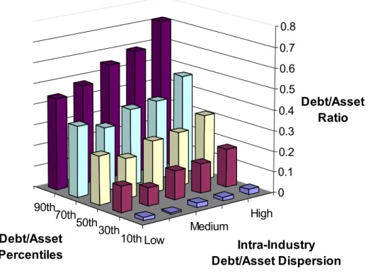
Figures 1a and 1b show the extent of variation in financial structure by grouping industries into quintiles based on intra-industry dispersion in financial leverage. We average each firm’s debt-to-asset ratio over all years it appears in the panel and then measure dispersion by calculating the standard deviation of these average debt-to-asset ratios across firms in each four-digit SIC industry. We sort industries into dispersion quintiles and form financial-leverage quintiles within each of these dispersion quintiles. Figure 1a plots financial-leverage quintile medians by dispersion quintile.
13
Figure 1b shows the same breakdown for one specific year, 1990, arbitrarily chosen from the middle of our panel, to establish that averaging over time does not materially change the patterns we observe. Both figures clearly show that there is substantial financial-structure dispersion within four-digit SIC industries, even within industries with the least dispersion.
To give a more concrete idea of the types of industries found in our sample, Table I presents the top ten and bottom ten industries in terms of financial-structure dispersion. As above, we measure dispersion as the standard deviation of firm financial leverage (for each industry) where firms’ debt-to-asset ratios are first averaged over time to form a single measure of financial leverage for each firm. Similar to Figures 1a and 1b, Table I shows that the extent of dispersion is high within industries, and that even industries with the least dispersion exhibit wide intra-industry variation.
Insert Table I here B) Summary Statistics
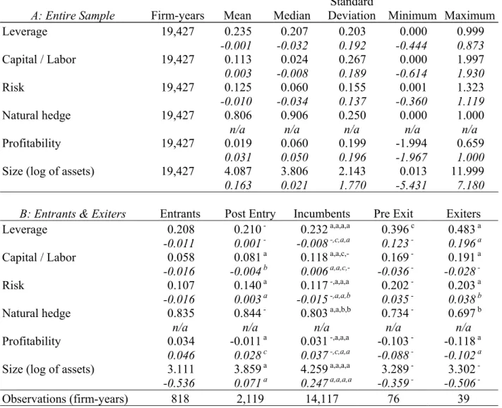
Table II reports summary statistics for six key variables in our analysis that are emphasized in industry equilibrium models: financial leverage, capital-labor ratios, cash-flow volatility, natural hedge, profitability, and asset size. To examine the dynamic predictions formulated by Williams (1995) and Fries et al. (1997), we present results for the entire sample (panel A), entrants and exiters
versus incumbents (panels B & D), and switchers and sellers versus incumbents (panels C & D). We distinguish entrants from switchers, and exiters from sellers, because we suspect that by creating or destroying productive capacity, true entry and exit have a deeper impact on industry equilibrium than entry and exit through acquisition or sale of existing assets, which merely reshuffle the ownership of productive capacity.10 We report raw values in all the panels but focus on the industry-year adjusted
statistics presented in italics since we are primarily interested in within-industry patterns.
10 Data limitations prevent us from precisely determining the type of firm entry. For instance, we cannot distinguish between privately-held incumbents that go public and new firms that actually add productive capacity to their industry. We should point out that by tracking firms by their CRSP permanent number (permno) rather than by their COMPUSTAT CUSIP, we avoid miss-classifying firms that undergo mergers and acquisitions or name changes as entrants. By using the historical SIC from CRSP rather than the current SIC from COMPUSTAT, we can identify incumbent firms that change industry. Thus, we refer to firms that change two-digit SIC industry between the 1981-1990 and 1991-2000 subpanels as “switchers”. Finally, thanks to COMPUSTAT’s “reason for deletion” variable (footnote 35), we are able to distinguish between firms that exit through Chapter 11 bankruptcy or Chapter 7 liquidation and those whose assets are simply redeployed through corporate restructuring.
14 Insert Table II here
Panel A shows that there is wide variation in financial structure and all the other variables, both in raw levels and in industry-year adjusted levels. The central column of Panel B shows that, both in industry-year adjusted and unadjusted terms, incumbents are statistically and economically larger (by a factor of ten) than entrants and exiters.11 Comparing entrants and incumbents, we find
that entrants are smaller, less capital-intensive firms. Entrants and incumbents are equally profitable, but entrant profitability drops significantly in the years following entry. Except for size, exiters are very different from entrants: exiters are twice as financially leveraged, four times more capital-intensive, and highly unprofitable, both prior to and upon exit. These results are consistent with Williams (1995) who predicts that, in equilibrium, industries comprise a core of large, profitable, capital-intensive, financially-leveraged incumbents, flanked by a fringe of small, unprofitable, labor-intensive firms operating at the margin of the industry, i.e., entrants and exiters. However, the Williams equilibrium does not allow for factors such as financial distress, which may well explain why exiters accumulate debt prior to exit, pointing to a limitation of the Williams model.
Entrants and exiters differ in how their technology compares to the rest of their industry. Entrants begin their existence with capital-labor ratios that are significantly closer to the industry median than the average incumbent firm (natural hedge of 0.835 for entrants versus 0.803 for incumbents). Although their greater natural hedge theoretically shields entrants from industry shocks, we find that, in practice, entrants’ cash-flow volatility is not significantly different than incumbents’. Exiters end their existence with capital-labor ratios that are significantly further from the industry median than the average incumbent (natural hedge of 0.697 for exiters versus 0.802 for incumbents) and risk levels about twice as high as incumbents and entrants. This is consistent with Maksimovic and Zechner’s (1991) prediction of an inverse relation between risk and natural hedge. However, exiters’ drop in capital intensity might simply reflect distress as they cut back employment prior to exit. Because this could cause our natural hedge measure to misleadingly correlate with financial distress, we include controls for financial distress in the multivariate regressions that follow.
11 Note that the means for entrants and exiters only reflect the very first or very last year the firm is in the sample. The post-entry column shows means for entrants in the years (up to nine) following the firm’s first year. The pre-exit column shows means for pre-exiters in the years (up to nine) preceding the firm’s last year.
15
The post-entry and pre-exit columns of Panel B report sample means for the years following entry and preceding exit. Both in industry-year adjusted and unadjusted terms, these columns show that entrants generally trend toward incumbent averages while exiters trend away. The evolution of firm characteristics we observe in this sample, namely, entrants’ lower profitability and higher risk levels following entry, resemble the equilibrium outcome modeled in Williams (1995) which explicitly considers how capital-market imperfections limit entrants’ financial leverage, capital intensity, and overall size, putting them at a disadvantage relative to incumbents.
Panel C of Table II reports mean firm characteristics for the first year and years following entry by switchers (switch and post-switch), and for the last year and years preceding exit by sellers (sell and pre-sell). Consistent with the idea that true entry and exit have a deeper impact on industry equilibrium than entry and exit through acquisition or sale of existing assets, we find similar but smaller differences between switchers, incumbents, and sellers than the differences observed in Panel B between entrants, incumbents, and exiters. We find that, unlike entrants, switchers are significantly more risky, less profitable and further from median industry capital-labor ratios than incumbents. The time path observed between entry and post entry and between pre exit and exit is also evident here: Switchers generally move toward incumbent-firm characteristics whereas sellers trend away.
C) Decomposing the Variation in Financial and Real-Side Characteristics
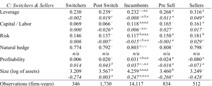
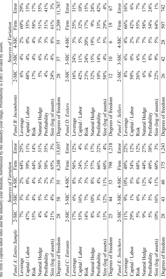
Table III uses analysis of variance to examine the importance of industry and firm fixed effects in explaining financial leverage, capital-labor ratios, cash-flow volatility, natural hedge, profitability, and asset size. We use nested industry dummies to determine the relative importance of two-, three-, and four-digit SIC industry fixed effects. We include firm dummies to contrast between- and within-firm variation (the latter corresponds to the error term reported in the last column of each panel of the table). We present these results for the entire sample and for subsamples of firms that enter, stay, or leave their industry over the course of the panel period (1981-2000).
Insert Table III here
Panel A (entire sample) shows that, except for capital-labor ratios, firm fixed effects rather than industry fixed effects are the main source of cross-sectional variation. In particular, firm fixed
16
effects account for 64% of the variation in financial leverage. Industry effects account for only 11% of the variation, most of which is explained by two-digit SIC industry effects.12 In other words, most
of the variation in financial structure arises within industries rather than between industries.
In contrast to the results for financial leverage, industry effects explain a large share of the variation in capital-labor ratios (50%), mainly at the two-digit SIC level (47%). Thirty-nine percent of the variation in capital-labor ratios is explained by firm fixed effects, and 11% is within-firm variation. These results suggest that capital intensity is highly industry-specific, with some variation across firms but little change at the firm-level over time. These findings are consistent with capital intensity being essentially fixed once technology is chosen. They also suggest that two-digit industry dummies are reasonable proxies for capital intensity.
The sources of variation in cash-flow volatility are similar to those driving financial-leverage variation, with a stronger industry component (23% versus 11%) and less within-firm variation (14%
versus 25%). Natural hedge variation is 12% industry-specific, 56% firm-specific, and 31% within-firm. The breakdown of profitability variation is almost identical to that of natural hedge. Variation in asset size is 32% industry-specific but still mostly firm-specific (65%), and very persistent over time (only 3% unexplained within-firm variation).
Panels B through F of Table III present industry and firm effects for incumbents, entrants, exiters, switchers, and sellers. We find that for exiting firms especially, but also for entering firms, industry effects are substantially more important than for the entire sample or incumbent firms. For example, among entrants (switchers) industry factors explain 31% (30%) of the variation in financial leverage versus only 11% (12%) for the entire sample (incumbents). For exiters, industry fixed effects actually dominate firm fixed effects, suggesting that industry shocks affect these firms more strongly than other firms within a given industry. This conclusion is supported by Maksimovic and Phillips (1998) who show that industry shocks are one of the most important factors influencing the incidence of Chapter 11. Finally, the greater role of firm effects among incumbents relative to other
12 For a direct comparison with Bradley, Jarrell, and Kim (1984), we perform an unreported analysis of variance by collapsing the data into firm-specific averages for the panel period. Our conclusions are basically unchanged: The industry breakdown is 8% (2-digit SIC), 3% (3-digit SIC), and 3% (4-digit SIC) of variation in financial leverage. We also find that year effects by themselves explain less than one percent of the variation in these six variables.
17
subsamples broadly supports Williams’ (1995) idea that firms operating at the core of their industries (incumbents) differ substantially from those at the fringe (firms that enter and leave their industries).
D) Influence of Industry on Firm Financial Structure
Our analysis of variance established the relative unimportance of industry in explaining firm-level financial structure. We now supplement our analysis of variance with a more parametric approach that explores the relation between firm-level and industry-level financial structure, firm responses to changes in industry financial structure, and firm reversion to industry financial structure.
Insert Table IV here
Table IV shows regressions of firm-level financial structure on various measures of industry-level financial structure. As in our analysis of variance, where we use nested dummy variables, we avoid overlapping industry and firm effects by excluding firms at finer industry definitions from the calculation of more broadly-defined industry means. For instance, mean four-digit SIC industry financial leverage for a firm in SIC 3561 excludes that firm. Mean three-digit SIC industry for this firm excludes firms in SIC 3561, and its two-digit SIC industry mean excludes firms in SIC 356.13
Panel A of Table IV tests the relation between industry and firm-level financial structure by regressing firm-level debt-to-assets ratios on lagged industry median and mean debt-to-assets ratios. We lag the industry debt-to-assets ratios to avoid endogeneity problems.14 We present median and
mean industry regressions to check whether influential observations affect our results. This leads to some differences in findings but not in the overall conclusions. Consistent with our analysis of variance, we find strongest significance at the two-digit SIC industry level, and the adjusted R-square ignoring firm fixed effects is under ten percent but climbs to 66 percent when firm fixed effects are included. Thus, as the magnitude of the coefficients and adjusted R-square statistics show, the ability of industry to explain financial structure is limited and is in fact overshadowed by firm fixed effects.
13 This causes the degrees of freedom to drop from 19,426 in Table III to 19,374 in Table IV. This is because some three-digit SIC industries contain a single four-digit SIC industry.
14 Even if we estimate these relations using contemporaneous medians and means for industry financial structure, the adjusted R-square only increases by one percentage point for the industry-medians regression and two percentage points for the industry-means regression.
18
Panel B tests how firms respond to changes in industry-wide financial structure by regressing changes in firm debt-to-assets ratios on concurrent changes in industry debt-to-assets ratios. Our results are qualitatively similar for changes in industry medians and means, though weaker for the latter. Although we find statistical significance at the two- and four-digit SIC level, the low R-squares (2% for medians and 1% for means) suggest that firms adjust their financial structures very little in response to their industries, consistent with our findings in Table III that both broadly- and narrowly-defined industries explain a rather small share of firm-level variation in financial leverage.
Finally, Panel C examines firm reversion to industry financial structure by regressing changes in firm assets ratios on lagged differences between firm and mean industry debt-to-assets ratios (similar findings also obtain using the median industry debt-to-asset ratio). We also present a semi-parametric version that uses the decile ranks rather than the actual values of the lagged differences between firm and mean industry debt-to-assets ratios. The two methods concur qualitatively, showing that firms do revert to industry debt-to-assets ratios. However, this reversion occurs at a very slow rate. We find annual industry-mean reversion rates of 5.0% for two-digit, 5.2% for three-digit, and 7.0% for four-digit industries, not unlike Fama and French (2002) who report that firms revert to their own leverage targets at rates of 7% to 18% per year. This evidence of slow mean reversion is consistent with Fischer, Heinkel, and Zechner (1989), suggesting that there are substantial transaction costs in adjusting firm financial structure. However, it is also consistent with industry equilibrium outcomes where firms do not rapidly adjust toward the industry mean but rather adopt differential financial structures that persist over time within their industry, consistent with our analysis of variance results and findings described in the sections which follow.
E) Intra-Industry Covariance Patterns
Table V continues our analysis of intra-industry variation by presenting quintile means.15 We present these quintiles to detect nonlinear relations across firms within industries and investigate the predictions advanced by Maksimovic and Zechner (1991) and Williams (1995) regarding the equilibrium structure of industries along the dimensions of debt, technology, and risk. For instance,
19
Maksimovic and Zechner predict that firms with atypical technologies carry more debt and exhibit more risk. If this prediction holds, we should observe non-monotonic relations between financial leverage, capital-labor ratios, and cash-flow volatility. A standard correlation analysis would not allow us to detect the non-monotonic relations predicted by these studies.
We construct industry-year quintiles for key regressors featured in our multivariate regressions (natural hedge, asset size, and profitability) and compute quintile means for these variables and our three dependent variables (financial leverage, capital-labor ratios, and cash-flow volatility). Quintiles are formed for each of the 142 four-digit SIC industries in each of the 18 sample years (2,556 industry-years).16 We report industry-year adjusted quintile means as we wish to focus
on within-industry distribution patterns. Having said this, our conclusions are generally unchanged with or without industry-year adjustments, and most of the quintile means differ significantly in both cases. To give a better idea of the economic significance of these industry-year adjusted quintile means, we also present mean sample percentile ranks in parentheses.
Insert Table V here
The top panel of Table V shows how each of our key variables distributes across the first, third, and fifth natural-hedge industry-year quintiles. We find a U-shaped relation between financial leverage and natural hedge, and a monotonic inverse relation between risk and natural hedge. These findings lend mixed support to the monotonic inverse relations Maksimovic and Zechner (1991) predict between financial leverage and cash-flow volatility and a firm’s proximity to the mainstream industry technology. The relation between asset size and natural hedge is also U-shaped, indicating that, contrary to what Williams (1995) predicts, large firms operate not only at the technological core of their industries but also at the fringe, in other words, with both low and high capital-labor ratios. Because many of these relations are non-monotonic, we include the squared value of natural hedge in our multivariate regressions.
The middle panel of Table V shows how the same six variables distribute across profitability quintiles. The relation between financial leverage and profitability first decreases slightly
20
year adjusted means of 0.03 and 0.02 for quintiles one and three), then falls steeply (-0.07 in quintile five). Although our finding of an inverse relation is consistent with existing findings (Long and Malitz, 1985, Rajan and Zingales, 1995, Graham, 2000, and Fama and French, 2002), the fact that financial leverage, capital-labor ratios, and cash-flow volatility are all nonlinearly related to profitability leads us to include the squared value of profitability in our multivariate regressions.
The bottom panel of Table V reports means by asset size quintile. Consistent with a Williams-style core-fringe industry structure, we find that financial leverage, capital intensity, and profitability all increase in size. Interestingly, even though the largest firms are significantly less like their industry than small firms (natural hedge of 0.77 for the top size quintile versus 0.82 for quintile one), large firms are much less risky than small firms. This suggests that although natural hedge reduces risk in principle, in practice, this effect is overshadowed by other determinants of firm risk.
Finally, we refined the analysis presented in Table V by splitting the industries based on intra-industry dispersion. We contrast low- and high-dispersion industries because in some industries the scope for technological variation might be limited, making it difficult to detect relations between the variables. We do not report this analysis, as the results were substantially the same as those shown in Table V. They are simply accentuated in high-dispersion industries.
F) Evolution of Entrants, Exiters, Switchers, Sellers, and Incumbents within Industries
To investigate the dynamic properties of industry equilibrium, as modeled by Williams (1995) and Fries et al. (1997), Table VI presents transition frequencies for firms that enter, stay, or leave their industries. For each variable presented, the table panels show the percentage of incumbent firms that stay in the same industry-year quintile or move to other quintiles between the first half of the empirical period (1981-1990) and the second half (2000). Each panel also shows the 1990-2000 quintile distribution of firms that enter an industry in the 1990-1990-2000 time period, either through new entry (enter) or by changing two-digit SIC industry (switch). Finally, the panels show the 1981-1990 quintile distribution of firms that leave an industry in the 1981-1990-2000 time period, either through bankruptcy or liquidation (exit) or by selling assets through corporate mergers or acquisitions (sell). The quintiles are formed using firm means for each time period (1981-1990 and 1990-2000). The
21
table also reports statistical tests of differences in proportions between the first, third, and fifth quintiles, and goodness-of-fit tests that industry demographics follow a Uniform distribution.
Insert Table VI here
We note several transition patterns for incumbent firms and for firms that enter or leave their industries. First, the top-left panel of Table VI shows that 23% of entrants fall in the lowest financial-leverage quintile. This percentage falls significantly to 18% in quintiles three and five. In contrast, switchers tend to enter an industry in the higher financial-leverage quintiles, with 24% and 22% of switchers in the fourth and fifth quintiles. Among exiters, seven times more firms belong to the top financial-leverage quintile than the bottom quintile. This pattern also obtains for sellers, though in a less dramatic but still significant proportion of 37% to 28%. Since most of the quintile frequencies pertaining to entrants, switchers, sellers, and exiters concur with the section IV.B discussion of firm means reported in Table II, we now turn our attention to the behavior of incumbent firms over time.
The diagonal elements of each panel represent incumbent persistence rates showing the percentage of incumbent firms that remain in their industry quintile between the 1981-1990 time period and the 1990-2000 time period. For all variables, we find that persistence is greatest for quintiles one, five, or both. This may simply reflect the fact that these quintiles contain the tails of the distribution for each variable: Firms in these quintiles must change substantially to transit to the inner quintiles. The highest persistence rates are 38%, 31%, and 52% for the fifth quintiles for capital-labor ratios, profitability, and asset size, and 44% and 42% for the first asset-size and risk quintiles. These results suggest that large, capital-intensive, profitable, stable incumbent firms tend to maintain their dominant industry position over time, and represent a Williams-style industry core. Higher turnover rates and lower persistence rates arise as capital intensity, profitability, and asset size decrease, and as financial leverage and cash-flow volatility increase. These results suggest that small, labor-intensive, unprofitable, risky, marginal firms tend to move in, around, and out of their industries over time, and represent a Williams-style industry fringe.
We find for all variables persistence rates that significantly diverge from 20%, the rate expected if incumbents were uniformly randomly redistributed across quintiles between 1981-1990
22
and the 1990-2000 time period. Consistent with our industry-mean reversion analysis (Table IV), this finding suggests that firm characteristics evolve slowly and that firms maintain their relative industry positions, even within competitively-structured industries. Table VI also highlights the high attrition rate among small firms (fully 41% of firms in the lowest asset-size quintile sell out, 3% exit, and 44% remain in the lowest asset-size quintile) and the staying power of large firms (52% of firms in the highest asset-size quintile remain in that quintile, 1% exit, and 20% sell out).
G) Multivariate Analysis of the Relation Between Financial Structure, Technology, and Risk
Although informative, the evidence uncovered so far in support of industry equilibrium models relies on univariate analyses. In this section, we use multivariate regressions to determine whether this evidence holds up in a simultaneous-equation framework that controls for covariates and deals with endogeneity in the regressors and simultaneity between three dependent variables featured in industry equilibrium models: financial leverage, capital-labor ratios, and cash-flow volatility.
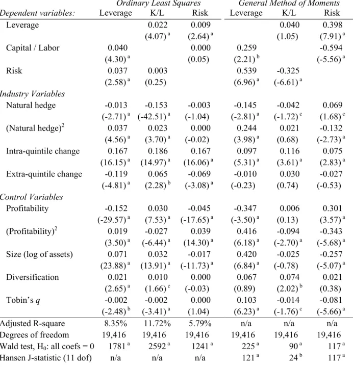
Table VII presents Ordinary Least Square (OLS) and General Method of Moments (GMM) regression results. In contrast to OLS, GMM allows for simultaneity among the dependent variables by incorporating the correlation of residuals across the three equations. This improves the efficiency and consistency of the estimates. Moreover, as an instrumental-variable estimation method, GMM mitigates simultaneity bias caused by endogenous explanatory variables by using predicted values rather than realized values of the variables. We instrument all the regression variables by their second lags in levels and the current and once-lagged intra- and extra-quintile change variables. Hansen’s (1982) J-statistic jointly tests that the model is well-specified and that the instruments are valid.
The panel nature of our sample allows us to control for unobserved firm-specific factors. Instead of the standard deviation-from-means approach, which is invalid when using lagged variables as instruments, we control for firm fixed effects by differencing the variables. However, first-differencing introduces first-order moving-average autocorrelation, so we use the Newey-West
23
(1987) procedure to address this issue and also handle heteroscedasticity. To focus on intra-industry variation, we include dummy variables to control for four-digit SIC industry and year fixed effects.17
Insert Table VII here
We find several differences between the OLS and GMM coefficient estimates, suggesting that resorting to instrumental-variable, simultaneous-equation estimation methods is important. We find that the relation between financial leverage and Tobin’s q flips from highly significant negative
for OLS to highly significant positive for GMM. This sign reversal is not a focus of this study since we simply regard Tobin’s q as a control variable. However, it does suggest that the simultaneity of financial leverage and Tobin’s q is a real issue and requires proper econometric treatment. The other sign reversals we observe between OLS and GMM occur in the capital-labor ratio and cash-flow volatility regressions discussed below. As discussed in the following section, we also find important differences in economic significance between OLS and GMM. Since the GMM estimates are econometrically superior, we focus our discussion on these results.
Inspection of the GMM results for financial leverage (column four of Table VII) shows that financial leverage is positively related to capital-labor ratios, cash-flow volatility, asset size, and Tobin’s q. The relation between financial leverage and cash-flow volatility is of particular interest as past empirical work has in turn found this relation to be positive (Kim and Sorensen, 1986), negative (Bradley, Jarrell, and Kim, 1984), and insignificant (Titman and Wessels, 1988). Besides lending credence to Maksimovic and Zechner’s (1991) prediction of a positive relation between financial leverage and risk, our findings also suggest that the mixed results in the literature might depend on the econometric treatment of simultaneous decision variables and endogenous explanatory variables.
As discussed previously, we construct a number of unique variables to test central predictions of the industry equilibrium models reviewed earlier. One of these is natural hedge, which measures how far a firm’s capital-labor ratio departs from the industry-year median. We find a significant inverse relation between this variable and financial leverage, supporting the Maksimovic and
17 Our results do not hinge on how finely we define industries. Unreported regression results using two- and three-digit SIC industries to measure natural hedge and intra- and extra-quintile changes and to adjust for industry were qualitatively similar and, perhaps thanks to larger sample sizes, statistically stronger. This suggests that the forces which explain the distribution of firms within industries operate at several levels within the overall economy.
24
Zechner (1991) prediction that high-debt firms choose technologies unlike the industry mainstream. Consistent with the finding in Table V of a U-shaped relation between financial leverage and natural hedge, we find a significant positive coefficient for the squared value of natural hedge. This non-monotonic relation is not predicted by Maksimovic and Zechner and suggests that other factors besides those analyzed in their model induce firms at the technological core of the industry to assume more debt than firms whose capital-labors ratios lie between the core and fringe of the industry.
One possibility is that our natural hedge measure acts as a proxy for financial distress. As discussed earlier, we observe an increase in capital intensity prior to firm exit (see Table II), arguably because exiting firms enact cost-cutting measures such as cutting back employment. Thus, because it is constructed from capital-labor ratios, the natural hedge for exiting firms will reflect this behavior and trend lower prior to firm exit. We use two methods to avoid confusing financial distress with a
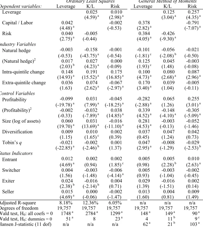
bona fide natural hedge effect. First, we include capital-labor ratios themselves in the financial leverage regressions; we also control for risk, profitability, and size, which Table II showed to be good exit predictors and indicators of financial distress. Second, we run separate regressions (Tables IX and XI) that include dummy variables for exiting firms.
Another implication of the industry equilibrium models is that even in competitive industries, decisions made by individual firms are not independent of the decisions made by the rest of the industry. Consequently, our regressions also include the mean change in the dependent variables both inside and outside a firm’s industry-year quintile (intra- and extra-quintile change) as another empirical strategy to detect intra-industry linkages.18
We find significant positive relations between the intra-quintile change variables and each of the three dependent variables. The OLS results show that firms make financial and risk adjustments inversely related to those of firms outside their quintile. However, these results do not hold up statistically under GMM. These findings, that firms behave like (unlike) firms inside (outside) their industry-year quintile, support the asymmetric adjustment patterns predicted by Maksimovic and
18 Intra-quintile change is the mean change in the dependent variable within the firm’s own industry-year quintile. To avoid hardwiring a positive but spurious relation into the analysis, we exclude each firm from its industry-year quintile in calculating the intra-quintile mean change. Extra-quintile change is the mean change outside the firm’s industry-year quintile. The quintiles themselves are based on the lagged levels of the dependent variables.
25
Zechner (1991). Our finding that firms’ actions are correlated with the actions of other firms in their own industry-year quintile suggests that strategic complementary usually associated with imperfect competition arises even within competitively-structured industries.
Contrary to the heuristic that real and financial leverage are inversely related, but directly supporting a Williams (1995) prediction, we find that financial leverage is increasing in capital intensity.19 Interestingly, column five of Table VII shows that causation does not run both ways: The
relation between capital intensity and financial leverage is positive but not significant. The OLS results fail to make this distinction, leading one to conclude that causation runs both ways. In fact, the OLS results suggest that capital intensity is significantly related to all the regressors except diversification. Many of these relations are insignificant under GMM, attesting to the simultaneity of capital intensity and the regressors, and the importance of instrumental-variable estimation in removing simultaneity bias and reducing spurious associations.
Finally, column six of Table VII confirms the positive relation between risk and financial leverage found in the first equation and the inverse relation between risk and capital intensity found in equation two. It also shows that cash-flow volatility is directly (inversely) related to profitability (squared), and inversely related to Tobin’s q. These results are the opposite of those we find under OLS (column three), again pointing to how simultaneity bias can lead to erroneous conclusions.
Although we have argued that instrumental-variable estimation addresses endogeneity issues, we have not yet discussed whether our instruments remove simultaneity bias altogether. As commonly happens, Table VII shows that the Hansen J-statistics strongly reject the over-identifying restrictions in every GMM equation.20 This could mean that the model is misspecified, that the
instruments are correlated with the residuals, or that both violations occur.21 Experimentation with
19 This might also obtain if capital intensity is a proxy for collateral assets and thereby increases debt capacity. However, this interpretation is insufficient given that we control for collateral effects by including total assets. 20 The GMM results reported in Table VII are from a simultaneous estimation of the regression equations, yielding a
single J-statistic for the system of equations, which also strongly rejects the over-identifying restrictions. We produce the equation-specific J-statistics reported in table VII by estimating each equation individually.
21 However, J-tests hold asymptotically and are known to over-reject in finite samples (Ferson and Foerster, 1994). Moreover, as Stock and Wright (2000) discuss, this problem worsens when the instruments are weakly correlated with the endogenous variables. Finally, Leamer (1983) shows that large-sample specification tests are sensitive even to small departures from the “true” model.
26
different model specifications and other sets of instruments neither improved the J-statistics nor fundamentally altered our results. Thus, although the variables are instrumented with plausible instruments, we cannot say for sure that even our GMM estimates are free of simultaneity bias.
H) Economic Significance
Table VIII shows the economic significance of the regression results reported in Table VII. The table presents predicted percentage changes in the dependent variables as each regressor varies from the 5th to 95th percentile holding all other regressors at their sample mean levels (statistically
insignificant relations are omitted). The percentages we report are relative to the sample range (maximum less minimum). Panel A (B) uses the OLS (GMM) coefficient estimates from Table VII.
Insert Table VIII here
Table VIII shows that, except for intra-quintile change, all the variables exhibit substantially more economic significance under GMM than for OLS. Given the econometric issues mentioned earlier, we focus on the GMM version of the economic significance results. Panel B shows that the economically most significant determinants of financial leverage are: asset size (going from the 50th
to the 5th (95th) asset-size percentile coincides with a 8.1% (10.9%) drop (rise) in financial leverage),
Tobin’s q (going from the 50th to the 5th (95th) Tobin’s q percentile coincides with a 6.3% (7.0%)
drop (rise) in financial leverage), profitability (going from the 50th to the 5th (95th) profitability
percentile coincides with a 4.1% (3.3%) drop (fall) in financial leverage), and natural hedge (going from the 50th to the 5th (95th) natural-hedge percentile coincides with a 2.4% (1.3%) rise (drop) in
financial leverage). This last finding confirms that an economically significant fraction of within-firm variation in financial structure is tied to industry factors other than standard industry fixed effects.
The economic impact that natural hedge and profitability have on financial leverage is complicated by the non-monotonic relations between these variables and financial leverage. Indeed, Table VII shows negative coefficients for both variables and positive coefficients for their squared values, all statistically significant under OLS and GMM alike. Thus, the overall economic impact that natural hedge and profitability have on financial leverage reflects these opposing signs. Combining these offsetting relations, both panels of Table VIII concur in showing that, consistent