A molecular dynamics study of the microscopic properties of simple dense fluids

PROPERTIES OF SIMPLE DENSE FLUIDS

Thesis by

Paul Lee Fehder

In Partial Fulfillment of the Requirements For the Degree of

Doctor of Philosophy

California Institute of Technology Pasadena, California

1970

ACKNOWLEDGMENTS

I wish to express my sincere appreciation to those individuals and organizations who have contributed so much to this research, and to my personal happiness and well-being during my tenure at

CalTech--Professor G. W. Robinson, my research advisor, for his inter-est, encouragement, and support over the four years during which this research was being pursued. Were it not for his generosity and

personal flexibility, such a project could not even have been initiated. Dr. R. P. Futrelle, who has been most instrumental in intro-ducing me to the mysteries of modern classical statistical mechanics. His helpful suggestions and enlightening hints have been a significant contribution to my research efforts.

Dr. C. A. Emeis, a most worthy colleague. His ability to enter into an unfamiliar field of research, and within the short span of a year to make several important contributions to that research effort, is indeed commendable.

Professor C. J. Pings, whose expressions of interest and

encouragement seemed always to come at just the right time to assuage my occasional sense of frustration. Professor Pings and Dr. S. C. Smelser are most responsible for rekindling my interest in the radial distribution functions computed from the simulation data.

Professor F. B. Thompson, who has done a great deal to broaden my thinking with respect to the scientific application of auto-matic data processing.

Frank Rouser, Kiku Matsumoto, Joe Daly, Dallas Oller, and other members of the Booth Computing Center staff; their assistance has been invaluable in finding solutions to a number of rather knotty programming problems.

The C. I. T. Chemistry Department provided the "seed money" to support the initial phases of this research; the bulk of the project was supported by grants from the National Science Foundation.

Personal financial support was provided by the Chemistry Department, NSF, E. I. du Pont de Nemours and Company, and through summer grants by the Shell Company Foundation and American Cyanamid. I would especially like to thank du Pont for its generosity during the 1967-68 academic year; the (relative) munificence of the du Pont Award for Postgraduate Teaching permitted me to discover many of the finer aspects of life in Southern California. I would also like to thank my parents, Mr. and Mrs. Lee G. Fehder, for their frequent "grants--in-aid" during times of financial stress.

ABSTRACT

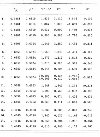
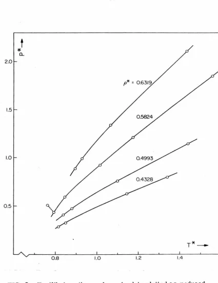
The microscopic properties of a two-dimensional model dense fluid of Lennard-Jones disks have been studied using the so-called "molecular dynamics" method. Analyses of the computer-generated simulation data in terms of "conventional" thermodynamic and distribu-tion funcdistribu-tions verify the physical validity of the model and the simuladistribu-tion technique.

The radial distribution functions g(r) computed from the simula-tion data exhibit several subsidiary features rather similar to those appearing in some of the g(r) functions obtained by X-ray and thermal neutron diffraction measurements on real simple liquids. In the case of the model fluid, these "anomalous" features are thought to reflect the existence of two or more alternative configurations for local ordering.

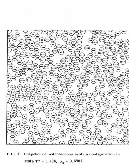
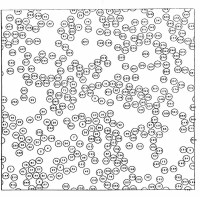
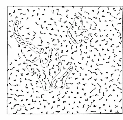
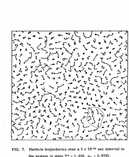
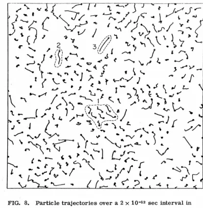
Graphical display techniques have been used extensively to pro-vide some intuitive insight into the various microscopic phenomena occurring in the model. For example, "snapshots" of the instantaneous system configurations for different times show that the "excess" area allotted to the fluid is collected into relatively large, irregular, and surprisingly persistent "holes". Plots of the particle trajectories over intervals of 2. 0 to 6. 0 x 10-12 sec indicate that the mechanism for dif-fusion in the dense model fluid is "cooperative" in nature, and that extensive diffusive migration is generally restricted to groups of particles in the vicinity of a hole.

predictions of existing theories of singlet, or self-diffusion in liquids. The relative diffusion of proximate particles is, however, found to be retarded by short-range dynamic correlations associated with the cooperative mechanism- -a result of some importance from the stand-point of bimolecular reaction kinetics in solution.

A new, semi-empirical treatment for relative diffusion in liquids is developed, and is shown to reproduce the relative diffusion phenomena observed in the model fluid quite accurately. When incor-porated into the standard Smoluchowski theory of diffusion-controlled reaction kinetics, the more exact treatment of relative diffusion is found to lower the predicted rate of reaction appreciably.

TABLE OF CONTENTS

I. INTRODUCTION

A. Some General Comments Regarding the Liquid State • • • • • • • • • • • • • B. A Brief Outline of Theories of the Liquid

State . . . .

. . . .

. .

. .

Formal Theories

. .

. . .

.

.

.

. .

Superposition Approximation PY Equation • • . • • • • "Scaled-Particle" Method

. . .

.

. .

Model Theories. • • • • . . Cell Theory • . • • • . Hole Theory • • • . • Cell-Cluster Theory •

Tunnel Theory

Significant Structure Theory

.

. .

.

. . .

.

.

. .

C. A Review of Molecular Dynamics Studies at

Other Laboratories

.

.

. .

.

. . .

.

.

.

.

.

D. An Informal Description of the Approach Taken

in This Research. REFERENCES. • • •

II. TECHNICAL DESCRIPTION OF METHODS AND PROCEDURES

A. The Basic Molecular Dynamics Algorithm

B. Equipment . . . • . . • . • . C. Implementation of the Algorithm

Page

35

35

D. Auxilliary Procedures • • • • • • 44 III. CONVENTIONAL ANALYSES OF THE SIMULATION DATA

A. Introductory Comments

.

. . .

. .

.

. .

. .

50 B. Paper No. 1: Molecular Dynamics Studies of the

Microscopic Properties of Dense Fluids •

52

C. Notes and Addenda to Paper No. 1. • . 94 D. Paper No. 2: "Anomalies" in the Radial

Distribution Functions for Simple Liquids 97 E. Notes and Addenda to Paper No. 2. • • . 124 IV. DIFFUSION, RELATIVE DIFFUSION, AND CHEMICAL

REACTION KINETICS IN DENSE FLUIDS A. Introductory Comments • • • . • •

B. Paper No. 3: The Microscopic Mechanism for Self-Diffusion and Relative Diffusion in Simple

Liquids . . . . C. Paper No. 4: The Microscopic Mechanism for Diffusion, and the Rates of Diffusion-Controlled Reactions in Simple Liquid Solvents . . . • . . V. FORMAL LANGUAGE FOR THE DESCRIPTION OF

LIQUID STRUCTURES--A PROPOSAL A. Explanatory Comments . . B. Statement of the Problem •

127

129

179

C. A Formal Language of Partially-Ordered Structures • • • • • • • • . • • • • D. The Radial Distribution Function g(r) E. Geometrical Neighbors. .

F. Discussion VI. PROPOSITIONS

.

.

.

Proposition 1: Elucidation of the Role of S0₂ in Atmospheric Aerosol Formation Proposition 2: A Spectroscopic Search for an

HgCO Complex . • • . • . .

Proposition 3: Improvements on the Photochemical Space Intermittency Method for Measuring the Diffusion Coefficients

Page

211 214 216 219

224

237

of Free Halogen Atoms in Solution • 246 Proposition 4: A Molecular Dynamics Study of Cavity

Formation Works in a Simple Liquid. 263 Proposition 5: An Examination of Solute Diffusion

as a Function of the Relative Sizes and Masses of the Solute and Solvent

SECTION I

A. Some General Comments Regarding the Liquid State

The foundations for our physical understanding of the vapor state were established during the eighteenth and early nineteenth centuries. 1 And somewhat more recently, x-ray and now thermal neutron diffraction measurements have provided extremely detailed information regarding the microscopic structures of a large number of crystalline solids. But the liquid state, occupying as it does a kind of "middle ground" between solids and gases, is undoubtedly more complex and less well under-stood than either.

The solid state is stable at low temperatures and/or high pres-sures, is characterized by high cohesion and rigidity, and at the molecular levels exhibits a high degree of (crystalline) order and structure. Gases are stable at low pressures and high temperatures, are characterized by low cohesion, a complete lack of rigidity and low resistance to flow, and to a good approximation are entirely devoid of structure or order at the molecular level. The liquid state is stable over an intermediate range of temperatures and pressures, and is characterized by a high cohesion, a lack of rigidity, and a comparatively low resistance to flow.

relatively small increase in volume (of the order of 12% for the solid inert gases), and thus the spatial arrangement of the atoms or molecules in a liquid must--at least in the region of the melting point--bear some similarity to the crystalline structure of the corresponding solid. This proposition is also supported by the well-known experimental fact that the latent heat of fusion is always much smaller than the latent heat of vaporization; the cohensive forces between the molecules of a substance must not therefore change appreciably with melting. And finally, we note that the specific heat of condensed bodies is only slightly affected by fusion, indicating that thermal motion in the solid and liquid near the melting point must be fundamentally rather similar.

The ambiguity implied by the macroscopic physical properties of the liquid state is at least partially resolved by the results of x-ray diffraction and thermal neutron scattering measurements. 2 These measurements, in addition to some spectroscopic data, 3 indicate that the liquid state is characterized by a microscopic structure that is essentially neither vapor-like nor solid-like. 4 Rather, liquids are "partially ordered" at the molecular level; that is, the spatial

important, the statistical-geometric techniques necessary to establish a quantitative measure of the "degree" of order in a partially-ordered

structure have not as yet been devised. For a more detailed discussion of this latter point, see the discussion in section V.

Of all the physical sciences, classical chemistry is perhaps most dependent upon an intuitive understanding of the physical phenom-ena it purports to investigate. Organic chemists tend to think of mole-cules as real physical entities comprised of real atoms arranged in a reasonably well-defined spatial configuration--and of chemical reaction mechanisms in terms of the re-arrangement of these configurations during the encounter between two molecules in a reaction medium. This reaction medium is most frequently some liquid solvent; yet, because of the dirth of "practical" information regarding the microscopic processes characteristic of the liquid state, even very "intuitive" descriptions of a chemical reaction mechanism will frequently fail to consider possible dynamic interactions between tne activated complex and molecules of the surrounding solvent. It is true, of course, that the so-called "solvent cage effect" is occasionally called upon to explicate the mechanism for, e. g. , a complicated molecular rearrangement. But even this very simple model for solvent-solute interactions is not well defined, and it appears that different chemists envision the physical processes underlying the "effect" in different ways. Again, the Smoluchowski treatment of diffusion-controlled reaction kinetics in

the "collision" theory of chemical reaction kinetics invokes a "solvent cage" model to explain the observed rates of reactions requiring a

(supposedly) high activation energy or a specific steric orientation for the reactant molecules.

Other chemico-physical phenomena are also interpreted in terms of "operational" models for the liquid state. For example, nuclear spin-lattice relaxation in solution by nuclear-spin-internal-rotation coupling requires a dynamic interaction between the NMR-active solute molecule and the molecules in the surrounding solvent environment. The absorption spectra of atomic mercury dissolved in a variety of (apparently) inert liquids is thought3 to reflect the different types of local solvent environment in which a ground-state solute mercury atom might find itself. But the physical models for these interactions and solvent environments must be viewed with some skepticism until a more definitive model is fashioned for the liquid state itself. And, as we shall see in the next section, present efforts to construct a good theory of liquids do not seem to aspire to the development of such a model.

B. A Brief Outline of Theories of the Liquid State

outline of the approach taken in the development of a representative

sampling of these theoretical treatments; this outline will then serve as a background against which we may contrast the direction and

results of our own research.

For the sake of discussion, the various theories of the liquid state may conveniently be divided into two groups. The "formal" theories of the sort pioneered by Kirkwood and Mayer offer the aesthetic pleasure of initial rigor. But approximations have always been necessary at some point in the development of these theories to make the mathematics tractable, and while most of the approximations are almost assuredly valid from a purely mathematical point of view, the physical implications of a given approximation are often not

immediately obvious.

The theories falling into the second group--the "model" theories are each based on some operational model for the microscopic struc -ture and dynamics of the liquid state. In selecting a given model for

study, the theoretician supposes that: (i) the mathematics deriving

from the model will be tractable without further approximation, and (ii) the model is a reasonable representation of the real liquid. Some simplifying approximations are usually made during the mathematical development of a "model" theory. But these approximations are

The "model" approach to liquid theory offers the advantage that, within the limits of any simplifying approximations, the theoretical formulations developed from a given model are at least a valid

statistical-mechanical treatment of that model. If a "model" theory is capable of reproducing the thermodynamic or equation-of-state data for a real liquid, then it is generally assumed that the model is a reason-ably accurate representation of reality. In fact, however, the thermo-dynamic functions do not serve as a critical test for the validity of a theoretical model; the statistical averaging implicibf in any of the thermodynamic quantities is so extensive that even a patently "naive" model may experience some success in obtaining agreement with experimental data. The transport properties might conceivably serve as a medium for more severe tests of the various theoretical treatments. Unfortunately, most of the models that have been examined are static in nature and do not lend themselves to the calculation of

transport-related quantities.

Formal Theories

~

PV

=

Nk T -

W

fao

r g(r) o<J?(r) 47rr2 dr

B 6V 0

ar

The total internal energy is similarly related to g(r):

2 ao

E

=

~

NkBT +

~

f

g(r) cp(r)' 47rr2 dr 0

From the equation-of-state and total energy, all the thermodynamic properties of the system can be calculated.

Kirkwood, 6 Born and Green, 7 Yvon, 8 and Bogoliubov9 have developed a number of essentially equivalent integral equations for the molecular-pair distribution function n<2_{>(,!:.1' !;i), defined as the} prob-ability of finding an arbitrary pair of molecules in the configuration

(.!:_~, !;i). That is, n<2>(!j., .!:__{2 )} is the probability of simultaneously finding a molecule in the volume element d3r₁ around r₁ and a second molecule

"" ""

in the volume element d3

r.:a

around !;l· Higher-order correlation func-tions n<3>(!j., ~' .!:_3 ), n<

4_{>(,!:.1' ~'}

!:;3' .!:_4 ), etc., are similarly defined. For an isotrop:C fluid, n < 2 > (!j.,

r.:a)

is dependent only upon the scalar distance r12 =

I

!j.2

j

=

I

.!:.i -

~I, and is directly related to the radial distribution function:

2

~

g(r)

and similarly, that on(3)(:£.11 ~' :£_3)/0::£_1 is given by a formula involving

the next higher correlation function n<4_{>(:£_11 :£_2, :£_3, :£_4 ).} Thus to calculate

n<2>--and thence g(r)--we need n<3>; to obtain n<3_{> we need n<}4

>, etc.

To break this chain of linked equations, Kirkwood proposed the

so-called "superposition approximation":

[ n<2>(r12). n<2>(r23). n<2>(r31)]

Po

where p₀

=

N/V is the number density of the system. Born and Green, 7

and Yvon 8 have shown that the equation obtained by substituting the

superposition approximation for n<3> into the equation above for

on(2>(:£_11 ~)/o:£_

1

can be integrated over :£_₁ to obtain:

( nc_2>(r223) - 1 )

Q

r13 -2 ( .r2s - r12 )2] d d

X 2r r23 r23 r13

Po 23

where cp(-r)

=

cp(r) and n<2>(-r)

=

n<2>(r), by definition. Kirkwood and

Bogoliubov obtained slightly different equations using different

Within the limits of accuracy for the superposition approximation,

the BGY equation above and the similar equations obtained by Kirkwood and Bogoliubov each constitute a rigorous (though perhaps not intuitively

enlightening) theory of the liquid state. In fact, the BBGYK equations are found to reproduce the broad features of the radial distribution functions obtained by x-ray diffraction measurements2 on real liquids at moderate densities. For higher densities the superposition approxi-mation begins to fail; in particular, the theoretical distribution functions begin to diverge from the experimental functions just in the regions where cp(r) and acp(r)/ar make the largest contributions to the inte-grands in the formulas for the total energy and equation-of-state.

Perkus and YeVick10 obtained a very different integral equation for g(r) by applying the "method of collective variables. "ll With this

method, disorder in the microscopic structure of a liquid is repre-sented by the superposition of a large number of acoustic waves. The Hamiltonian for the system is then transformed so that, to a good approximation, the configuration integral--and thence the partition function--can be calculated.

where Xn

=

2L/n and n is an integer. N of these collective coordinates,

q 1 ... qN' are required to describe the one-dimensional system.

For real three-dimensional liquids, 3N collective coordinates

are used and the system is assumed to be confined to a cube with edge

dimension L. The reformulation of the Hamiltonian requires a number

of complex mathematical procedures; some of these procedures are

still open to question. Suffice it to say that, using the transformed

Hamiltonian, the partition function and thence all the thermodynamic

properties of the liquid can be calculated.

The Perkus-Yevick treatment leads to the integral equation:

g(r)e q>(r)/kBT

=

1 +Po

J

g(s)

G

-

e q>(s)/kBJ

~(I

s-r

I)-~

ds

for the radial distribution function. Broyles12 has obtained numerical

solutions to this equation for fluids of Lennard-Jones particles at a

number of different temperatures and densities. The resulting radial

distribution functions compare favorably with those calculated using

the Monte-Carlo and "molecular dynamics" simulation techniques--to

a radius of about r

=

1. 5

a.

For larger r the agreement is not quite

so satisfactory, although the results are still much better than those

obtained using any of the BBGYK equations. The PY equation appears

to fail at low densities.

The "scaled particle" method developed by Reiss and

co-workers13 represents potentially yet another "formal" approach to a

theory of the liquid state. The method is based on the idea that, as

molecules that will fit into that void changes discontinuously. The

probability of finding a spherical hole of a given radius in the liquid is

then calculated in terms of the reversible work necessary to create

such a hole.

As originally formulated, the scaled particle method is directly

applicable only to the treatment of dense fluids of rigid spherical

par-ticles. For such fluids the equation-of-state is a function only of G(a),

the average density of particles in contact with a given particle in the

fluid, and not the form of the radial distribution function for all r

>

a.

The equation-of-state

1 +x+x2

(1 -x)3

where N11a

3

x

=

_~

obtained by the scaled particle method is however in remarkably good

agreement with the results obtained by simulation calculations on

sys-tems of "hard" spheres, 14 and has even experienced some success in

predicting the thermodynamic properties of several real liquids. 15

Model Theories

~

The ''model" approach to a theory of the liquid state involves an

attempt to obtain a mathematically tractable formulation for the

canon-ical partition function ZN(V, T) of a liquid by calculating instead the

partition function for a model representing the microscopic structure

and dynamics of that liquid. The partition function for a

A(N, V, T)

= -

kB T In ZN(V, T)

and if the free energy is !mown as a function of temperature and density, all the other thermodynamic properties can be calculated. In particular, the equation-of-state is obtained from the relation P

=

-(aA/aV)T.

The partition function for a classical system of N identical particles is given by the 6N-dimensional integral

ZN

=

N!

~3N

f.

..

f

exp{

-(3U{~p

... !:.N' {{11 ••• gN)}

d!:_1 • • • d!:_N' dR_i ... dgN

where h is Planck's constant, (3 = (kBT)-1, !:.i and gi are the position and momentum of particle i, respectively, and U(!:_1 , • • • !:.N' Ri· .. gN) is the total energy of the system in configuration (~ ... gN). The momenta may be integrated immediately to give:

3N

Z

=

(

2

1Tm\~

Q (VT)

N {3h2) N '

where m is the particle mass and QN the configurational partition function

The simplest theories are based on a "cell" model for the liquid

state. The volume occupied by a system of N particles is divided into

a lattice of N identical cells; one particle is confined to each cell, and

thus the configurational partition function for these models factorizes

into a product of None-particle partition functions:

QN

=

exp( -{34.>₀ ) v

~

where 4.>₀ is the lattice energy when all particles lie at the centers of

their respective cells, and the ''free volume" vf is given by:

vf

=

J

exP{

-/3[

l/J(r) - l/J(o)] }dr

cell "' "'

The quantity l/J(r) is the "cell potential"; i.e., the potential energy of a

"'

particle positioned at r relative to the center of its cell.

"'

The various cell theories differ primarily in the manner in which

l/J(r) is calculated. In the most _,.... elementary treatment--the

Lennard-Jones-Devonshire (LJD) theory--l/J(r) is _.,.... calculated under the assumption

that all the neighbors to the particle of interest are "localized'' at the

centers of their respective cells. More sophisticated treatments

per-mit the neighbors to move about in their cells in response to the motion

of the central particle; the results obtained by these treatments do not,

however, differ appreciably from those obtained with the simple LJD

theory.

It is obvious that the cell theories are, in reality, theories of

the solid and not the liquid state. Although the cell theories do predict

this transition is from a solid to an "expanded solid" configuration, and

not from the liquid to the vapor states. The much-heralded fact that

the simple LJD theory provides a reasonably accurate prediction for

the critical temperature of liquid argon--T~, LJD

=

1. 30; the

experi-mental value is T~

=

1. 259 (reduced units)--can hardly be more than

fortuitous, since the predicted critical density is about 80% higher than

that observed experimentally.

From a thermodynamic point of view, the cell theories, in all

versions, exhibit two main defects: (i) the predicted values for the

pressure at liquid-like densities are too low; alternatively, the

pre-dicted volumes for the liquid are too small, and {ii) the predicted

values for the entropy of the liquid are much too low. These defects

are the result of two fundamentally unrealistic assumptions made in

the cell model. The first assumption is that the coordination number

of each particle remains constant for all densities; this implies that

the size of the cells grows proportional to the volume allotted to the

system. The second unrealistic assumption is that each particle

moves about in its cell independent of the positions of the particles in

neighboring cells. Thus the cell theories are essentially independent

-particle theories.

To relax the first assumption, Eyring16 introduced a "hole"

theory for the liquid state. In this theory, the volume occupied by a

system of N particles is divided into a virtual lattice of (N+n) identical

cells. With each particle assigned to a single cell, this leaves n cells

unoccupied, or n "holes". The number of holes is assumed to vary

Actually, a number of different hole theories exist, depending

upon the method by which the ratio n:N is determined and the manner

in which the holes are assumed to be distributed throughout the virtual

lattice. Even a superficial summary of the various treatments is

im-possible here; it is found however that all of the existing versions of

the hole theory predict n:N ratios that are too small and, like the simple

cell theories, liquid densities that are too large. The introduction of

holes into the cell model does not increase the predicted values for the

entropy significantly.

The independent-particle aspect of the simple cell theories is

relaxed in the "cell-cluster" theory of de Boer. 17 In this treatment,

the volume occupied by an N-particle system is again divided into N

identical cells. But the walls separating some l adjacent cells in the

center of the virtual lattice are removed, thus permitting the g_ particles

contained therein to move about in one "super-cell". The (N-l)

remaining particles are assumed to be "localized" at the centers of

their respective cells.

The potential field within the cell-cluster is determined by two

factors: (i) the mutual interactions between the f particles comprising

the cluster, and (ii} interactions with the (N- f) surrounding neighbors.

The partition function is accordingly written as a series of terms: the

first term gives the contribution of one-cell clusters (from the simple

cell theories), the second term gives the contribution from cell-clusters

of two cells (introducing the effects of two-particle correlations), etc.

The successive terms increase in complexity very rapidly with

treatment was proposed--and 1962, only the first and second terms in

the series for Lennard-Jones particles were completed. 18 The results obtained with this two-term treatment indicate that the cell-cluster theory, when fully developed, may provide muc11 more realistic estimates of the entropy of the liquid state. But like the simple cell

theories, the cell-cluster treatment may tend to underestimate the volume of the liquid. A cell-cluster theory including holes has been worked-out by Dahler and Cohen, 19 but numerical results for any realistic pair potential are exceedingly difficult to obtain.

The simple cell, hole, and cell-cluster models for the liquid state are all basically rather similar, and for this reason the theories stemming from these models exhibit similar deficiencies. The "tunnel" theory developed by Barker20 overcomes some of these deficiencies by permitting the particles comprising the liquid greater freedom of

movement (thus allowing for more microscopic disorder in the model),

I

yet retains much of the computational simplicity of the more elementary

cell treatments.

The idea behind the tunnel theory is that, within the framework

of classical statistical mechanics, the configurational partition function

for a one-dimensional fluid can be solved exactly. The "tunnel" model is accordingly one in which the particles of a liquid are packed into a

the "tunnel" formed by particles on the adjacent lines will be almost independent of its motion perpendicular to the axis. The configura-tional partition function can then be factored into two terms: a one-dimensional partition function for motion along the tunnels, and a two-dimensional function describing motion across the tunnels.

Let us assume that the volume V occupied by an N-particle sys-tem is divided into K close-packed hexagonal cylinders, each! long and containing M

=

N/K particles. The configurational partition function then has the form:

where

QU

is the one-dimensional partition function

M

q><1>

=

~

cp(

lzi -zj I>

i?!j

and Q~> is the partition function describing motion in the plane

per-pendicular to the tunnel axis. Q~> is usually obtained by a

two-dimensional version of the simple LJD cell theory (see, for example, the Appendix to Paper No. 1, Section III. B, page 85 ), in which case it is of the form:

where the "free area" af is given by:

af

=

fcell

exp{-~[

l/J("!) -

l/J(o)]}

d~

As described above in the discussion of the simple cell theories, the

"cell potential" l/J(r) may be calculated under a variety of different

""

assumptions, leading to "tunnel" treatments of varying degrees of

mathematical complexity.

Using the Lennard-Jones pair potential, the tunnel theory is

found to reproduce the equation-of-state for liquid argon over a range ~

.. Jr

of moderate, liquid-like densities. Thus the theory is trucly one of

the liquid--and not the solid--state. Although the entropy values

pre-dicted by the theory are somewhat lower than those measured

experi-mentally, the results for the entropy are superior to those obtained by

any of the cell-like theories. The theory does not provide a good pre

-diction for the critical properties of a liquid, apparently because the

"tunnel" model breaks down at low densities.

The "significant structure" theory introduced by Eyring21

represents a radical departure from the other theories discussed

above. According to the significant structure model, the "excess"

volume acquired by a liquid through thermal expansion is distributed

throughout the structure of the liquid in the form of particle-size holes

or "vacancies." Unlike the holes in the cell-like "hole" model (also

'lrt.

-Em. Eyring contribution), the vacancies in the significant structure

model are "fluidized"--i. e., free to move about in the liquid. Thus

the vacancies impart something of a gas-like character to the particles

edge of a vacancy may potentially "jump" into the void--permitting the vacancy to jump into its place); the particles not adjacent to a vacancy are assumed to librate in a solid-like environment.

The partition function for the significant structure model is written as the weighted product of two factors:

where z.s and zg are the partition functions for solid-like and gas-like degrees of freedom, respectively, and Vs is the volume of the cor-responding solid (perhaps a poorly-defined quantity). The partition function for an Einstein oscillator is used for zs; zg is approximated by the nonlocalized ideal gas partition function. The exponents N(V s /V) and N(V- Vs )/Vs weigh the contributions of these two factors in terms of the amount of "excess" volume--and hence, the ratio of particles to vacancies--in the system. In fact, however, the final form of the partition function is not quite so simple:

Z

=

{-e_E_s..,.../R_..,T~

N (1 - e -9/T)3

( \ (

0~}

N Vs

V - Vs \ aEs VS V

~

+

n

Vs )

exp - (V-Vs)tiT

The significant structure theory has achieved a measure of suc-cess in treating a wide variety of liquids, including the liquified inert gases, organic and inorganic liquids, and even molten metals and

fused salts. And because the significant structure model is dynamic in nature, the theory can also be extended to include a treatment of such macroscopic quantities as the transport properties, surface tension, and dielectric constant. 22 The parameterization employed in the mathematical development of the theory has however led to criticism in some circles. For example, in the formula for the partition function n and a are explicitely designated as "adjustable" parameters; but Es, 8, and V

8 can also be "adjusted" within not too well-defined

limits, should the need arise. It has been said that, ''With a formula including mixed non-linear and exponential terms, and containing five disposable parameters, one should be able to 'fit' any conceivable function. 1123

C. A Review of Molecular Dynamics Studies at Other Laboratories

The so-called "molecular dynamics" technique refers,

gener-ically, to a number of different algorithms that permit a digital

com-puter to simulate a model for a real physical system. In essence, the

computer performs a numerical time-integration of the classical

equa-tions of motion for the perhaps several hundred particles comprising

the model. The time-dependent position and velocity data generated by

the calculations can then be analyzed: (i) to determine if the model is

indeed a valid prototype for the real system, and (ii) to obtain a detailed

description of the microscopic structures and processes occurring

in the model ( and hence the real system, if accurately represented).

Furthermore, the simulation data can provide for a stringent test of

any theoretical treatments of the real system; even if the model is only

an approximate replica of the real system, the theories can usually be

re-worked to treat the model exactly, since the system parameters

(e.g., inter-particle interaction potentials, etc.) for the model must

be well-defined in the dynamics programming.

Some of the earliest (< 1959) work with the molecular dynamics

technique was done by B. J. Alder and T. E. Wainwright at the

Lawrence Radiation Laboratory. An algorithm was devised for

simu-lating dense fluids of "hard" particles, 24 and used in an extensive study

of the thermodynamic properties of hard-sphere liquids. 25 A phase

transition observed in the hard-sphere system was investigated in

detail with dense fluids of hard disks. 26

theoretical implications of his hard-sphere simulation data. The break-down of the superposition approximation for hard-sphere fluids was examined, 27 and "free-path" distributions calculated from the simula-tion data were used to refute the "jump" model for diffusion suggested

by significant structure theory. 28 It is rumored that Alder has now begun to investigate "cooperative" mechanisms for diffusion in his hard-sphere model, but no written reports of this work have come into this author's possession.

In 1964, A. Rahman reported some preliminary results from molecular dynamics calculations simulating liquid argon. 29 A Lennard-Jones pair potential was used, and the thermodynamic properties and self-diffusion coefficient computed from the simulation data were found to be in surprisingly good agreement with experimental values. As a staff member of the Argonne National Laboratory, Rahman has directed much of his effort toward calculation of the van Hove, and other cor-relation functions of specific interest in thermal neutron scattering experiments. He has however--following Alder's lead--examined the validity of the superposition approximation and PY equation when applied to the radial distribution functions computed from his argon simulation data. 30 And more recently, he has reported the results of a rather novel investigation of the short-time mechanism for self-d:iifusion in a dense fluid of particles interacting with the Buckingham pair potential. 31 (See also, Paper No. 3, Section IV. B, page 129.)

fluid (argon model) to a wide range of temperatures and densities. 32 The equation-of-state, high-frequency elastic moduli, and isotopic separation factors computed from the simulation data are in very good agreement with the experimental values for liquid argon. An empirical method was devised for determining the melting point of the model sys-tem, and the fusion temperature vs. density curve obtained in this manner was found to reproduce the experimental curve for solid argon quite accurately. The critical constants obtained for the model fluid were not, however, in good agreement with the argon values.

Much of Verlet's work seems to have been influenced by his contact with J. L. Lebowitz and J. K. Perkus during his tenure at

Yeshiva University. 33 For example, the equation-of-state data

reported in his first paper are "corrected" to account for the

"tail"

of the truncated Lennard-Jones potential actually used in the simulation calculations. Again, in his second paper34--dealing with the equilibrium correlation functions obtained by analysis of the simulation data--the radial distribution functions are similarly corrected for the truncated pair potential, and a method based on the PY equation used to extrapo-late g(r) outward and the direct correlation function c(r) inward.

Verlet's research has been hindered somewhat during the last two years, first by his return to Paris from Yeshiva (New York City),

~re I

D. An Informal Description of the Approach Taken in This Research In the remainder of this dissertation we describe a molecular dynamics study of two-dimensional model dense fluids of Lennard-Jones disks. The primary goal of this investigation was to obtain a

better intuitive understanding of the "chemically" important micro-scopic processes characteristic of the liquid state. In particular, we were interested in the local structures that might be exhibited by the model, and the manner in which these structures would evolve with time and with the relative diffusion of individual pairs of fluid particles.

A two-, rather than three-dimensional model was studied for I

several reasons. From,. a purely economic standpoint, the dynamics calculations could be expected to proceed more rapidly for a two- than a three-dimensional model--thus permitting us to examine more

thermodynamic states of the system or, alternatively, to observe the kinetic evolution of the system (in a given state) over a longer time interval. But per haps more important was the ease with which graph-ical or pictorial displays of the two-dimensional simulation data could be generated.

It would be difficult to overemphasize the importance of graphi-cal display techniques to the type of investigation we orig~nalhv'

en-o/ea,--/h

visioned. It was noted in subsection [ B] above that the EHfffl. of really definitive experimental information regarding the microscopic proper-ties of dense fluids has been a serious handicap in the development of a

i/:-;:_~y

serviceable theory of the liquid state. But such information as

still remains--good reason to believe that the old saw: "A picture is worth a thousand words! " would be especially applicable to a study aimed at achieving a better intuitive understanding of liquids.

From an operational standpoint, the study involved a number of interrelated activities:

(i) Preparation of the computer programming and generation of simulation data.

(ii) Verification of the physical validity of the simulation data. That is, calculation of well-established distribution and correlation functions (e.g., speed and velocity distributions, g(r), etc.) from the simulation data to show that they behave in a physically acceptable manner.

(iii) Examination of graphical displays of the simulation data to gain insight into the microscopic processes occurring in the model

system.

(iv) Formulation of new space- and time-correlation functions des-cribing specific processes observed in the graphical displays. Analysis of the simulation data in terms of these new correlation functions to obtain a quantitative measure of our intuitive insight into the microscopic phenomena occurring in the model.

(v) Application of our findings, where possible, to existing theo-retical treatments of various liquid state phenomena.

Some technical details of the computer programming techniques used in this study are described in Section II. The rather "conventional" analy

REFERENCES FOR SECTION I

1. For a brief history of the development of the kinetic theory of

gases, see: R. D. Present, Kinetic Theory of Gases

(McGraw-Hill, New York, 1958), Ch.

1.

2. P. A. Egelstaff, Brit. J. Appl. Phys. 16, 1219 (1965). _,,...,.... 3. G. W. Robinson, Mol. Phys. 3, 301 {1960) . .,....

4. "Our data shows that liquids are.very liquid-like. "--P. A.

Egelstaff, during presentation at the 1967 Gordon Research

Con-ference on the Chemistry and Physics of Liquids. C. f"'_31.J I rt<)

5. J. D. Bernal is perhaps most responsible for a:Jt;gUqj'Bg the case for a "statistical-geometric" approach to liquid structure. See,

for example: Nature 183, 141 {1959); 185, 68 (1960). _{,,....,...,.... ~} 6. J. G. Kirkwood, J. Chem. Phys. 3, 300 (1935). _,,...

7. M. Born and H. S. Green, Proc. Roy. Soc. A188, 10 (1946).

~

8. J. Yvon, Actualities Scientifiques at Industrielles (Hermann et Cie, Paris, 1935).

9. N. H. Bogoliubov, in Studies in Statistical Mechanics, J. de Boer and G. E. Uhlenbeck, eds. (North-Holland Publishing Co.,

Amsterdam, 1962), Vol. I, Part A.

10. J. K. Perkus and G. J. Yevick, Phys. Rev. 110, 1 (1958).

""""'-"'

11. The "method of collective variables" was originally proposed by

D. Pines and D. Bohm, Phys. Rev. 85, 338 (1951).

"'""'

12. A. A. Broyles, J. Chem. Phys. 34, 359, 1068 (1961); ibid. , 35,

"'""'

- -

"""'

13. H. Reiss, H. L. Frisch, and J. L. Lebowitz, J. Chem. Phys. 31, _... 369 (1959); H. Reiss, H. L. Frisch, E. Helland, and J. L.

Lebowitz, ibid. 32, 119 (1960); E. Helfand, H. Reiss, H. L.

-...

Frisch, and J. L. Lebowitz, ibid. ~' 1379 (1960); E. Helland, H. L. Frisch, and J. L. Lebowitz, ibid. 34, 1037 (1961).

- -

""""

14. W. W. Wood and J. D. Jacobson, J. Chem. Phys. 27, 1207 (1957). _,...,.... 15. F. H. Stillinger, Jr., J. Chem. Phys. 35, 1581 (1961); H. Reiss

""""

and S. W. Mayer, ibid. ~' 2001 (1961); S. W. Mayer, ibid. ~' 1513 (1961); 38, 1803 (1963); S. J. Yosim and B. B. Owens,

""""

ibid. 39, 2222 (1963).

- -

,...,....

16. H. Eyring, J. Chem. Phys. 4, 283 (1936) . _... 17. J. de Boer, Physica 20, 655 (1954) . _...

18. M. Weissmann and R. M. Mazo, J. Chem. Phys. 37, 2930 (1962) . _... 19. J. S. Dahler and E. G. D. Cohen, Physica 26, 81 (1960) _... .

20. J. A. Barker, Aust. J. Chem. 13, 187 (1960}; Proc. Roy. Soc _... . A259, 442 (1961).

~

21. H. Eyring, T. Ree, and N. Hirai, Proc. Nat. Acad. Sci. (US), 44, 683 (1958); H. Eyring and T. Ree, ibid. 47, 526 (1961);

...

- -

...

H. Eyring and R. P. Marchi, J. Chem. Ed. 40, 562 (1963) _... . 22. A rather complete review of the significant structure theory of

liquids is given in the new book: H. Eyring and M. S. Jhon, Significant Liquid Structures (John Wiley and Sons, New York, 1969).

23. (Quote not for attribution.)

25. B. J. Alder and T. E. Wainwright, J. Chem. Phys. 33, 1439 _{...,..._} (1960).

26. B. J. Alder and T. E. Wainwright, Phys. Rev. 127, 359 (1962). _{_....,...} 27. B. J. Alder, Phys. Rev. Let. 12, 317 (1964). _,...,...

28. B. J. Alder and T. Einwohner, J. Chem. Phys. 43, 3399 (1965) _{.,....,.._} . 29. A. Rahman, Phys. Rev. 136, A405 (1964) . _{.,..,,..,,,....}

30. A. Rahman, Phys. Rev. Let. 12, 575 (1964). _,...,... 31. A. Rahman, J. Chem. Phys. 45, 2585 (1966). _,...,... 32. L. Verlet, Phys. Rev. 159, 98 (1967) • _{.,..,,..,,,....}

33. J. L. Lebowitz, J. K. Perkus, and L. Verlet, Phys. Rev. 153, _{.,...,,..,.,...} 250 (1967).

SECTION II

A. The Basic Molecular Dynamics Algorithm

The "molecular dynamics" algorithm described here permits a digital computer to simulate the microscopic dynamics of a model

dense fluid by performing a simultaneous step-wise numerical

time-integration of the Newtonian equations of motion of the fluid

particles. The algorithm is of the predictor-corrector type, and

can be used for either two- or three-dimensional models. Although

the formulations given below are for a fluid of particles interacting with the Lennard-Jones pair potential

the algorithm can easily be modified for use with other smooth

poten-tials such as the Morse, Buckingham, Buckingham-Corner, etc. 1

For pair potentials having discontinuous first derivatives ~·,

Sutherland, "hard" sphere or disk, square-well, etc.) other algorithms,

such as the one devised by Alder and Wainwright, 2 are more suitable.

1 _{A number of pair-potentials are described and discussed in:} J. 0. Hirschfelder, C. F. Curtiss, and R. B. Byrd, Molecular Theory of Gases and Liquids, John Wiley and Sons, Inc. , New York (1954),

p.

31

ff.

2_{B. J. Alder and T. E. Wainwright, J. Chem. Phys. ll_,}

459

Let xi and vi be components of the position and velocity of particle i in a system of N identical particles. Then:

dx./dt

=

v.

1 1

dv.

_ 1 =a.

dt 1

( V

N

x. -x.

1

~

-

)12 ( ) 6

~

=

24

~ ~

.

~

2

r~.

-

r~.

J ;:e 1 r ij IJ lJ

(2. 1)

(2. 2)

It is convenient to "reduce" the dynamical variables entering into the calculations to units involving <J and €, the distance and energy

para-meters in the pair potential, and _!!!, the particle mass. Taking <J as

1

the unit of distance and (€/m)2 as the unit of velocity, and using the

dimensionless variables x,

v,

p,

a,

and T in place of x, v, r, a, and

t, respectively, eqns. (1) and (2) reduce to:

dv.

1

- =

dT

dx./dT ₁

=

_.

v.

₁

~

x·-x· { 2

a

=

24 Li 1 J

-i . . 2 12

J ;:e1 Pij Pij

(2. 3)

(2. 4)

The reduced time increment (AT) corresponding to the increment (At) employed in the dynamics integration is then given by

1

(AT) = (At) (E/m)2 <J-i (2. 5)

and "logical" time (i. e. , time as defined for the model system by the dynamics integration) becomes quantized in units of the interval (AT).

If we are given the positions x.(n-1) of the particles at time 1

cri(n) of the particles at time T(n), we can predict the positions of the particles at time T(n+l):

(2. 6)

From these predicted positions we can calculate predicted accelerations at time T(n+l):

aj'.

(n+l}

=

24

~

xj'. (n+l) - xj (n+l) { 2

j;•d p?.(n+1)2 p?.(n+1)12

IJ IJ

1 } ' (2. 7) p?.(n+l)6

IJ

and thence new velocities and positions:

(2. 8)

(2. 9)

The positions obtained by eqn. (9) may then be inserted into eqn. (7) in place of the predicted positions, and the steps corresponding to eqns. (7), (8), and (9) repeated (iterated) until the position values x/n+l) obtained from two successive iterations differ by less than some pre-scribed value. In practice, it is found3 that a single iteration yields sufficient accuracy for our purposes if argon parameters 4 are used for

a, e:, and m, and a time increment corresponding to (~t) = 10-14 _{sec is}

chosen.

3_{see: A. Rahman, Phys. Rev.}

_fil,

_{A405 (1964).} 4

The parameter values a= 3. 405

A,

(e:/kB)

=

119. 8° K, m

=

6. 6321 x l0-23 _{gr., where kB is the Boltzmann constant, were used in}

B. Equipment

The basic dynamics calculations and subsequent analyses of the simulation data were performed using the C. I. T. -IBM 7040/7094

Shared-file computer system. 5 The California Computer Corporation (CalComp) Model 763 incremental X-Y plotter incorporated into the 7040/7094 system was used to plot functional data obtained by analyses of the simulation data; direct graphical displays of the simulation data

(vide infra) were generated using a Stromberg-Carlson Model 4020 CRT plotter operated by the North American/Rockwell Corporation. 6 The 16 mm film processing necessary to produce motion pictures from the simulation data was done by Consolidated Film Industries, 959 Seward Street, Hollywood, California. The author is especially i n-debted to Mr. Wm. Funke of the CFI Title and Optical Division for his patience and understanding while dealing with a novice film producer. C. Implementation of the Algorithm

The procedures employed in generating the simulation data are described in general terms in Paper No. 1, reproduced in section Ill. B of this dissertation. Our purpose here is to provide detailed inform a-tion regarding some of the programming techniques used in implement -ing the "molecular dynamics" algorithm. This information is perhaps of little interest from a purely scientific standpoint, but is included

5

This computer system was replaced by an IBM System/360 Model 75 computer in December, 1968.

for the sake of completeness and as a possible guide to others wishing to implement the algorithm for calculations on different fluid models.

Except for FORTRAN-encoded auxiliary sub-programs for input-output operations, the bulk of the dynamics programming was written in the MAP assembly language for the IBM 7094 computer. However, since FORTRAN is a more widely recognized computer pro-gramming language,' the MAP-encoded programs will be described here in terms of their FORTRAN analogues.

At the beginning of each step or "cycle117 in the dynamics inte-gration, the algorithm requires the component positions of the particles from the two preceding cycles and the component velocities and acceler-ations at the end of the immediately preceding cycle. Since the dynamics program was found to require· about 8 seconds of 7094 time to

complete a single cycle (or about 400 cycles per hour), it was not practical to calculate a complete set of equilibrium simulation data for

a given temperature-density state of the model fluid during a single

execution of the program. Instead, the necessary position-velocity-acceleration data from the last two cycles completed during a given execution of the program were recorded in a reserved region of the IBM 1301 disk file incorporated into the 7040/7094 computer system. This "restart data" could then be retrieved from the disk at the begin-ning of a subsequent execution of the program and used immediately to

continue the calculations for the same temperature-density state, or modified appropriately to start the calculations for a new state.

The dynamics programming was written to handle systems of up to N = 500 particles, although the full capacity was not used in any of the calculations reported in this dissertation. In the programming, the system is confined to a square, two-dimensional "space-box" with an edge dimension integral in units of 0. 5

a

(vide infra). Periodic bound-ary conditions are employed, so that opposite edges of the space-box are logically adjacent and the density of the system remains constant during the course of a given calculation. The space in which the fluid particles move is therefore topologically equivalent to the surface of a torus.

Because of complications introduced by the periodic boundary conditions, and for reasons of economy, the Lennard-Jones pair potential is truncated at r c

=

2. 5 a; i.e., the actual pair-potential used in the calculations is, in reduced units:

*

{

-12

-6}

cp

(p .. )

=

4 P·· - P·· for P·· :!i; 2. 5

D

Q Q Q

=

0 for p .. > 2. 5

lJ

The summation indicated by eqn.. (7) can then be limited to the ni "effective" neighbors lying within 2. 5 a of a given particle

.!.

.

be determined in a more or less straightforward manner. The space-box is divided into a grid of square sub-space-boxes of dimension 0. 5

a

(hence the requirement that the edge dimension of the space-box be integral in units of 0. 5 a). Each sub-box is identified by the pair of

indices LX and LY, where sub-box [ LX, LY] covers the 0. 25

<?-

region of the space-box centered at x = (LX -

i)

0. 5

a,

y = (LY -

-!)

0. 5

a.

A

"location matrix" LMTX is established such that LMTX (LX, LY) con-tains the number of the particle lying in sub-box [ LX, LY] . If a

sub-box is empty, the corresponding location in LMTX is set to zero; because of the repulsive r-12 _{"core" of the pair potential, the}

prob-ability that two particles will occupy the same sub-box is negligibly small.

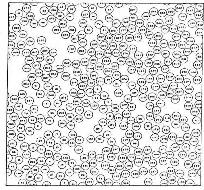
To identify the particles that are "effective" neighbors to some particle i) the locations in LMTX corresponding to the pattern of

sub-boxes shown in the diagram on the next page are examined and a

list of the non-zero entries compiled. The pattern is centered on the

sub-box occupied by particle_!, and special care must be taken with the LMTX indexing during the "search" to account for the periodic boundary conditions.

In later versions of the dynamics programming an alternative

method for neighbor identification was employed. It is assumed that no two particles further than 3. 5

a

apart can diffuse to within 2. 5

a

of

each other during an interval of 5 x 10-1 3 sec. The neighbor-search pattern was therefore extended to a radius of 3. 5 a, and lists of the

-

--

..

-...

.. 1o

/

'

_...

/ r-..

/

"

.

I \

I

"

I \

I \

~

I

I _I

\

I

\

_I

~

.

I

\ _/

"

_"

_... / 7

•

""

... _...

_.,.,,

,,,. . /

-

_--

-14-10- ...

Neighbor-search pattern for identifying the "effective" neighbors

to some particle

i.

in the system. The lighter lines show a

portion of the grid of 0. 5 a sub-boxes superimposed on the

space-box; particle

..!

lies in the crosshatched sub-box at the

center. All particles lying in the pattern of sub-boxes enclosed

by the heavy lines are assumed to be "effective" neighbors to

Between searches, the "effective" neighbors to any given particle

.!.

are

determined by examining the particles cited in its "extended" neighbor

list (taking account of the periodic boundary conditions, of course). If

at any time one of the neighbors is found to be more than 3. 5

a

from

.!. ,

its number is deleted from the list; thus the number of active entries

in the "extended" neighbor list for each particle decreases steadily

between searches.

This second technique for neighbor identification offers the

advantage that the system is searched for the neighbors to each particle

only periodically; a great deal of additional storage space is however

required by the programming to store the neighbor lists between

searches. Because of hardware (principally core storage) limitations

intrinsic to the IBM 7074 computer, the dynamics calculations were

f Ol .. md to proceed at about the same speed when either the fir st or second

neighbor identification techniques were employed. But if a computer

providing more core storage is used--and especially if a t

hree-dimensional model system is being simulated--the second technique

would appear to offer a more efficient means of keeping account of the

"effective" neighbors to each particle.

In addition to that required by the "neighbor search" operations,

the dynamics programming uses the following indexed storage:

DIMENSION PX(500), PY(500), X{500), Y{500),

VX{500), VY(500), AX(500), A Y(500),

TEMPX(500), TEMPY(500),

Let us assume that the program has just completed the cycle for time

r(n). Then PX(I) and PY(I) contain the x and y coordinates of particle

I for time r(n-1), X(I) and Y(I) the coordinates for time r(n), and

VX(I), VY(I) the velocity and AX(I), AY(I) the acceleration components

for time r(n). The calculation for cycle (n+l) proceeds as follows:

1. The predicted x and y coordinates of the particles at time

I

r(n+l} are computed according to eqn. (6). For each particle I:

PX(I)

=

PX(I) + 2(.6.T)

*

VX(I)

PY(I)

=

PY(I) + 2 (.6. T)

*

VY(I)

2. The predicted accelerations for time r(n+l} are computed

accord-ing to eqn~ (7). For each particle I, set TEMPX(I)

=

TEMPY(I)

=

0 and determine the list of "effective" neighbors to be included

in the summation. Then for each neighbor J to particle I,

cal-culate the distances

DX

=

PX(I) - PX{J)

DY = PY(I) - PY(J)

taking into account the periodic boundary conditions.

Calculate the powers of pij (n+l):

R2

=

DX**2 + DY**2

R6

=

R2 ** 3

R12

=

R6 ** 2

and the force factor:

Then sum the contributions of neighbor J into the component

accelerations of particle I:

TEMPX(I)

=

TEMPX(I) + DX* F

TEMPY(I) = TEMPY(I) +DY* F

3. The velocities for time r(n+l) are calculated according to eqn.

(8). For each particle I:

TEMPX(I)

=

VX(I) + !(.Ar)* (TEMPX(I) + AX(I))

TEMPY{I)

=

VY(!) + ~(Ar)* (TEMPY{I) + A Y(I))

are

4. The data -Hr rearranged, and positions for time r(n+l) calculated

according to eqn. (9). For each particle I:

PX{I)

=

X(I)

PY(!)

=

Y(I)

X(I)

=

PX(I) +!(Ar)* (TEMPX(I) + VX(I))

Y(I)

=

PY(I) + t(Ar) * (TEMPY{I) + VY(I))

and the velocity component values in VX(I) and VY(I) are

exchanged with those in TEMPX(I) and TEMPY(I), respectively.

Note: At this point, PX and PY contain the particle coordinates for

time r(n), TEMPX and TEMPY the velocity components for time r(n),

X and Y the new particle coordinates for time r(n+l), and VX and VY

the new velocity components for time r(n+l).

5. The component acceleration values for time r(n) are saved

AXN (I)

=

AX (I)

and new accelerations for time T(n+l) are computed using the same procedure as outlined under step 2 above--except that DX and DY are calculated from the coordinate values in the X and Y

vectors, and the acceleration components are summed into AX(I) and AY(I) instead of TEMPX(I) and TEMPY(I).

6. "Corrected" velocities and positions for time T(n+l) are computed according to eqns. (8) and (9), respectively. For each particle I:

VX(I)

=

TEMPX(I) + ~(AT)* (AX(I) + AXN(I)) VY(I) = TEMPY(I) + ~(AT)* (AY(I) +A YN(I))

X(I) = PX(I) + ~(AT)* (VX(I) + TEMPX(I))

Y(I)

=

PY(I) +~(AT)* (VY(I) + TEMPY(I))

7. "Corrected" accelerations are computed on the basis of the

"corrected" position values using the same procedure as outlined under step 2--except that DX and DY are calculated from the co

-ordinate values in the X and Y vectors, and the acceleration

components are summed into AX(I) and A Y(I) instead of TEMPX(I) and TEMPY(I).

Steps 6 and 7 may be repeated {iterated) as many times as desired.

The calculation then returns to step 1 for time T(n+2).

After each cycle in the dynamics integration, the positions and velocities of the particles are recorded on magnetic tape in a (4N

The first "tag0

word contains N in the decrement field and the "integer box dimension" (in units of 0. 5 a) in the address field;8 the second "tag" word contains the "true" space-box edge dimension (in units of a) in

floating-point format. Each cycle in the dynamics integration is assigned a "cycle number" (corresponding to the time-counter !!. used above) that is incremented after each step; this number is recorded in the third "tag" word. And finally, the data generated during a given

~c

execution of the dynamics program is assigned a six character alpha-meric data label. This label is recorded, in BCD format, in the fourth "tag" word.

D. · Auxilliary Procedures

The calculations for the model fluid were started with a system of 364 particles symmetrically arranged in four 91-particle hexagonal ncrystals" in a space-box with edge dimension 25. 0

a.

The particles in each crystal were placed in a perfect two-dimensional hexagonal closest-packed configuration with a lattice spacing of 21/6 a; the

crystals were centered in each of the four quadrants of the space-box.

To obtain a randomized thermal motion in the fluid, a value of 0. 33389 was randomly assigned, either positive or negative, to the x and y velocity components of each of the particles. Center-of-mass motion was then eliminated by, for example, summing the x-velocity

compo-nents, dividing the sum by 364, and subtracting the resulting "error component" from the x-velocity of each of the particles.

8

As shown by Fig. 1 in Paper No. 1 (page 58 ), the component velocities were found to achieve an equilibrium Gaussian distribution very quickly after the start of the dynamics calculations. The hexa-gonal closest-packed configuration with lattice spacing 21/6

a

(the potential minimum distance for the Lennard-Jones pair potential) was used so that the temperature of the fluid after equilibration could be predicted on the basis of the initial value assigned to the velocities. The symmetric disposition of particles within the space-box was required to prevent center-of-mass motion from being introduced through potential interactions between the particles. But because the system was found to achieve an equilibrium spatial configuration only rather slowly, the particles were initially arranged in a number of quick-melting "crystals" rather than a space-filling lattice.

Following the format developed in subsection C above, let us assume that the assigned particle coordinates for r(O) are stored in the X and Y vectors and the assigned velocity components in the VX and VY vectors. Component accelerations for r(O) can be computed from the assigned positions using the procedure described under step 2 in

the outline flow diagram, except that DX and DY are calculated from the coordinate values in the X and Y vectors and the acceleration co

n-tributions are summed into AX(I) and AY(I) instead of TEMPX and TEMPY. Then for the first cycle in the dynamics calculation, the pre-dicted positions for time r(l) are computed according to the formula:

x~ (1)

=

x-(O) + v.(O) (A:r) + ~ a.(O) (~r)2