Efficient Framework for Finding Optimal Data
Partitions for Hierarchical Centroid Algorithm
Romana Riyaz1, Irfan Rashid2 1, 2
Department of computer science University of Kashmir, Srinagar
Abstract:The most important task of clustering process is the validation of results obtained from clustering algorithms. There are many cluster validation criteria’s but the most commonly used approaches are founded on internal validity indices. There are numerous indices that have been suggested from time to time but there are only some of them that have been popularly used. In this paper we have drawn a comparative analysis of external and internal validity measures using clustering results from hierarchical-centroid algorithm; we show the results of our experimental work which can be useful in selecting the most suitable index and providing an insight about the performance of different indices on different datasets. We have used four datasets: Iris, Gene dataset, liver disorder and Seeds datasets from UCI repository in our experiment.
Keywords: cohesion; separation; validity indices; clustering algorithms; dissimilarity; mediod.
I. INTRODUCTION
Clustering is a process of partitioning a set of data (or objects) into a set of meaningful subclasses called clusters. Data clustering is a method of creating groups of objects or clusters in such a way that objects which are in one cluster are very similar than the objects in different clusters. Clustering is an important tool for a variety of applications in data mining and has received attention in many areas including engineering, medicine, biology and data mining. Hierarchical clustering method works by grouping data objects into a tree of clusters. Hierarchical clustering methods can be further classified as either agglomerative or divisive depending on whether the hierarchical decomposition is formed in a bottom up (merging) or top down (splitting) fashion. The quality of pure hierarchical clustering method suffers from its inability to perform adjustment once a merge or split has done. If a particular merge or split decision is a poor choice the method cannot backtrack and correct it. As such, merge points need to be chosen carefully. For improving the quality of cluster integration of hierarchical agglomeration with iterative relocation method is emphasized. All agglomerative hierarchical clustering algorithms begin with each object as a separate group. These groups are successively combined based on similarity until there is only one group remaining or a specified termination condition is satisfied. For n objects, n-1 merging is done. In this paper we have presented an extensive comparison of cluster validity indexes on various real datasets in order to search for an optimal number of clusters for Hierarchical-centroid algorithm. The next section discusses work related to cluster validity indices comparison, section III provides a brief description of Proposed iterative merging framework which is used for clustering data in our experiment, section IV describes the variouscluster validity indices (CVI’s) used in this paper and section V shows the experimental setup and section VI shows the main result work and finally we draw the conclusion and suggestion for further extensions.
II. RELATED WORK
There are internal validity indices based on the compactness within a cluster and the separation between clusters. The sum-of-squares based indices are founded on sum-of-sum-of-squares within cluster (SSW) and/or sum-of-sum-of-squares between clusters (SSB) values, for example, Ball and Hall [4], Hartigan[5], Calinski-Harabasz (CH) [6] and Xu[7]. WB-index [8] is a sum-of-squares based index where a minimum value can be attained as the number of clusters. Other popular indices are given in [8–12].Dunn-type indices [9] are based on the inter-cluster distance and diameter of a cluster hyper sphere. A Dunn index is sensitive to outliers, whereas the Davies and Bouldin index is defined by the average of cluster evaluation measures for all the clusters. S_Dbw [11] replaces the total separation with the density of data objects in the middle of two clusters and omits the weighting factor. A model selection method called the Bayesian information criterion (BIC) [12] has been used in model-based clustering, it can be adapted to partition-based clustering[13], too.
III. ITERATIVE MERGING FOR CLUSTERING DATA
We propose an iterative merging approach for obtaining optimal clusters of the given data set. Two clusters are merged during each iterative step until stopping criteria (described in next section) is satisfied. The iterative merging process is described in detail below.
Iterative merging approach is based on the concept of agglomerative (bottom-up) clustering method. The idea is to build optimal clusters, where data elements are separated by natural boundaries. Merging of two clusters is based on the concept of closeness. During each iterative step, two closest clusters are merged to create a new cluster. This process is continued until optimal clusters are obtained.
The closeness of two clusters can be computed by using centroid-linkage distance. centroid linkage clustering, distance ( , )between two clustersc1 and c2 centers is used. The average distance ( , ) is the distance between the centers of two cluster C1 and C2. Mathematically it can be written as:
D = || - ||
Here, where and are the centroids of cluster C1 and C2.
IV. STOPPING CRITERIA FOR MERGING
We propose using Cluster Validity Indices(CVI)as a stopping criteria for obtaining the optimal number of clusters for the given dataset. CVI’s determine how well each element is placed within its cluster. In general, clustering validity indices are defined by combining the measures of compactness and reparability. Compactness: This measure gives an indication of closeness of elements in a cluster. A common measure of compactness is given byintra cluster distance of elements in a cluster. Reparability: This measure gives an indication of how well a cluster is separated from other clusters. The intuitive way of expressing reparability is to compute inter cluster distances. On the type of the measure used (i.e. compactness measure reparability measure), we define three types of Cluster Validity Indices: i) Internal Cluster Validity Indices, this uses only compactness measure ii) External Cluster Validity Indices, this uses only reparability measure and iii) Hybrid Cluster Validity Indices, this uses both compactness and reparability measures.
A. Internal validity criteria
The internal validity indices quantify how good a particular partitioning is in terms of the compactness and separation between clusters and for this it utilizes the intrinsic structure of the data and does not require any supervised information. Some of internal validity indices are explained as under:
1) Silhouette index: Silhouete index refers to a method of interpretation and validation of clusters of data. The technique provides a succinct graphical representation of how well each object lies within its cluster by combining the measures of compactness and reparability. For each element i, leta ( ) be the average distance of i with all other elements within the same cluster. a( ) canbe interpreted as how well i is assigned to its cluster(the smaller the value, the better the assignment).Let b(i) be the lowest average distance of i to any other cluster of which i is not a member. The cluster with this lowest average distance is said to be the "neighboring cluster" of i because it is the next best fit cluster for point i. We now define:
Sil(i) = ( ) – ( ) ( ( ), ( ))
2) Calinski –Harabasz index: Calinski-Harabaszindexassess the quality of a clustering. It is given by the expression:
CH(k)= ( )( ) ( )( )
where k denotes the number of clusters and B(k) and W(k) denote the between (separation) and within (cohesion) cluster sums of squares of the partition, respectively. These are measured by the formula:
W=∑ ∑ ∈ ( − )2
B=∑ | | ( − )
where |Ci| is the size of cluster i. An optimal number of clusters is then defined as a value of k that maximizes CH(k).
3) Dunn index:The Dunn index is based on the identification of clusters which are well separated and compact and therefore to maximize the inter-cluster distance while minimizing the intra-cluster distance. For any partition U ↔A : ∪··· ∪··· , where represents the ith cluster of such partition, the Dunn‘s validation index, D, is given by equation:
DI (c) = ,
,
{∆( )}
, = , ,
∆( ) = ( , ) ,
Where d is a distance function, , is the inter-cluster distance and ∆( ) gives the maximum distance between the farthest two points within a cluster (diameter of cluster). Thus large values of D correspond to good clusters. Therefore, the number of clusters that maximizes D is taken as the optimal number of clusters.
4) Davies-bouldin index: Davies-Bouldin index was introduced by [10], it is an index which uses the measures of compactness and severability. Davies-Bouldin index (DB) is given by expression:
DB(k) = ∑ (∆ ∆ )
( , )
Where Δ( ) and Δ( ) denotes the intra-cluster distance, calculated as the average distance of all the cluster elements and to their respective cluster centers, whereas δ( , ) denotes the distance between the clusters and (distance between the cluster centers).Therefore, the optimum number of clusters corresponds to the minimum value of DB (k).
B. External validity criteria
External validity indices measure the quality of a clustering result by bringing in some kind of external information such as known class labels or some supervised information. External validation measures know ‘true’ number of clusters in advance. These indices mainly quantify how good is the obtained partitioning with respect to prior class labeled information available.
1) Rand index: Rand index is an absolute criterion or referential standard that allows the use of classification datasets for performance assessment, not only of classifiers (which can produce different data partitions with the right number of classes), but of clustering results (in which different data partitions can be composed of different numbers of clusters) as well. This index handles two hard partition R={ , … . , } as the actual partition(reference partition)of the dataset D and Q= { ,….., } as the clustering structure of the dataset D The reference partition, R, encodes the class labels, i.e., it partitions the data into k known classes. Partition Q,in turn partitions the data into s categories(classes or clusters), and is the one to be evaluated. The categories encoded by Q will be, from now on, called clusters. This way one can easily distinguish between them and right classes encoded by R.
Thus, Rand index is given as:
W=
Where:
c) Number of pairs of data objects belonging to different classes in R and to the same cluster in Q. d) Number of pairs of data objects belonging to different classes in R and to different clusters in Q.
Rand index can have following values: (i) W [0, 1]; (ii) = 0 iff Q is completely inconsistent, i.e., a = d = 0; and (iii) = 1 iff the partition under evaluation matches exactly the reference partition, i.e., b = c = 0 (Q = R).
2) Adjusted Rand index: Rand index is defined as the number of pairs of objects that are either in the same group or in different groups in both partitions divided by the total number of pairs of objects. The Rand index lies between 0 and 1. When two partitions agree perfectly, the Rand index achieves the maximum value 1.Now if we adjust rand index for the chance grouping of elements then that forms adjusted rand index.
3) Jaccard index: The jaccard index is used to evaluate the stability of a clustering method. The rationale behind this index is essentially same as that of Rand index, except for the absence of term‘d’. The term d is interpreted as a “neutral” term-counting pairs of objects that are not clearly indicative either of similarity or of inconsistency- in contrast to the others, viewed as counts of “good pairs”(term a) and “bad pairs”(terms b and c). From this viewpoint, the jaccard coefficient can be seen as a proportion of good pairs with respect to the sum of non-neutrals (good plus bad pairs).Given a pair of clustering solutions, R (reference partition) and Q (partition to be evaluated)for the same data set, the jaccard index between R and Q is then defined as:
J =
Where
a) Number of pairs of data objects belonging to the same class in R and to the same cluster in Q. b) Number of pairs of data objects belonging to the same class in R and to different clusters in Q. c) Number of pairs of data objects belonging to different classes in R and to the same cluster in Q.
The jacquard index ranges from 0 to 1, where a higher value indicates a higher similarity between cluster solutions.
4) Fowlkes-Mallows (FM) index: Fowlkes-Mallows index measures the similarity of resulting clusters with real partition of a dataset. Consider Q={ ,….., } as a clustering structure of a dataset D, and R={ , … . , } as the actual partition of the dataset. The state of each pair of elements pertains to one of the following four states:
a) Number of pairs of data objects belonging to the same class in R and to the same cluster in Q. b) Number of pairs of data objects belonging to the same class in R and to different clusters in Q. c) Number of pairs of data objects belonging to different classes in R and to the same cluster in Q.
Thus, Fowlkes–Mallows index, is defined as
FM= ( )(
)
A higher value for the Fowlkes–Mallows index indicates a greater similarity between the clusters and the benchmark classifications.
V. PROPOSED OPTIMAL CLUSTERING ALGORITHM
A. Step 1: Assign each data item to a cluster. N data items will result in N clusters where each cluster will have just one data item. Inter clusters distances between each pair of clusters is computed.
B. Step 2: Check for optimal number of clusters using indices. If optimal partition of data has been achieved then stop else proceed with step 3.
C. Step 3: Two closest clusters (determined using inter cluster distances) are merged into a single cluster. D. Step 4: Inter cluster distances are updated.
E. Step 5: Steps 2 and 3 are repeated until all items are clustered until stopping criteria is satisfied.
VI. EXPERIMENTAL SETUP
different values of ‘k’ and on different datasets respectively. Tables II-V shows the values obtained for each index for different datasets.
VII. RESULTS
Table IThe characteristics of the real datasets. Dataset No. of Objects Features Classes
Iris 150 4 3
Gene 72 39 3
Seed 210 7 3
Liver 345 7 2
A. Plots For Iris Dataset
C. Plots For Seed Dataset
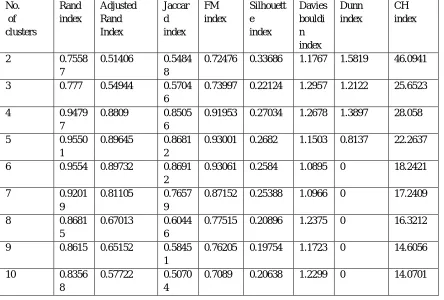
TABLE I Values for k obtained for iris database
TABLE II Values for k obtained for Gene database No. of clusters Rand index Adjusted Rand Index Jaccar d index FM index Silhouett e index Davies bouldin index Dunn index CH index
2 0.77629 0.56812 0.5951 4
0.77145 0.68639 0.3836 3.8212 501.9249
3 0.88591 0.7455 0.7118 6
0.83205 0.55508 0.5819 2.4132 554.9067
4 0.86228 0.68717 0.6522 0.78951 0.39645 0.67037 1.125 388.2909 5 0.83508 0.59963 0.5521
3
0.71967 0.34311 0.64608 1.2126 406.1216
6 0.81038 0.53003 0.4850 5
0.6671 0.32926 0.67791 1.4251 413.1072
7 0.81217 0.53376 0.4874 2
0.66986 0.31834 0.56939 1.4251 350.7682
8 0.80868 0.52061 0.4724 9
0.65969 0.29369 0.63393 1.4067 313.6823
9 0.80626 0.51355 0.4658 3
0.65425 0.28943 0.67366 1.4714 285.1101
10 0.80582 0.51224 0.4645
9
0.65324 0.27742 0.59895 0.0120 255.8146
No. of clusters Rand index Adjusted Rand Index Jaccar d index FM index Silhouett e index Davies bouldi n index Dunn index CH index
2 0.7558
7
0.51406 0.5484 8
0.72476 0.33686 1.1767 1.5819 46.0941
3 0.777 0.54944 0.5704 6
0.73997 0.22124 1.2957 1.2122 25.6523
4 0.9479
7
0.8809 0.8505 6
0.91953 0.27034 1.2678 1.3897 28.058
5 0.9550
1
0.89645 0.8681 2
0.93001 0.2682 1.1503 0.8137 22.2637
6 0.9554 0.89732 0.8691 2
0.93061 0.2584 1.0895 0 18.2421
7 0.9201
9
0.81105 0.7657 9
0.87152 0.25388 1.0966 0 17.2409
8 0.8681
5
0.67013 0.6044 6
0.77515 0.20896 1.2375 0 16.3212
9 0.8615 0.65152 0.5845 1
0.76205 0.19754 1.1723 0 14.6056
10 0.8356
8
0.57722 0.5070 4
[image:8.612.87.531.389.689.2]TABLE III Values for k obtained for Seed database
Table IV Values of K for Liver Disorder Dataset
No. of clusters Rand index Adjusted Rand Index Jaccard index FM index Silhouette index Davies bouldin index Dunn index CH index
2 0.72381 0.44782 0.50095 0.68201 0.47524 0.74269 2.2868 298.2568
3 0.76664 0.48391 0.49417 0.66205 0.42586 0.61777 2.3396 315.1461
4 0.7465 0.40696 0.4173 0.59035 0.3425 0.73483 1.608 266.5034
5 0.73092 0.3626 0.38148 0.55499 0.31504 0.73933 1.608 226.0421
6 0.75047 0.3847 0.37744 0.55887 0.29951 0.78018 1.6692 233.4473
7 0.77849 0.42253 0.37511 0.58349 0.32683 0.80426 1.4777 275.151
8 0.7753 0.4116 0.36448 0.57472 0.32578 0.79416 1.5102 252.0699
9 0.77366 0.4027 0.35342 0.56814 0.30785 0.81459 1.4369 237.026
10 0.76127 0.36112 0.31498 0.53372 0.31455 0.80761 1.4369 238.5425
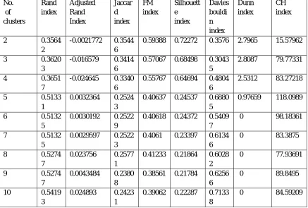
No. of clusters Rand index Adjusted Rand Index Jaccar d index FM index Silhouett e index Davies bouldi n index Dunn index CH index
2 0.3564
2
-0.0021772 0.3544 6
0.59388 0.72272 0.3576 2.7965 15.57962
3 0.3620
3
-0.016579 0.3414 6
0.57067 0.68498 0.3043 5
2.8087 79.77331
4 0.3651
7
-0.024645 0.3340 6
0.55767 0.64694 0.4804 6
2.5312 83.27218
5 0.5133
1
0.0032364 0.2524 3
0.40637 0.24537 0.6880 5
0.97659 118.0989
6 0.5132
5
0.0030192 0.2522 9
0.40618 0.24372 0.5409 7
0 98.18361
7 0.5132
5
0.0029597 0.2522 3
0.4061 0.23397 0.6134 6
0 83.3875
8 0.5274
7
0.023756 0.2577 1
0.41233 0.21864 0.6028 2
0 77.93691
9 0.5274
7
0.0043484 0.2380 8
0.38561 0.21784 0.6256 6
0 89.8495
10 0.5419
3
0.024893 0.2423 1
0.39062 0.22287 0.7133 8
[image:9.612.89.526.408.703.2]VIII. CONCLUSIONS
The main conclusions that we drew by the comparison of CVI’s is that external indicies outperformed internal indicies, however there are some of internal indices- Calinski-Harabasz index and duns index which gave good results on some of the datasets. However, the data does not show any conclusive observations to make any conclusion that some of the CVIs are significantly better
than the rest. Although external indices performed better but the major limitation of these indices is that they need external information which for real datasets is rarely available. So, we suggest the use of multiple indices for more reliable results. This work however raises some question which suggest for further extension which will be done in future papers.
REFERENCES
[1] Kaufman, L. and Rousseeuw, P.J. (1987), Clustering by means of Medoids, in Statistical Data Analysis Based on the L1–Norm and Related Methods, edited by Y. Dodge, North-Holland, 405–416.
[2] G. Milligan, M. Cooper, An examination of procedures for determining the number of clusters in a data set, Psychometrika 50 (1985) 159–179 [3] G. Ball, D. Hall, ISODATA, a novel method of data analysis and pattern classification, Menlo Park, Calif, Stanford Research Institute, 1965. [4] J. Hartigan, Clustering algorithms, John Wiley & Sons, Inc., New York, NY, USA, 1975.
[5] T. Calinski, J. Harabasz, A dendrite method for cluster analysis, Commun. Stat. 3 (1974) 1–27.
[6] L. Xu, Bayesian ying-yang machine, clustering and number of clusters, Pattern Recogn. Lett. 18 (1997) 1167–1178
[7] Q. Zhao, M. Xu, P. Fränti, Sum-of-square based cluster validity index and significance analysis, Proc. of the 17th Int. Conf. on Adaptive and Natural Computing Algorithms, 2009, pp. 313–322.
[8] J. Dunn, Well separated clusters and optimal fuzzy partitions, J. Cybern. 4 (1974) 95–104.
[9] D. Davies, D. Bouldin, Cluster separation measure, IEEE Trans. Pattern Anal. Mach. Intell. 1 (2) (1979) 95–104
[10] M. Halkidi, M. Vazirgiannis, Clustering validity assessment: finding the optimal partitioning of a data set, Proc. of the 2001 IEEE Int. Conf. on Data Mining (ICDM'01), 2001, pp. 187–194.
[11] S. Still, W. Bialek, How many clusters? An information theoretic perspective, Neural Comput. 16 (12) (2004) 2483–2506.
[12] D. Pelleg, A. Moore, X-means: extending K-means with efficient estimation of the number of clusters, Proc. of the 17th Int. Conf. on Machine Learning,2000, pp. 727–734
[13] R.C. Dubes, How many clusters are best? – an experiment, Pattern Recognition 20 (1987) 645–663.
[14] M. Brun, C. Sima, J. Hua, J. Lowey, B. Carroll, E. Suh, E.R. Dougherty, Model based evaluation of clustering validation measures, Pattern Recognition 40(2007) 807–82
[15] W. M. Rand (1971). "Objective criteria for the evaluation of clustering methods". Journal of the American Statistical Association (American Statistical Association) 66(336): 846- 850 JSTOR 2284239
[16] Peter J. Rousseeuw (1987). "Silhouettes: a Graphical Aid to the Interpretation and Validation of Cluster Analysis". Computational and Applied Mathematics 20: 53–65
[17] L.J. Hubert, J.R. Levin, A general statistical framework for assessing categorical clustering in free recall, Psychological Bulletin 83 (1976) 1072–1080. [18] S.C. Johnson,’’Hierarchical Clustering Schemes’’, Psychometrika 1967